Deep Image-Based Adaptive BRDF Measure

Wen Cao

Media and Information Technology, Department of Science and Technology, Link

oping University,

SE-601 74 Norrk

oping, Sweden

Keywords:

BRDF Measure, Adaptive, Deep Learning.

Abstract:

Efﬁcient and accurate measurement of the bi-directional reﬂectance distribution function (BRDF) plays a

key role in realistic image rendering. However, obtaining the reﬂectance properties of a material is both

time-consuming and challenging. This paper presents a novel iterative method for minimizing the number

of samples required for high quality BRDF capture using a gonio-reﬂectometer setup. The method is a two-

step approach, where the ﬁrst step takes an image of the physical material as input and uses a lightweight

neural network to estimate the parameters of an analytic BRDF model. The second step adaptive sample the

measurements using the estimated BRDF model and an image loss to maximize the BRDF representation

accuracy. This approach signiﬁcantly accelerates the measurement process while maintaining a high level of

accuracy and ﬁdelity in the BRDF representation.

1 INTRODUCTION

The bidirectional reﬂectance distribution function

(BRDF) (Nicodemus, 1965), is a fundamental con-

cept in computer graphics, representing the interac-

tion of light with a material. It is a four-dimensional

function that deﬁnes the relationship between incom-

ing and outgoing light directions at a material surface.

BRDFs can be represented either by analytic models

(Cook and Torrance, 1982; Phong, 1975) or by tab-

ulated measurements for every pair of incident and

outgoing angles (Matusik et al., 2003), with each ap-

proach having its own advantages and disadvantages.

The capture of real, physical BRDFs is an impor-

tant tool in many applications ranging from photo-

realistic image synthesis and predictive appearance

visualization —such as in additive manufacturing—to

enabling accurate sensor simulation and modeling of

scattering behaviors in industrial processes. However,

detailed BRDF measurement is a time-consuming

process because it typically requires dense mechan-

ical scanning of light sources and sensors across the

entire hemisphere. Several studies (Liu et al., 2023;

Dupuy and Jakob, 2018) have been conducted to re-

duce capture time by taking fewer measurements. Re-

cently, neural approaches (Zhang et al., 2021; Gao

et al., 2019) have been proposed to represent synthetic

BRDFs from images, primarily by estimating the an-

https://orcid.org/0000-0002-2507-7288

alytic BRDF parameters.

The objective of this paper is to accelerate BRDF

measurements using gonio-reﬂectometer setups, see

e.g. (Nielsen et al., 2015; Foo et al., 1997). To in-

corporate prior knowledge of the measured material,

our method uses a small neural network that takes an

image of the material as input to estimate the conﬁg-

uration of a small set of sampling directions to enable

efﬁcient BRDF measurement. Speciﬁcally, we em-

ploy an encoder network to estimate the reﬂectance

parameters of analytic BRDF models from the input

image, which are used to adapt the BRDF measure-

ment directions. The method leverages both analytic

BRDF models and image-based neural decomposition

as priors. These two priors are essential for efﬁciently

utilizing small networks to estimate the adaptive sam-

ple distribution.

In summary, we present a novel solution for

BRDF measurement with the following key contribu-

tions:

• Lightweight. Our approach utilizes images

to learn priors, eliminating the need for com-

plex measurement procedures. This signiﬁcantly

streamlines the measurement process and estab-

lishes an end-to-end pipeline.

• Adaptive and Accuracy. Experimental re-

sults demonstrate that our image-based adaptive

method effectively measure a wide range of ma-

terials. Its adaptability leads to highly accurate

292

Cao, W.

Deep Image-Based Adaptive BRDF Measure.

DOI: 10.5220/0013201000003912

Paper published under CC license (CC BY-NC-ND 4.0)

In Proceedings of the 20th International Joint Conference on Computer Vision, Imaging and Computer Graphics Theor y and Applications (VISIGRAPP 2025) - Volume 1: GRAPP, HUCAPP

and IVAPP, pages 292-299

ISBN: 978-989-758-728-3; ISSN: 2184-4321

rendered results for each material,outperforming

previous methods at some aspects.

2 RELATED WORK

In this section, we review previous work related to

BRDF measurement and neural spatially varying bidi-

rectional reﬂectance distribution function-SVBRDF

capture.

BRDF Measurement: is commonly done using go-

nioreﬂectometers, which capture the reﬂectance of

realistic materials by controlling mechanical light

sources and camera motions (Foo et al., 1997).

For example, acquiring the MERL dataset re-

quires totaling approximately 1.46 million sam-

ples (Rusinkiewicz, 1998; Matusik et al., 2003). To

accelerate the acquisition, several methods and de-

vices have been developed. Nielsen et al. (Nielsen

et al., 2015) and Miandji et al. (Miandji et al., 2024)

used the measured BRDF Dataset to train a basis to

linearly reconstruct the full BRDF samples to accel-

erate the measurements. Dupuy et al. (Dupuy and

Jakob, 2018) used a laser machine to measure the

NDF values of materials to adaptive sample the hemi-

sphere domain. Liu et al. (Liu et al., 2023) used a

meta-learning method to optimize the sampling count

of different BRDF models.

Neural (SV)BRDF Capture. Researchers are

exploring deep learning methods to develop

lightweight approaches for measuring (SV)BRDF

values (Kavoosighaﬁ et al., 2024; Gao et al., 2019).

Deschaintre (Deschaintre et al., 2019) used an

encoder-decoder network to estimate the normal,

diffuse albedo, and roughness images from phone-

captured images. Zhang (Zhang et al., 2021) used

images as input to predict BRDF values for each

pixel based on NeRF output. Zeng (Zeng et al., 2024)

used a diffusion framework to decompose RGB

images into normal, albedo, roughness, metallicity

and diffuse maps.

3 APPROACH

Our method employs a Convolutional Neural Net-

work (CNN) encoder to estimate the BRDF param-

eters of an analytic model from a single image. Based

on the estimated BRDF model, we utilize importance

sampling to derive an adaptive sampling pattern for

the input material. These sampling values are used to

render the estimated image by bilinear interpolation.

The renderd images with measured samples are fed

back to the sample selector, which calculates the im-

age loss and determines the optimal number of sam-

ples for the next iteration as illustrated in Figure 1.

3.1 BRDF Estimation

Drawing inspiration from deep learning techniques

used in SVBRDF capture (Deschaintre et al., 2019)

from images, we train a convolutional neural network

to encode isotropic material images into their corre-

sponding appearance parameters for a set of analyti-

cal models. The architecture of the BRDF estimation

network is illustrated in Figure 2 and employs sig-

moid activation functions for the parameter outputs.

3.1.1 Analytic BRDF

We use the Ward BRDF model (Walter, 2005)

parameterized by its diffuse reﬂection coefﬁcient

,roughness α and specular reﬂection coefﬁcient ρ

to train the network. The isotropic Ward BRDF

(i, o) with incoming direction i and outgoing di-

rectin o is:

(i, o) =

4πα

√

cosθ

−

tan

(1)

where θ

,θ

is the incoming angle, outgoing angle,

half angle.

To train the encoder network, we use the Loss

function of Ward BRDF model as below

loss

= ∥

I −I∥

+ ∥(

α) −(ρ

, α)∥

(2)

where I represents the rendered image based on the

BRDF parameters. L1 loss is used for both images

and parameters.

3.1.2 Measured BRDF

We use the Measured BRDFs Dataset (MERL) (Ma-

tusik et al., 2003) for training and validation. We pre-

dict roughness, α, for each image by training from the

neural BRDF network from scratch.

(i, o) = f

′

ggx

(α) (3)

where f

′

ggx

is the microfacet BRDF model (Zhang

et al., 2021)representing the reﬂectance. We optimize

the network to minimize the loss between estimation

and ground truth of alpha value and images.

loss

= ∥

I −I∥

+ ∥(

α) −(α) ∥

(4)

The ground truth alpha values for each MERL

material are derived by ﬁtting their respective total

BRDF data to the microfacet BRDF model. Based

on the BRDF parameters estimated by the network,

Deep Image-Based Adaptive BRDF Measure

293

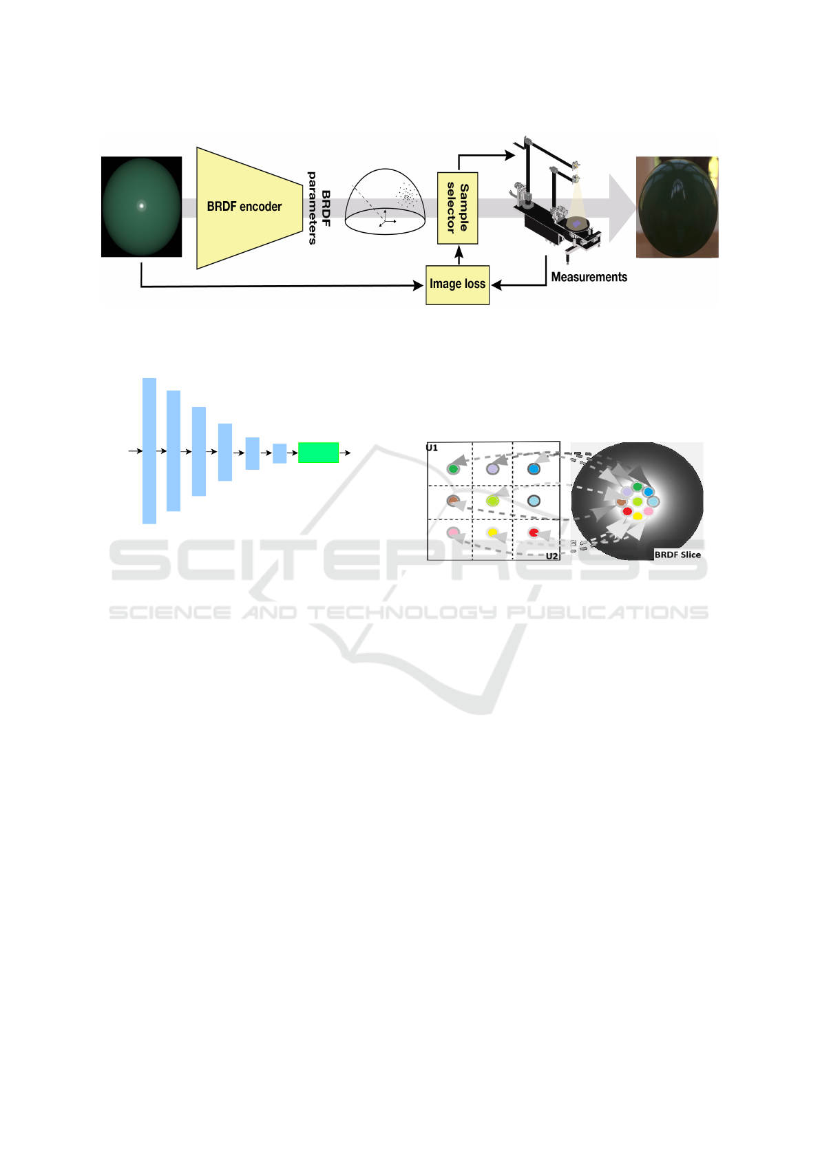
Figure 1: Method Flowchart of Deep Image-based Adaptive Reﬂectance Measure. For a ﬁxed material, we use its image as

input to an encoder network, which then estimates the BRDF parameters for it. An adaptive sampler use these parameters to

determine the outgoing direction locations. Finally, we progressively increase the number of these locations to achieve the

minimum number of samples required while maintaining high ﬁdelity.

256

Image

Input

128

BRDF

Parameters

Figure 2: Illustration of the encoder network architecture

used for estimating BRDF parameters. Blue boxes denote

convolutional layers with batch normalization and ReLU

activation functions. The dimensions of these layers are the

numbers inside them. The green box represents a fully con-

nected layer outputting the BRDF parameters.

the estimated images

I are rendered using the Micro-

facet BRDF model. We employed an L1 loss between

the predicted images

I and the ground truth images

I,while an L2 loss was applied to the parameter esti-

mations.

3.2 Adaptive Reﬂectance Sampling

Using the BRDF estimation network, we are able to

derive the BRDF parameters from an input image. We

draw inspiration from previous work and utilize the

inverted BRDF importance sampling to drive an adap-

tive sampling distribution of the outgoing hemisphere

which is similar to the work of Dupuy et al. (Dupuy

and Jakob, 2018; Bai et al., 2023). This adaptive

sampling strategy effectively minimizes measurement

time by targeting only those directions speciﬁed by

the input BRDF material pattern. For instance, in

the case of a mirror-like material, sampling is con-

centrated on the delta regions directly opposite the in-

coming light direction. In contrast, for diffuse ma-

terials, a uniform sampling pattern is implemented

throughout the hemisphere. In practice, the BRDF

sampling pattern for most materials typically falls be-

tween these two extremes. For details on importance

sampling, we refer to Bai et al. (Bai et al., 2023).

Figure 3: A visualization of the process g in Eq. 5 to cal-

culate the adaptive sampler’s position. We start by get-

ting sample points (u

, u

) on a uniform grid in the unit

square [0, 1]

. The importance sampling process takes a

sample point (u

, u

), and maps it to position on a 2D BRDF

slice,and reverse wise works by its inverse function.

The rendering equation of general BRDF model is

as follows:

I(i) =

(i, g(u)) L

(g(u))

∥

(u)

∥

du (5)

where L

is the incident radiance, I

denotes the radi-

ance reﬂected in all directions at pixel point i, J

is the

Jacobian of g.

p(ω

) = w

·p

(ω

) + w

·p

(ω

)

(6)

where w

+ w

= 1, p(ω

) is the PDF of outgoing di-

rection ω

. The diffuse PDF p

is a simple cosine-

weighted distribution and PDF p

is the specular dis-

tribution based on BRDF specular lobe.The equation

g deﬁnes the adaptive sampling strategy in the out-

going hemisphere domain according to the specular

distribution p

without the diffuse distribution as Fig-

ure 3 and its inverse g

−1

map the location of BRDF

slice back to the unit square which is used in bilinear

interpolation to fully evaluate the BRDF values in the

rendering function to produce the image.

GRAPP 2025 - 20th International Conference on Computer Graphics Theory and Applications

294

Thus, we focus on samplers suitable for represent-

ing f

: an invertible function g from random variates

u ∈ [0, 1]

into outgoing directions ω

and its asso-

ciated probability density function (PDF) p(ω

, ω

The shape of p should closely matches f

to achieve

low variance.

3.2.1 Importance Sampling

The importance sampling equation for the Ward

BRDF model used in this work is:

= arctan(α

−log u

)

= 2πu

(7)

where φ

, θ

is the half angle; u

, u

is the uniform

variates on [0, 1]

(Walter, 2005). We compute the

inverse of Equation 7 to evaluate the measured BRDF

parameters in the rendering equation using:

= e

−

tan

2π

(8)

Then, we use ω

= 2(ω

·ω

)ω

−ω

to determines

the outgoing direction ω

(φ

, θ

For the MERL dataset, there is no analytical

function for obtaining the PDF. Therefore, we ap-

proximate the PDF using the microfacet BRDF

model (Dupuy, 2015) and employ its importance sam-

pling method to achieve adaptive measurements. Ad-

ditionally, we utilize the inverse of this function in the

rendering process. Detailed functions and methodolo-

gies can be found in Dupuy’s Ph.D. thesis (Dupuy,

2015)

Based on the importance sampling procedures ex-

plained above, we adaptively sample the outgoing di-

rection according to the PDF and subsequently use

the direction to make a new measurement of the ma-

terial BRDF. Thus, previous measurements guide the

goniometer and facilitate precise and efﬁcient mea-

surement of the input material with reduced capture

time. The incoming directions are uniformly sampled

within the cosine-weighted hemisphere.

4 IMPLEMENTATION

We use Mitsuba 3.0 (Jakob et al., 2022) and its Python

bindings to render images of size 256 ×256 and Py-

Torch to implement the neural network.

4.1 Dataset

To train the neural network of the Ward BRDF model,

we create a dataset covering the full range of Ward

BRDF parameter-α.Images with varying roughness

and diffuse values were rendered using the Ward

BRDF function, a single point light source, and a

sphere in Mitsuba. The dataset consists of 4,000 train-

ing images and 100 test images.

Similarly, for the MERL dataset, we ﬁt each ma-

terial to the Microfacet BRDF model. We ﬁrst cre-

ate datasets by rendering images with varying alpha

and albedo values using the Microfacet BRDF model.

These images are used to pretrain the BRDF estima-

tion network, addressing the limited amount of mea-

sured data in the MERL dataset. We then ﬁne-tune the

BRDF estimation network using the MERL training

images, with the ﬁtted alpha values serving as ground

truth. The Microfacet dataset comprises 40,000 train-

ing images and 100 test images, while the MERL

dataset includes 85 training images and 15 test images

rendered with different materials.

4.2 Estimation

The BRDF estimation network are depicted in Fig-

ure 2 . We train the network in Nivida Geforce RTX

4080 with 15GB memory.

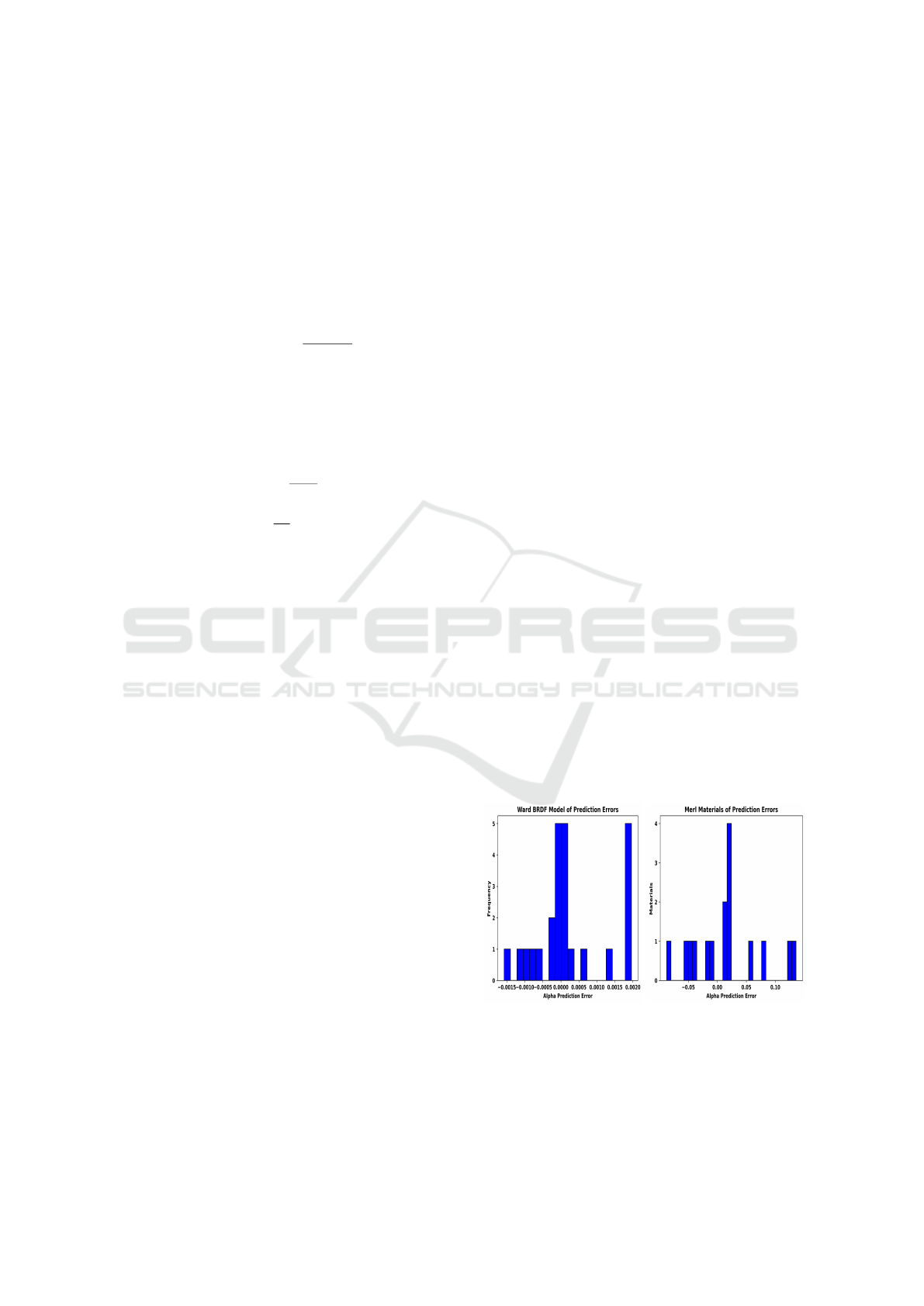
We demonstrate that our BRDF estimation net-

work accurately predicts BRDF parameters for both

the Ward model and the MERL dataset, as illustrated

in Figure 4. For the Ward BRDF model, the net-

work achieves nearly perfect predictions with errors

between -0.0015 and 0.0020. For the 15 materials

in the MERL test set, the estimation errors range be-

tween –0.1 and 0.1. In most BRDF models, albedo

represents the base color, while alpha describes the

shape of the BRDF reﬂection lobe. Since the base

color is visually evident in our results, we primarily

present the network’s alpha estimations in Figure 4.

Figure 4: Error distributions for BRDF parameters estima-

tion. It can be seen that the error varies in a small range.

Deep Image-Based Adaptive BRDF Measure

295

4.3 Sample Count

We treat the number of outgoing directions as hyper-

parameters of the entire pipeline. For each material,

we optimize the number of samples by the image loss

between the rendered images by the measurements

and the ground truth.

However we observe that the performance plots

based on sample number vary across different materi-

als, as shown in Figure 5. Generally, materials with

higher specular reﬂections require more samples. To

minimize the size of the measurements, we set the

maximum direction count to 32 ×32, as increasing

the number of samples beyond this point yields visu-

ally negligible improvements for most materials.

For the number of incident directions, we use one

φ point and eight θ points sampled from a uniform

cosine distribution, adhering to the rotational sym-

metry of isotropic materials. The number of direc-

tions was determined based on the work by Dupuy

and Jakob (Dupuy and Jakob, 2018).

5 RESULTS

In this section, we present the qualitative results and

comparisons with state-of-the-art methods for BRDF

acquisition. For quantitative evaluations, we em-

ploy metrics as Peak Signal-to-Noise Ratio (PSNR),

Root Mean Square Error (RMSE), and mean

LIP

error (Andersson et al., 2020). Additionally, we use

LIP error maps to visualize the errors in the rendered

images.

5.1 Comparison

Here, we compare our method with the state of the

art method meta-learning brdf sampling method (Liu

et al., 2023). Since Liu’s method learns sample pat-

terns for all materials, its performance does not im-

prove with increased sample counts once highlights

are achieved. Additionally, it requires the implemen-

tation of a ﬁxed sample count. In contrast, we derive

adaptive sampling pattern for each speciﬁc input ma-

terial, allowing the performance to progressively in-

crease as more samples are added.

We show the comparison between our method and

Liu’s method in Table 1, using the nine test materials

from our test datasets derived from the MERL dataset.

For quantitative comparison, we select results from

Liu’s method and our results with same sample num-

bers.

Speciﬁcally, Liu’s method uses from 32 to

512 samples within the Rusinkiewicz parameteriza-

tion (Rusinkiewicz, 1998), while our approach adopts

a conﬁguration of 1 ×8 incoming directions(θ

, φ

)

and from 2×2 to 8 ×8 outgoing directions(θ

out

, φ

out

)

in spherical coordinates.

Our method consistently produces high-ﬁdelity

rendered images across all tests, particularly with an

relative high number of samples. In contrast, Liu’s

method performs well with fewer samples, but its ac-

curacy declines as the sample count grows. For dif-

fuse and specular materials, our approach performs

comparable with Liu’s, as demonstrated by the results

in Table 1.

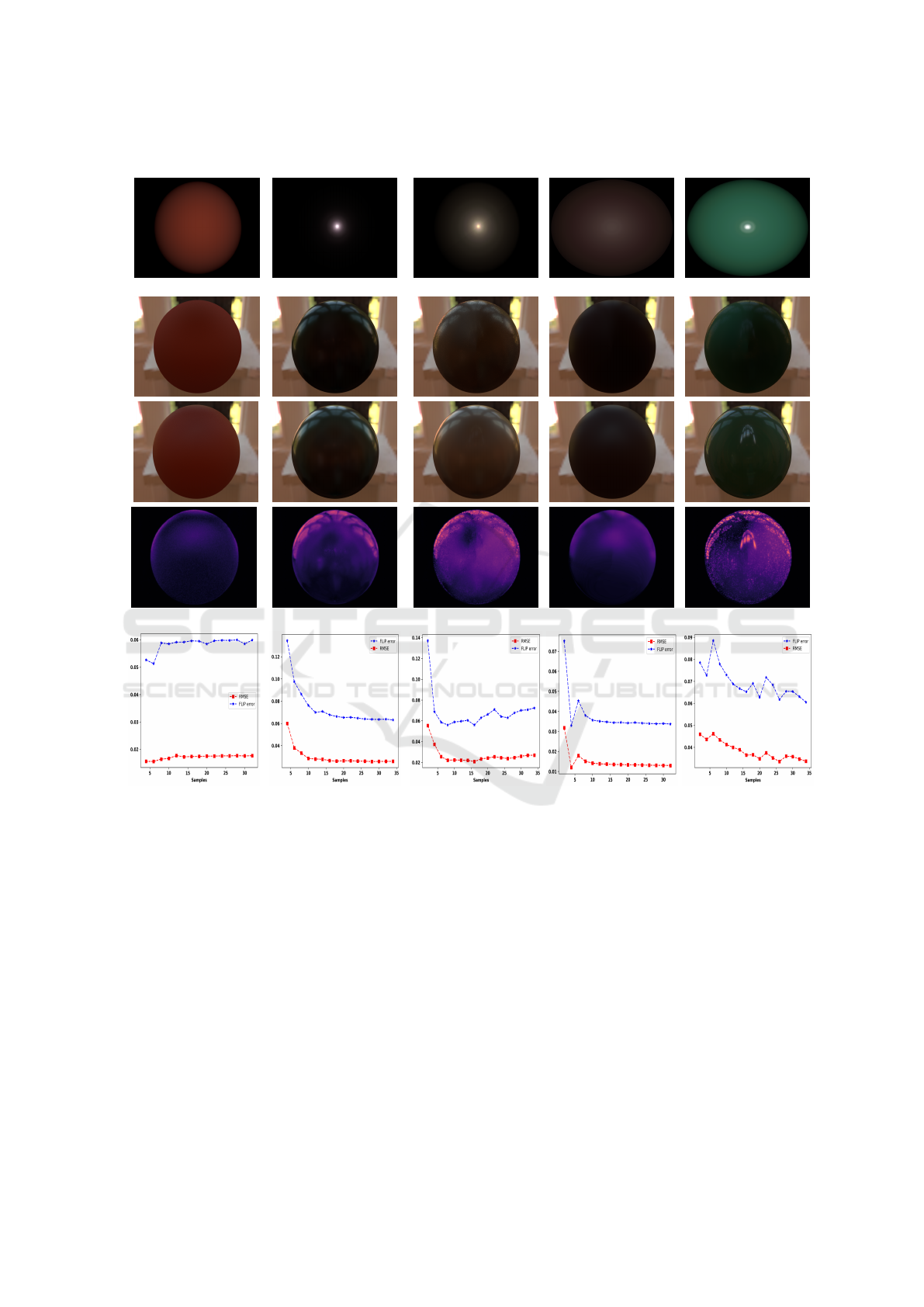
5.2 Evaluation on Different Materials

We show more visual results in Figure 5 with ﬁve

different materials. We observe that diffuse materi-

als achieve high-quality results with fewer samples,

whereas highly specular materials require a larger

number of samples to produce good outcomes. The

ﬁrst row and second row are the rendered images us-

ing our adaptive measurement method under point

lighting and environment lighting, respectively. The

fourth rows of Figure 5 shows the

LIP Error im-

age comparing the second row (rendered images from

our method) with the third row (ground truth), where

specular materials generally exhibit higher errors.The

last row presents the plot of the performance metrics

based on sample numbers, illustrating how the sam-

ple count is selected for each material as described in

subsection 4.3.

6 DISCUSSION

Moreover, additional variants in sample methods and

BSDF models could be further explored within this

approach.

Sample Method. Normalizing Flows (M

uller et al.,

2019) is a possible alternative to our adaptive sam-

pler, as it supports both inverse and forward sampling

and can be co-optimized with the entire pipeline. In-

vestigating the integration of Normalizing Flows into

our sampling strategy could be a valuable direction

for future research, offering potential improvements

in efﬁciency and versatility.

BSDF Model. We evaluated both the Ward BRDF

model and the Microfacet BRDF model, and our ﬁnd-

ings indicate that both models perform effectively

within our method. However, our current work is lim-

ited to isotropic materials.

In future research, we aim to extend our approach

to incorporate more complex BSDF models, such as

layered BRDFs, subsurface scattering materials, and

GRAPP 2025 - 20th International Conference on Computer Graphics Theory and Applications

296

Table 1: Comparing, Liu’s method (Liu et al., 2023),and our Adaptive sampler using all test Materials. The proposed

method is in blue and best values are in bold. Note samples of Liu’s method is in Rusinkiewicz parameterization((φ

, θ

))

(Rusinkiewicz, 1998), while our sample’s location is in spherical coordinates((θ

, φ

, θ

out

, φ

out

)).

Test Method Liu (Liu et al., 2023) Method

Image-

based

Adaptive

Materials Samples Count RMSE PSNR Samples Number RMSE PSNR

Alum-bronze 32 0.00154 36.26 1 ×8 ×2 ×2 0.055 25.1

128 0.00142 36.97 1 ×8 ×4 ×4 0.037 28.53

512 0.016 35.86 1 ×8 ×8 ×8 0.02 33.84

Dark-red-paint 32 0.0167 35.44 1 ×8 ×2 ×2 0.026 31.8

128 0.0239 32.43 1 ×8 ×4 ×4 0.0156 36.13

512 0.026 31.68 1 ×8 ×8 ×8 0.016 35.68

Color-changing-paint3 32 0.044 27.23 1 ×8 ×2 ×2 0.049 26.18

128 0.0335 29.5 1 ×8 ×4 ×4 0.06 24.43

512 0.0249 32.1 1 ×8 ×8 ×8 0.033 29.54

Dark-specular-fabric 32 0.026 31.56 1 ×8 ×2 ×2 0.032 29.95

128 0.034 29.44 1 ×8 ×4 ×4 0.012 38.43

512 0.033 29.7 1 ×8 ×8 ×8 0.015 36.45

Green-acrylic 32 0.03 30.5 1 ×8 ×2 ×2 0.046 26.76

128 0.07 23.1 1 ×8 ×4 ×4 0.044 27.21

512 0.05 26 1×8 ×8 ×8 0.043 27.26

Pink-fabric 32 0.02 33.94 1 ×8 ×2 ×2 0.04 27.853

128 0.02 33.92 1 ×8 ×4 ×4 0.025 32.16

512 0.026 31.53 1 ×8 ×8 ×8 0.0234 32.62

Red-fabric2 32 0.025 32.1 1 ×8 ×2 ×2 0.024 32.49

128 0.032 30 1×8 ×4 ×4 0.01 39.72

512 0.035 29.2 1 ×8 ×8 ×8 0.0098 40.17

Green-metallic-paint 32 0.067 23.42 1 ×8 ×2 ×2 0.056 25

128 0.028 31.13 1 ×8 ×4 ×4 0.0246 32.17

512 0.0271 31.32 1 ×8 ×8 ×8 0.02 33.94

White-diffuse-bball 32 0.04 28.47 1 ×8 ×2 ×2 0.0221 30.36

128 0.038 28.3 1 ×8 ×4 ×4 0.031 30.22

512 0.022 32.98 1 ×8 ×8 ×8 0.029 30.65

Specular-orange-phenolic 32 0.039 28.2 1 ×8 ×2 ×2 0.077 22.3

128 0.062 24.1 1 ×8 ×4 ×4 0.053 25.57

512 0.0462 26.71 1 ×8 ×8 ×8 0.0345 29.2

Red-metallic-paint 32 0.04 28 1×8 ×2 ×2 0.081 21.86

128 0.05 26.2 1 ×8 ×4 ×4 0.058 24.7

512 0.04 27.5 1 ×8 ×8 ×8 0.0294 30.6

Pink-plastic 32 0.013 37.92 1 ×8 ×2 ×2 0.078 23.25

128 0.02 33.99 1 ×8 ×4 ×4 0.048 26.42

512 0.019 34.58 1 ×8 ×8 ×8 0.019 34.56

PVC 32 0.038 28.44 1 ×8 ×2 ×2 0.064 23.83

128 0.03 30 1×8 ×4 ×4 0.046 26.71

512 0.031 30.2 1 ×8 ×8 ×8 0.023 32.8

Light-red-paint 32 0.018 34.85 1 ×8 ×2 ×2 0.082 21.76

128 0.029 30.82 1 ×8 ×4 ×4 0.042 27.52

512 0.0283 31 1 ×8 ×8 ×8 0.025 31.94

Maroon-plastic 32 0.033 29.65 1 ×8 ×2 ×2 0.068 23.25

128 0.063 24.1 1 ×8 ×4 ×4 0.054 25.3

512 0.04 27.4 1 ×8 ×8 ×8 0.03 30.4

Deep Image-Based Adaptive BRDF Measure

297

Dark-red-paint Color-changing-paint3 Alum-bronze Dark-specular-fabric Green-acrylic

Single Point LightEnvironment Light

Ground Truth

LIP Error

8 ×8 16 ×16 16 ×16 14 ×14 32 ×32

Performance Plot

Figure 5: Rendered sphere of Five Different Materials from the MERL Dataset.The ﬁrst row shows our measurements ren-

dered under single-point lighting. The second row shows our measurements rendered under environmental lighting. The third

row shows the ground truth rendered under the same environmental lighting conditions. The fourth row shows the

LIP error

images between the second and third rows. The ﬁnal row presents a plot of error metric values versus the number of samples

for each material. The Y-axis of ﬁnal row represents the RMSE and

LIP error values, while the X-axis indicates the sample

counts, ranging from 2 ×2 to 32 ×32 of outgoing directions.

anisotropic materials. We believe the adaptive capa-

bilities of our method could be further leveraged to

handle these complicated material representations ef-

fectively.

7 CONCLUSION

We propose an image-based adaptive BRDF sam-

pling method that signiﬁcantly reduces BRDF mea-

surement time while maintaining high accuracy and

ﬁdelity. We use a lightweight neural network and

show that it can accurately estimate BRDF parameters

and that this, in turn, can be used to importance sam-

pling new directions for taking measurements. We

validate our approach using both the MERL dataset

and the Ward BRDF model. Additionally, we com-

pare our method against the state-of-the-art method

by Liu et al (Liu et al., 2023).

Our method demonstrates some improved perfor-

mance in some aspects. By adaptively sampling each

material independently, without relying on references

from other materials, our technique ensures that addi-

GRAPP 2025 - 20th International Conference on Computer Graphics Theory and Applications

298

tional measured samples directly contribute to a more

accurate BRDF representation. This characteristic

distinguishes our method from previous approaches

and results in a more robust representation. Conse-

quently, our approach exhibits enhanced reliability.

ACKNOWLEDGEMENTS

This project has received funding from the European

Union’s Hori- zon 2020 research and innovation pro-

gram under Marie Skłodowska- Curie grant agree-

ment No956585. We thank the anonymous reviewers

for their feedback.

REFERENCES

Andersson, P., Nilsson, J., Akenine-M

oller, T., Oskarsson,

M.,

Astr

om, K., and Fairchild, M. D. (2020).

LIP:

A Difference Evaluator for Alternating Images. Pro-

ceedings of the ACM on Computer Graphics and In-

teractive Techniques, 3(2):15:1–15:23.

Bai, Y., Wu, S., Zeng, Z., Wang, B., and Yan, L.-Q. (2023).

Bsdf importance baking: A lightweight neural solu-

tion to importance sampling general parametric bsdfs.

Cook, R. L. and Torrance, K. E. (1982). A reﬂectance model

for computer graphics. ACM Transactions on Graph-

ics (ToG), 1(1):7–24.

Deschaintre, V., Aittala, M., Durand, F., Drettakis, G., and

Bousseau, A. (2019). Flexible svbrdf capture with a

multi-image deep network.

Dupuy, J. (2015). Photorealistic Surface Rendering with

Microfacet Theory. PhD thesis.

Dupuy, J. and Jakob, W. (2018). An adaptive parameteri-

zation for efﬁcient material acquisition and rendering.

ACM Transactions on Graphics, 37(6):1–14.

Foo, S. C. et al. (1997). A gonioreﬂectometer for measur-

ing the bidirectional reﬂectance of material for use in

illumination computation. PhD thesis, Citeseer.

Gao, D., Li, X., Dong, Y., Peers, P., Xu, K., and Tong,

X. (2019). Deep inverse rendering for high-resolution

SVBRDF estimation from an arbitrary number of im-

ages. ACM Transactions on Graphics, 38(4):1–15.

Jakob, W., Speierer, S., Roussel, N., Nimier-David, M.,

Vicini, D., Zeltner, T., Nicolet, B., Crespo, M.,

Leroy, V., and Zhang, Z. (2022). Mitsuba 3 renderer.

https://mitsuba-renderer.org.

Kavoosighaﬁ, B., Hajisharif, S., Miandji, E., Baravdish, G.,

Cao, W., and Unger, J. (2024). Deep svbrdf acqui-

sition and modelling: A survey. Computer Graphics

Forum, 43.

Liu, C., Fischer, M., and Ritschel, T. (2023). Learning to

learn and sample brdfs. Computer Graphics Forum

(Proceedings of Eurographics), 42(2):201–211.

Matusik, W., Pﬁster, H., Brand, M., and McMillan, L.

(2003). A data-driven reﬂectance model. ACM Trans.

Graph., 22(3):759–769.

Miandji, E., Tongbuasirilai, T., Hajisharif, S., Kavoosighaﬁ,

B., and Unger, J. (2024). Frost-brdf: A fast and robust

optimal sampling technique for brdf acquisition. IEEE

transactions on visualization and computer graphics,

PP.

uller, T., Mcwilliams, B., Rousselle, F., Gross, M., and

Nov

ak, J. (2019). Neural Importance Sampling. ACM

Transactions on Graphics, 38(5):1–19.

Nicodemus, F. E. (1965). Directional reﬂectance and emis-

sivity of an opaque surface. Applied optics, 4(7):767–

775.

Nielsen, J. B., Jensen, H. W., and Ramamoorthi, R. (2015).

On optimal, minimal BRDF sampling for reﬂectance

acquisition. ACM Transactions on Graphics, 34(6):1–

11.

Phong, B. T. (1975). Illumination for computer generated

pictures. Commun. ACM, 18(6):311–317.

Rusinkiewicz, S. M. (1998). A new change of variables

for efﬁcient brdf representation. In Rendering Tech-

niques’ 98: Proceedings of the Eurographics Work-

shop in Vienna, Austria, June 29—July 1, 1998 9,

pages 11–22. Springer.

Walter, B. (2005). Notes on the ward brdf.

https://www.graphics.cornell.edu/ bjw/wardnotes.pdf.

Zeng, Z., Deschaintre, V., Georgiev, I., Hold-Geoffroy,

Y., Hu, Y., Luan, F., Yan, L.-Q., and Ha

san, M.

(2024). Rgb↔x: Image decomposition and synthesis

using material- and lighting-aware diffusion models.

In ACM SIGGRAPH 2024 Conference Papers, SIG-

GRAPH ’24, New York, NY, USA. Association for

Computing Machinery.

Zhang, X., Srinivasan, P. P., Deng, B., Debevec, P., Free-

man, W. T., and Barron, J. T. (2021). NeRFactor: neu-

ral factorization of shape and reﬂectance under an un-

known illumination. ACM Transactions on Graphics,

40(6):1–18.

Deep Image-Based Adaptive BRDF Measure

299