Introducing the Cluster-Momentum Portfolio in Alternative Risk

Premia Investing

Berouz Fatemi

, Alireza Kobravi

, Duncan Larraz

, Francesc Naya

and Nils S. Tuchschmid

Investcorp-Tages, 39 St James’s Street, SW1A 1JD London, U.K.

Haute Ecole de Gestion de Fribourg, HES-SO, University of Applied Sciences and Arts Western Switzerland, Chemin du

Musée 4, CH-1700, Fribourg, Switzerland

Keywords: Alternative Risk Premia, Unsupervised Clustering, Portfolio Management, Alternative Investments.

Abstract: Managing alternative risk premia (ARP) portfolios is a challenging task, due to the complexities of these types

of investments. In this article, we present a purely quantitative approach that relies on performance persistence

among ARP strategies while ensuring diversification by classifying the ARP indices using unsupervised

hierarchical clustering. This cluster-momentum portfolio shows a superior performance when compared to a

set of internally built benchmarks and also of existing ARP asset manager funds. It seems that persistence in

performance can be capitalized in ARP, while the clustering technique achieves its objective of risk-reduction

due to portfolio diversification. Moreover, the cluster-momentum portfolio appears to be resilient to parameter

modifications.

1 INTRODUCTION

Alternative Risk Premia (ARP) are a type of liquid

alternative investments that expose investors to

sources of risk and return different from traditional

long-only equities and fixed income assets. Typically,

these pockets of returns are captured in a rule-based

long-short format, with the aim of achieving market

neutrality to these traditional assets (equities and

bonds), and expand to other asset classes such as

commodities and exchange rates (FX). Investors and

asset allocators can get exposures to ARP strategies

either by building their own ARP or by allocating to

investment bank (IB) ARP through total return swaps

(TRS). IBs publish rule-books, where the

construction and rebalancing process of each ARP is

detailed, as well as daily data of a representative

index, whose returns are exactly the ones from the

TRS, provided the same leverage.

There are a few exceptions of ARP IB indices in which,

due to their construction, data is published at a weekly or

monthly frequency only.

ARP can also be seen as natural extensions of hedge fund

replicators better known as hedge fund clones.

In the long-only format, it is equivalent to the smart beta

mutual funds or exchange traded funds (ETFs), that

The surge of ARP and growth in popularity

among the asset management industry originates

from the emergence of the Arbitrate Pricing Theory

(APT) and factor investing research. Fama and

French (1993) identified the market, size and value as

common risk factors in equities, and maturity and

default risk as common factors in fixed income.

Carhart (1997) added the momentum factor in

equities. Fung and Hsieh (2004) decomposed hedge

fund returns using a 7-factor model.

ARP products offer, in theory, exposures to these

same risk factors, and others that have been

“discovered” at later stages, but in a liquid,

transparent, systematic and cost-effective manner.

Investors do not need to pay the high fees of alpha

providers, as with ARP they are simply getting

compensated (i.e. earning a risk premium) to carry the

different risk factors efficiently.

In practice, ARP investing is not a straightforward

task. Capturing risk premia internally involves high

provide exposure to the market (also known as beta

exposure) and also to some of these factors (e.g. size,

momentum, value) systematically. Therefore, these

products do not charge the high fees of traditional active

mutual funds.

Fatemi, B., Kobravi, A., Larraz, D., Naya, F. and Tuchschmid, N. S.

Introducing the Cluster-Momentum Portfolio in Alternative Risk Premia Investing.

DOI: 10.5220/0013203400003956

Paper published under CC license (CC BY-NC-ND 4.0)

In Proceedings of the 7th International Conference on Finance, Economics, Management and IT Business (FEMIB 2025), pages 175-182

ISBN: 978-989-758-748-1; ISSN: 2184-5891

175

trading costs and vast resources, making it unviable or

unfavourable for most asset managers, who will prefer

to build their own portfolios using IBs ARP products.

Yet, not all banks offer the same risk premia and, for

the same strategy, each has its own “cooking recipe”.

Naya and Tuchschmid (2019) found a high degree of

heterogeneity among the indices from different provi-

ders that supposedly capture the same risk premium.

Kuenzi (2020) identified 8 sources of return dispersion

that can explain this phenomenon. On the other side,

Scherer (2020) noted that some ARP strategies suffer

from a “contagion” effect: different ARP strategies that

are uncorrelated during normal times can become

highly positively correlated during market drawdowns,

losing the benefits from portfolio diversification.

Finally, many of those ARP, whose risk premium is

backed by extensive research and backtested

performance, appear to underperform once they

become live and available to investors. Both Suhonen

et al. (2017) and Naya and Tuchschmid (2019)

quantified the backtesting bias in ARP and proposed

performance haircuts of at least 75% as a rule of thumb,

unveiling the risks of working with backtested data.

With all these complexities, asset managers must

build and manage the ARP portfolios. Typically, they

will limit their exposures to asset classes or strategies,

in order to ensure diversification, and select and

allocate to the strategies and indices based on some

quantitative or qualitative (or a combination of both)

process.

In this article, we propose and test the cluster-

momentum (CMOM) portfolio, a purely quantitative

method. With the prior believe that ARP strategies

show some degree of performance persistence, we

test whether a diversified portfolio that chases past

winners can outperform a set of benchmarks.

Diversification is achieved by using unsupervised

hierarchical clustering at each rebalancing period.

After a brief literature review in Section 2 and a

presentation of the ARP dataset in Section 3, in

Section 4 we introduce the portfolio construction

process and the backtesting methodology. Then, in

Section 5 we present the results of these backtests and

compare the performance of our CMOM portfolio

with a set of internally built benchmarks and of

existing ARP asset manager funds. Section 6

concludes by discussing the main findings and

provides direction for further research.

2 LITERATURE REVIEW

The rise of ARP IB products and asset manager funds

over the last 15 years has allowed professional

investors and researchers to study more in depth the

ARP industry, its realized performance and risk, its

impact into traditional portfolios, as well as its own

specificities and complexities, some of them already

mentioned in the Introduction section.

Jorion (2021) analysed the performance of ARP

IB products for the 2010-2020 decade and found

positive returns within equities, rates and credit but

not FX strategies. Commodities ARP showed mixed

results. He also observed that these fully investible IB

products explain better the performance of hedge

funds than the classic 7-factor model from Fung and

Hsieh (2004). Monarcha (2019) focused on ARP

asset manager funds and identified a negative average

funds’ return and a negative alpha for 75% of the

sample, which was on average -2% annualized. The

same author in Monarcha (2020) investigated the

performances of ARP strategies during the Covid-19

equity drawdown in February-March 2020 and found

a limited impact in most strategies, which was most

severe for short volatility and mean reversion

strategies, especially in the equities asset class.

Gorman and Fabozzi (2022) revealed that the

disappointing returns of ARP for the period 2018-

2020 is in line with long-term expectations. Naya,

Rrustemi and Tuchschmid (2023a) studied both ARP

IB products and asset manager funds during the 2015-

2020/05 period and concluded that well-diversified

portfolios of ARP as well as most funds provided very

low or even negative returns to investors and failed to

bring the desired benefits from diversification during

equity market drawdowns. However, some non-

equity strategies showed risk-return profiles that

could help mitigate the losses of a balanced portfolio

during equity risk events. Suhonen and Lennkh

(2021) examined the realised performance of ARP

strategies over the 2008-2020/05 period. They found

mixed results and concluded that including non-

equity strategies to a 60/40 equity-bond portfolio

would have added value, but the opposite is true for

equity ARP. A similar result was found by Naya,

Rrustemi and Tuchschmid (2023b). They compared

the incorporation of a set of ARP strategies and

portfolios with competing alternative assets and

concluded that a systematic allocation to ARP with

no equity exposure or correlated to equity risk could

improve the return-risk relationship of a traditional

balanced 60/40 portfolio. More recently, Suhonen

and Vatanen (2023) propose trend strategies and the

commodity cluster as the best candidates to achieve

diversification in the balanced portfolio. For a

comprehensive introduction to ARP, we refer to

Hamdan et al. (2016), Gorman and Fabozzi (2021a)

and Gorman and Fabozzi (2021b).

FEMIB 2025 - 7th International Conference on Finance, Economics, Management and IT Business

176

Regarding asset allocation in ARP, Bruder,

Kostyuchyk and Roncalli (2022) proposed a risk

parity model that takes into account skewness risk.

Blin et al. (2021) introduce real-time macro,

sentiment and valuation indicators to dynamically

manage ARP exposures and show that these

indicators improve a passive risk-based allocation. To

the best of our knowledge, no previous research exists

on the possible use of performance persistence in

ARP for allocation purposes or of unsupervised

clustering techniques as a way to achieve portfolio

diversification, let alone on the combination of these

both methods. Our article proposes this novel,

untested approach to ARP allocation.

3 DATA

The dataset of ARP indices is part of a proprietary

database (DB) from Investcorp-Tages. It represents

one of the most comprehensive and actualized DBs in

the ARP industry. For this study, only USD-

denominated indices are considered. Indices that

report at a frequency lower than daily (e.g. weekly or

monthly) and “hedge”, “long volatility”, “multi-

factor” or “multi-asset” indices are excluded. For

each index, only its live period is considered. After all

this data filtering and cleaning, we end up with 234

ARP indices from 14 different IBs. Table 1 reports

the number of indices per asset class and main

strategy.

Figure 1 below shows the number of live and

delisted ARP indices over time. It clearly shows that

the ARP industry was most developed during the

Table 1: Number of ARP indices by asset class & strategy.

EQ CO FI FX All

Carry 1 29 10 19 59

Vol Carr

19 5 14 6 44

Value 9 10 3 10 32

Momentu

9 10 7 26

Tren

5 14 19

Othe

11 11

Reversion 5 1 1 3 10

Low Ris

9 9

Credit Carr

7 7

Mer

er Arb 6 6

Qualit

6 6

Size 5 5

All 85 55 49 45 234

EQ: equity; CO: commodities; FI: fixed income; FX:

foreign exchange. “Other” englobes varied strategies

that do not fall in any of the categories (e.g. sector

rotation, FCF/invested capital, ROE).

2010-2017 years. After 2017, the trend changed. The

number of newly launched indices decreased, while

the number of delisted indices started to rise,

shrinking the amount of available ARP indices in

these most recent years. This effect might be due to

the underperformance of the ARP industry during this

period, which made institutional investors lose

interest in these investment products and strategies.

As benchmarks, we have the daily data of 8 ARP

asset manager funds. The USD share class is taken.

Figure 1: Number of live and delisted ARP indices.

4 METHODOLOGY

In this section, we describe the portfolio construction

process and the out-of-sample backtesting method.

The sample period spans from January 1

, 2016 to

September 28

, 2023. We begin in 2016 to assure that

enough indices are included in the sample. First, we

need to define a set of parameters, mainly the learning

window 𝜏=12 months, the rebalancing frequency

𝜐=1 month, the number of clusters formed at each

rebalancing date 𝜃=10 and the performance

measure that will be used to rank the underlyings in

each cluster and to choose the “winner” over that

period. We use the Sharpe ratio, calculated over 𝜏.

Also, we leverage the ARP indices such that all of

them have a target volatility 𝜎 = 10% annualized.

The cluster-momentum (CMOM) portfolio

construction process is as follows. At each time-step

𝑡, we first select all ARP indices with data available

for the learning period [𝑡 − 𝜏, 𝑡) . Note that the

universe of available indices varies over time, as they

can become live or delisted at any date. Using this

learning period, we classify the indices into 𝜃

clusters. We apply the unsupervised hierarchical

clustering method (with the Ward distance), as the

purpose is to group the ARP indices using an agnostic

approach, not relying on the providers’ classifications

Introducing the Cluster-Momentum Portfolio in Alternative Risk Premia Investing

177

or any prior information except their past returns. The

clustering technique should classify the indices

according to the rule “as similar as possible within

each cluster and as distant as possible between

clusters”. The number of components (nodes) in each

cluster varies from one group to another and also

between time-steps.

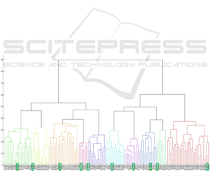
The second part of the process is to find, in each

cluster, the best performer, that is the index with the

highest Sharpe ratio, over the same learning period.

Figure 2 below exemplifies the process for the first

time-step 𝑡=0, May 1

, 2017.

Then, we build the portfolio composed by 𝜃

indices that are the “winners” of each cluster. The

portfolio is equally weighted. Finally, we run the

portfolio for the out-of-sample period [𝑡, 𝑡  𝜐 and

store the realized returns.

This process is repeated every 𝜐, in our base case

monthly, until the end of our sample period.

To test whether the clustering technique brings

diversification benefits in our CMOM portfolio, we

build a benchmark portfolio (MOM) that invests, at

each time-step 𝑡, to the 𝜃 indices that performed best

over the entire universe of available indices during

the same learning period [𝑡 − 𝜏, 𝑡), equally-weighted.

We expect this MOM portfolio to be highly

concentrated into one or a few ARP strategies at each

time-step, as the indices from different providers that

capture the same risk premium should perform

similarly, at least in theory.

In order to test if the performance persistence adds

value, we also build as benchmark the EW portfolio:

at each time-step, the ARP indices are classified into

the 𝜃 clusters as in CMOM. Then, we equally-weight

all the components of each cluster to build 𝜃 (in our

case 10) representative subindices. Finally, we invest,

again equally-weighted, into these subindices. Note

that, in this case, each cluster has the same weight,

regardless of the number of indices that compose it.

Additionally, we build 1,000 random portfolios:

starting at 𝑡=0, at each time-step 𝑡, each portfolio

selects, at random, 𝜃 ARP indices from the universe

available. Then, it invests equally-weighted on them

during the same out-of-sample period [𝑡, 𝑡  𝜐. This

random selection is performed with 𝜐 frequency until

the end of our sample September 28

, 2023. To make

the results more comparable to existing, investible

products, we simulate a 0.15% transaction cost every

time that a portfolio disinvests from an index between

two time-steps (i.e. if an index is present at 𝑡−1 but

not at 𝑡).

In a second test, we compare the results of the

CMOM, MOM and EW portfolios with 8 existing

ARP asset manager funds. In this case, we leverage

the portfolios’ weights at each time-step to achieve a

Figure 2: Cluster-momentum portfolio construction process at 𝑡=0 (May 1

, 2017).

FEMIB 2025 - 7th International Conference on Finance, Economics, Management and IT Business

178

target volatility of 𝜎



=7% annualized, similar

to the funds’ average volatility.

Finally, for robustness tests, we build the CMOM,

MOM and EW portfolios and re-run the out-of-

sample backtests but modifying 𝜏, or 𝜐, or both.

5 RESULTS

In this section, the results of the out-of-sample

backtests are presented. First, we compare the

performance of the CMOM portfolio with the MOM

and EW benchmarks. We also include the 5

–

percentile coefficients of various performance

measures from the 1,000 random portfolios.

5.1 Portfolios’ Performance

Table 2 exhibits the portfolios’ out-of-sample

descriptive statistics and Figure 3 the portfolios’ path

over time. It is noticeable that both the CMOM and

MOM portfolios outperformed the EW passive

benchmark, as well as more than 95% of the random

portfolios, in terms of annual returns. MOM delivered

better returns than CMOM. However, MOM also

manifested more risk, in terms higher volatility,

negative skewness, kurtosis, CVaR and maximum

drawdown coefficients.

Consequently, this

outperformance is not translated into the risk-adjusted

measures. CMOM shows a lower Sharpe ratio than

MOM (0.58 vs. 0.68), while the former exhibits a

higher Calmar ratio (0.36 vs. 0.31). These results

suggest that, first, there is added value that can be

extracted from performance persistence in ARP (i.e.

chasing the most recent winners), and second, that the

clustering technique achieves its desired outcome:

provide diversification to reduce the portfolio’s risk.

5.2 Cluster-Momentum Strategy vs.

ARP Asset Manager Funds

As a second set of benchmarks, we compare the

results of our CMOM strategy and the MOM and EW

portfolios with 8 existing asset manager ARP funds.

As a reminder, the CMOM, EW and MOM portfolios

are levered to achieve, at each rebalancing, a

volatility target 𝜎



=7% annually. Interestingly, the

out-of-sample, realized portfolio’s volatility

𝜎



is slightly above 9% for CMOM and MOM,

showing a large volatility “overshooting” impact,

while it is of 6% for the EW case. The funds’

volatility is, on average, 8.03%. In terms of annual

return 𝜇



, the fund’s average is of 1.87% only, likely

below investor’s expectations but above the naïve

EW strategy. The CMOM and MOM strategies

outperformed most funds, not only in terms of annual

returns (only Fund 1 and Fund 3 are above CMOM,

while no fund is above MOM), but especially in risk-

adjusted terms, where only Fund 1 outperformed both

strategies. In this case of levered portfolios, MOM

shows a higher Sharpe ratio (SR) than CMOM but the

latter still outperforms in terms of Calmar (CR).

It also exhibits lower (negative) skewness and

kurtosis coefficients. Another interesting result is

that, while the volatility of CMOM (9.36%) is larger

than most funds (8.12% on average), its maximum

drawdown (-15.40%) is lower, in absolute terms, than

all funds except Fund 1 and Fund 2. This is not the

case for MOM or even EW, whose MaxDD are

around 10 pp. larger (in absolute terms). Once again,

the benefits from diversification due to the clustering

Table 2: Portfolios’ out-of-sample descriptive statistics

𝜇



𝜎



𝑆𝑅 𝐶𝑅 𝑠𝑘𝑒𝑤. 𝑘𝑢𝑟𝑡. 𝐶𝑉𝑎𝑅



𝑀𝑎𝑥𝐷𝐷 𝑆𝑡𝑎𝑟𝑡 𝐷𝑢𝑟. 𝑅𝑒𝑐.

CMOM 2.33% 3.98% 0.58 0.36 -2.88 31.19 -0.63% -6.47% 07.03.23 7

EW 0.06% 2.47% 0.02 0.01 -2.71 20.55 -0.44% -9.06% 05.01.18 573

MOM 3.84% 5.61% 0.68 0.31 -3.50 45.40 -0.90% -12.26% 05.01.18 266 669

–

ct. 2.01% 3.23% 0.58 0.30 - - -0.50% -5.85% - - -

𝜇



: annual realized portfolio return; 𝜎



: annualized portfolio volatility; 𝑆𝑅 : Sharpe ratio; 𝐶𝑅: Calmar ratio; 𝑠𝑘𝑒𝑤. :

skewness coefficient; 𝑘𝑢𝑟𝑡. : excess kurtosis coefficient; 𝐶𝑉𝑎𝑅



: Conditional Value-at-Risk at 95% confidence level;

𝑀𝑎𝑥𝐷𝐷: maximum drawdown; 𝑆𝑡𝑎𝑟𝑡: maximum drawdown’s start date; 𝐷𝑢𝑟. : drawdown’s duration from peak to trough

(in days); 𝑅𝑒𝑐. ∶ drawdown’s recovery duration from trough to previous peak (in days). 5

-pct. Refers to the 5

– percentile

est coefficient of each measure. The out-of-sample investment period spans from 01.05.2017 to 28.09.2023.

The average fund’s realized volatility is 8.03%. We set

the target volatility at 7% as we expect some degree of

“volatility overshooting” out-of-sample. Anderson,

Bianchi and Goldberg (2014) show that leverage has a

negative impact on Sharpe ratio even without considering

transaction costs, via the “covariance term”.

Another result not reported here is that MOM tends to

show highly concentrated positions into the same ARP

strategy, while this is not the case for CMOM.

Introducing the Cluster-Momentum Portfolio in Alternative Risk Premia Investing

179

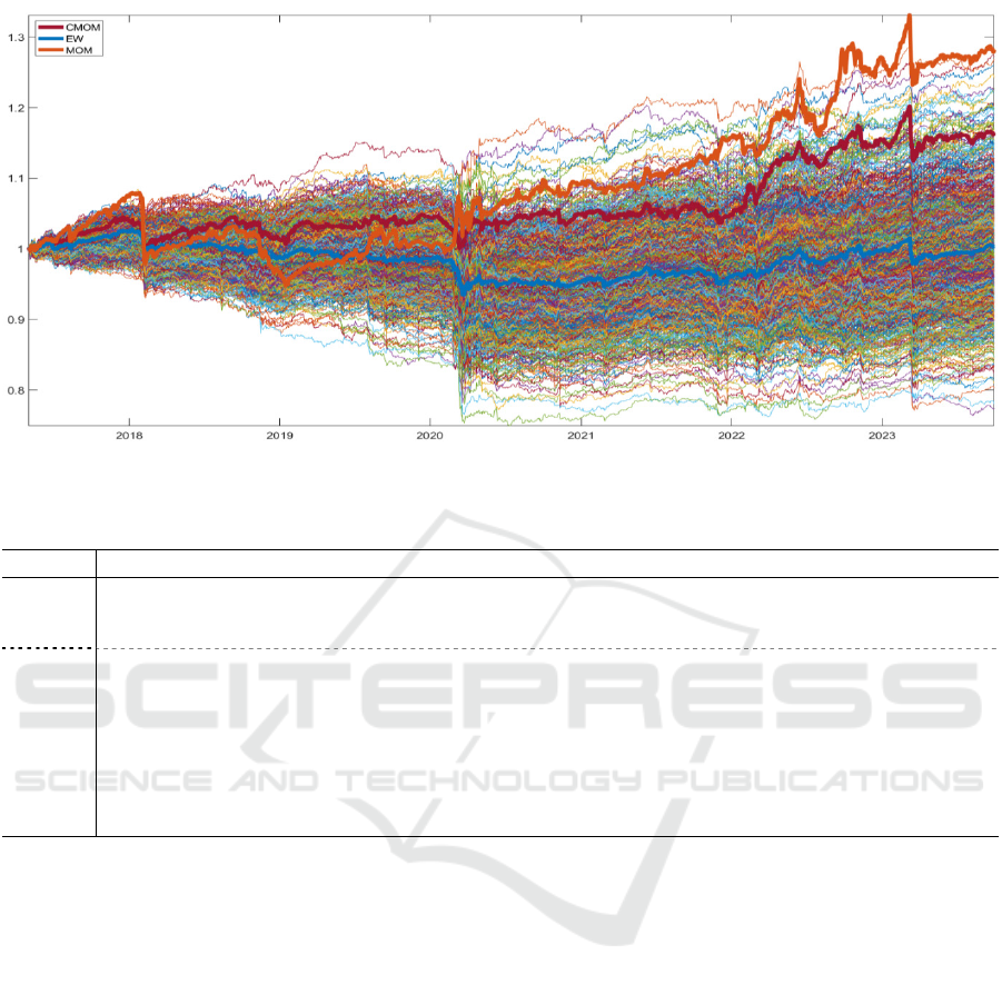
Figure 3: Portfolios’ path over the out-of-sample period.

Table 3: Levered portfolios’ and ARP asset manager funds’ out-of-sample descriptive statistics.

𝜇



𝜎



𝑆𝑅 𝐶𝑅 𝑠𝑘𝑒𝑤. 𝑘𝑢𝑟𝑡. 𝐶𝑉𝑎𝑅



𝑀𝑎𝑥𝐷𝐷 𝑆𝑡𝑎𝑟𝑡 𝐷𝑢𝑟. 𝑅𝑒𝑐.

CMOM 4.47% 9.36% 0.48 0.29 -2.51 31.78 -1.49% -15.40% 15.12.17 583 1079

EW -0.93% 5.97% -0.16 -0.04 -2.62 19.00 -1.08% -25.63% 05.01.18 573

MOM 5.67% 9.26% 0.61 0.24 -4.00 58.67 -1.50% -23.74% 05.01.18 266 939

Fund 1 5.56% 8.30% 0.67 0.41 -0.88 7.26 -1.35% -13.44% 18.02.20 20 191

Fund 2 3.07% 7.33% 0.42 0.22 -0.93 7.19 -1.13% -13.80% 17.01.20 45 209

Fund 3 4.85% 12.39% 0.39 0.12 -0.16 2.46 -1.82% -41.25% 31.01.18 743 1113

Fund 4* 2.52% 6.44% 0.39 0.13 -1.07 7.23 -1.00% -19.40% 25.01.18 726 1210

Fund 6 2.36% 10.81% 0.22 0.09 -0.50 3.52 -1.59% -24.92% 17.12.19 228

Fund 5 -0.02% 6.52% 0.00 0.00 -0.71 5.20 -1.06% -25.80% 26.01.18 804

Fund 7 -0.24% 7.79% -0.03 -0.01 0.41 8.37 -1.11% -31.00% 19.06.17 908

Fund 8 -3.15% 5.40% -0.58 -0.11 -0.70 5.97 -0.86% -28.68% 15.12.17 592

𝜇



: annual realized portfolio return; 𝜎



: annualized portfolio volatility; 𝑆𝑅 : Sharpe ratio; 𝐶𝑅: Calmar ratio; 𝑠𝑘𝑒𝑤.:

skewness coefficient; 𝑘𝑢𝑟𝑡.: excess kurtosis coefficient; 𝐶𝑉𝑎𝑅



: Conditional Value-at-Risk at 95% confidence level;

𝑀𝑎𝑥𝐷𝐷: maximum drawdown; 𝑆𝑡𝑎𝑟𝑡: maximum drawdown’s start date; 𝐷𝑢𝑟. : drawdown’s duration from peak to trough

(in days); 𝑅𝑒𝑐. ∶ drawdown’s recovery duration from trough to previous peak (in days). The out-of-sample investment

eriod spans from 01.05.2017 to 28.09.2023. *Fund 4 start date is 18.10.2017.

classification are present in our CMOM strategy.

Another intriguing result is the high skewness,

kurtosis and CVaR coefficients that our CMOM and

MOM portfolios show with respect to the values from

the funds.

Finally, it is worthwhile remembering that these 8

funds are all ARP asset manager funds that were

launched before May 2017 (except Fund 4, whose

start date is October 2017) and were still alive by

September 2023. There were ARP asset manager

funds that did not survive the 2018-2020 period of

underperformance of the ARP industry. Therefore,

there can be some “survivorship bias” in the sample

of funds and, if those “dead” funds were to be

included, it is likely that these ones would have also

underperformed.

To sum up, both the CMOM and MOM strategies

delivered very competitive results when compared to

the existing, investible funds, while the CMOM still

showed signs of risk-reduction with respect to MOM,

especially in terms of drawdown.

5.3 Robustness Tests: Modifying 𝝉

and 𝝊

As robustness tests, we build the same CMOM and

MOM portfolios but modifying the learning window

𝜏=



3,6,12



months and the rebalancing frequency

𝜐=



1,3



months (i.e. monthly or quarterly

FEMIB 2025 - 7th International Conference on Finance, Economics, Management and IT Business

180

rebalancing). Table 4 presents the results for all

combinations.

The results show that, not only

modifying parameters does not worsen the

performance of both the CMOM and MOM strategies

but it improves it in almost all combinations.

CMOM

appears to be more resilient to parameter

modifications, as the 3x1 MOM strategy is the only

combination that suffers a negative annualized return.

Another observation is that all quarterly rebalanced

portfolios outperform their monthly rebalanced

counterparts. Some combinations, such as the 3x3 in

CMOM and MOM and the 6x3 in MOM achieve

annualized returns above 10% with a similar level of

volatility. These results suggest that the CMOM

strategy is not negatively affected by the arbitrary

choice of the learning window and rebalancing

frequency parameters. In fact, the 12x1 base case

seems to be the portfolio with worst returns among all

combinations, and these ones were competitive when

compared to the asset manager funds. The benchmark

MOM portfolio seems to be more sensitive to

parameter modifications.

6 CONCLUSIONS

The selection and allocation of ARP is a challenging

task. IBs provide their own internal classifications

which can be different from one to another.

Moreover, each provider has its own cooking recipe

for each specific strategy, making two ARP indices

from the same strategy behave very differently in

some cases. On the other side, ARP that are

uncorrelated during quiet periods can become highly

correlated during market drawdowns, showing a

contagion effect. These and other complexities from

ARP investments must be considered when building

and managing portfolios.

In this article, we present a purely quantitative

approach that uses unsupervised hierarchical

clustering to achieve diversification, and then

allocates to the best performers among each of the

clusters, relying on some performance persistence

among ARP. This portfolio is backtested out-of-

sample and compared against a set of internal

benchmarks and existing asset manager ARP funds.

The results suggest that such a strategy would

have provided solid returns over the investment

period with a limited risk thanks to the benefits from

diversification achieved with the clustering

technique. Moreover, this portfolio shows resilience

to parameter modifications such as the learning

window or the rebalancing frequency. Strong

performance persistence appears to be present among

ARP, from which investors can profit from.

Furthermore, diversification through clustering

ensures that the portfolio won’t be too concentrated

into one or few ARP strategies, resulting into a

reduced risk without resigning from long-term

performance. These encouraging results should

incentivise researchers and practitioners to explore

further on the topic. For instance, it could be tested

whether increasing the number of clusters to have

more components in the portfolio, or picking more

Table 4: Out-of-sample descriptive statistics of portfolios with varied learning window and rebalancing frequency

𝜇



𝜎



𝑆𝑅 𝐶𝑅 𝑠𝑘𝑒𝑤. 𝑘𝑢𝑟𝑡. 𝐶𝑉𝑎𝑅



𝑀𝑎𝑥𝐷𝐷 𝑆𝑡𝑎𝑟𝑡 𝐷𝑢𝑟. 𝑅𝑒𝑐.

CMOM

12x1 4.47% 9.36% 0.48 0.29 -2.51 31.78 -1.49% -15.40% 15.12.17 583 1079

12x3 6.75% 9.67% 0.70 0.42 -2.31 27.41 -1.58% -15.96% 10.09.18 399 893

6x1 4.17% 9.24% 0.45 0.13 -2.67 22.78 -1.56% -31.96% 13.09.18 390 919

6x3 8.18% 9.75% 0.84 0.29 -2.42 24.01 -1.57% -28.31% 29.07.19 166 648

3x1 5.37% 9.12% 0.59 0.37 -1.95 20.90 -1.43% -14.44% 07.03.23 7 137

3x3 12.39% 8.90% 1.39 0.65 -0.90 9.84 -1.36% -19.10% 13.12.19 68 176

MOM

12x1 5.67% 9.26% 0.61 0.24 -4.00 58.67 -1.50% -23.74% 05.01.18 266 939

12x3 6.75% 9.67% 0.70 0.42 -2.31 27.41 -1.58% -15.96% 10.09.18 399 893

6x1 6.66% 9.96% 0.67 0.29 -2.42 20.48 -1.66% -22.82% 19.01.18 542 857

6x3 11.69% 9.78% 1.20 1.03 -2.02 18.41 -1.61% -11.37% 19.01.18 14 377

3x1 -0.33% 9.73% -0.03 -0.01 -2.17 20.32 -1.60% -29.21% 19.01.18 549

3x3 10.33% 9.65% 1.07 0.46 -1.16 13.74 -1.49% -22.22% 22.01.18 354 581

𝜇



: annual realized portfolio return; 𝜎



: annualized portfolio volatility; 𝑆𝑅 : Sharpe ratio; 𝐶𝑅: Calmar ratio; 𝑠𝑘𝑒𝑤. :

skewness coefficient; 𝑘𝑢𝑟𝑡.: excess kurtosis coefficient; 𝐶𝑉𝑎𝑅



: Conditional Value-at-Risk at 95% confidence level;

𝑀𝑎𝑥𝐷𝐷: maximum drawdown; 𝑆𝑡𝑎𝑟𝑡: maximum drawdown’s start date; 𝐷𝑢𝑟. : drawdown’s duration from peak to trough

(in days); 𝑅𝑒𝑐. ∶ drawdown’s recovery duration from trough to previous peak (in days). The out-of-sample investment

eriod s

ans from 01.05.2017 to 28.09.2023. *Fund 4 start date is 18.10.2017.

Introducing the Cluster-Momentum Portfolio in Alternative Risk Premia Investing

181

than one index in each cluster for the same purpose,

could add any value. In this article, we used

hierarchical clustering with the Ward method, but

other clustering techniques might be more

appropriate. In the same vein, the performance

measure to rank the underlyings could be another one

than the Sharpe ratio that was used here. All these are

just examples of many additional tests that can be

done, but that are left for further research.

REFERENCES

Anderson, R. M., Bianchi, S. W., & Goldberg, L. R. (2014).

Determinants of levered portfolio performance.

Financial Analysts Journal, 70(5), 53-72.

Blin, O., Ielpo, F., Lee, J., & Teiletche, J. (2021).

Alternative risk premia timing: A point-in-time macro,

sentiment, valuation analysis. Journal of Systematic

Investing, 1(1), 52-72.

Bruder, B., Kostyuchyk, N., & Roncalli, T. (2022). Risk

parity portfolios with skewness risk: An application to

factor investing and alternative risk premia. arXiv

preprint arXiv:2202.10721.

Carhart, M. M. (1997). On persistence in mutual fund

performance. The Journal of finance, 52(1), 57-82.

Fama, E. F., & French, K. R. (1993). Common risk factors

in the returns on stocks and bonds. Journal of financial

economics, 33(1), 3-56.

Fung, W., & Hsieh, D. A. (2004). Hedge fund benchmarks:

A risk-based approach. Financial Analysts Journal,

60(5), 65-80.

Gorman, S. A., & Fabozzi, F. J. (2021a). The ABC’s of the

ARP: understanding alternative risk premium. Journal

of Asset Management, 22, 391-404.

Gorman, S. A., & Fabozzi, F. J. (2021b). The ABC’s of the

alternative risk premium: academic roots. Journal of

Asset Management, 22, 405-436.

Gorman, S. A., & Fabozzi, F. J. (2022). Workhorse or

Trojan Horse? The Alternative Risk Premium

Conundrum in Multi-Asset Portfolios. Journal of

Portfolio Management, 48(4).

Hamdan, R., Pavlowsky, F., Roncalli, T., & Zheng, B.

(2016). A primer on alternative risk premia. Available

at SSRN 2766850.

Jorion, P. (2021). Hedge funds vs. alternative risk premia.

Financial Analysts Journal, 77(4), 65-81.

Kuenzi, D. E. (2020). Sources of Return Dispersion in

Alternative Risk Premia. The Journal of Alternative

Investments, 22(4), 26-39.

Monarcha, G. (2019). Alternative Risk Premia. August

2019. Orion Financial Partners.

Monarcha, G. (2020). Alternative Risk Premia. February

2020. Orion Financial Partners.

Naya, F., Rrustemi, J., & Tuchschmid, N. S. (2023a).

Alternative Risk Premia and Market Drawdowns: A

Performance Review. Journal of Beta Investment

Strategies, 14(2).

Naya, F., Rrustemi, J., & Tuchschmid, N. S. (2023b).

Incorporating alternative risk premia into balanced

portfolios: is there any added value? Journal of

Systematic Investing, 3(1), 1-13.

Naya, F. and Tuchschmid, N. S. (2019). Alternative Risk

Premia: Is the Selection Process Important? The

Journal of Wealth Management, 22 (1) 25-38.

Scherer, B. (2020). Alternative risk premia: contagion and

portfolio choice. Journal of Asset Management, 21(3),

178-191.

Suhonen, A., M. Lennkh, and Perez, F. (2017). Quantifying

Backtest Overfitting in Alternative Beta

Strategies. The Journal of Portfolio Management 43 (2):

90–104.

Suhonen, A., & Lennkh, M. (2021). Here in the Real World:

The Performance of Alternative Beta. Journal of

Systematic Investing, 1(1).

Suhonen, A., & Vatanen, K. (2023). Does Alternative Risk

Premia Diversify? New Evidence for the Post-

Pandemic Era. The Journal of Portfolio Management

(Forthcoming).

FEMIB 2025 - 7th International Conference on Finance, Economics, Management and IT Business

182