Deep Learning Characterization of Volatile Organic Compounds with

Spectrometer-on-Card

Ander Cejudo

1,2 a

, Markel Arrojo

1 b

, Miriam Guti

errez

1,3 c

, Karen L

opez-Linares

1,4 d

Hossam Haick

5 e

, Iv

an Mac

ıa

1,4,6 f

and Cristina Mart

ın

1,2,4 g

Fundaci

on Vicomtech, Basque Research and Technology Alliance (BRTA), Mikeletegi 57,

20009 Donostia-San Sebasti

an, Spain

Faculty of Engineering, University of Deusto, Avda. Universidades, 24, Bilbao 48007, Spain

Universidad Rey Juan Carlos, Cam. del Molino, 5, 28942 Fuenlabrada, Spain

BioGipuzkoa Health Research Institute (Bioengineering Area), eHealth Group, 20014 Donostia-San Sebasti

an, Spain

Department of Chemical Engineering and the Russell Berrie Nanotechnology Institute, Technion,

Israel Institute of Technology, Haifa 3200003, Israel

Computational Intelligence Group, Computer Science Faculty, University of the Basque Country, UPV/EHU, Spain

Keywords:

Exposome, Volatile Organic Compounds, Environment Characterization, Artiﬁcial Intelligence, Deep

Learning, Recurrent Neural Networks.

Abstract:

The exposome encompasses all environmental exposures that affect internal biological processes throughout

a person’s life, inﬂuencing health outcomes. Among these exposures, volatile organic compounds (VOCs)

are particularly signiﬁcant, as they are closely related to respiratory issues, cardiovascular diseases, cancer,

and other health conditions. Detecting some of them is therefore critical for assessing environmental impacts

on health. In this study, we use a low-cost, highly portable SPectrometer-On-Card (SPOC) device designed

to characterize complex mixtures by separating VOCs through its layers. The device was previously tested

to detect VOCs in controlled laboratory conditions. Hereby, we explore artiﬁcial intelligence algorithms to

identify patterns in the signals captured by the SPOC in closer to real-word conditions. Speciﬁcally, we focus

on two different use cases including direct exposure to a VOC source and indoors versus outdoors signal

recognition. Our top-performing model, a recurrent neural network, achieves accuracies of 92,4% and 97,2%

for each use case, respectively, effectively identifying exposures in the ﬁrst case and correctly classifying

87,5% of exposures in the second. These results demonstrate the potential of our methodology applied to

SPOC data for broader health-related applications, such as detecting incomplete combustions, identifying

diseases like cancer through exhaled breath, and detecting leaks from industrial plants.

1 INTRODUCTION

The concept of exposome is essential for understand-

ing health, as it encompasses the totality of environ-

mental exposures and their effects on internal biolog-

ical processes (Vermeulen et al., 2020). This holis-

tic perspective shows how diverse exposures (rang-

ing from chemicals to lifestyle factors) interact with

genetic predispositions to inﬂuence health outcomes

https://orcid.org/0000-0001-7944-2706

https://orcid.org/0009-0005-1099-7814

https://orcid.org/0000-0002-6692-9934

https://orcid.org/0000-0002-4800-6052

https://orcid.org/0000-0002-2370-4073

https://orcid.org/0000-0003-0448-7840

https://orcid.org/0000-0002-3919-2738

(Erzin and G

oks

uz, 2021; Danieli et al., 2024).

Among these chemicals, the study of volatile organic

compounds (VOCs) is particularly signiﬁcant, given

their prevalence in both natural and anthropogenic en-

vironments and their implications for public health

(Li et al., 2020; Zhang et al., 2024).

VOCs are produced by both natural sources (e.g.

vegetation) (Katsouyanni, 2003) and human activity.

Burning fossil fuels, solvents in industrial processes

like petroleum distribution and storage, and motor

vehicle fumes (particularly in cities with heavy traf-

ﬁc) are the main human-caused sources of VOCs (El-

bir et al., 2007; Wang and Zhao, 2008). Their pres-

ence in the air poses signiﬁcant health risks, as expo-

sure to VOCs has been linked to various adverse ef-

fects. These include allergies, respiratory issues like

asthma, chronic obstructive pulmonary disease, and

Cejudo, A., Arrojo, M., Gutiérrez, M., López-Linares, K., Haick, H., Macía, I. and Martín, C.

Deep Learning Characterization of Volatile Organic Compounds with Spectrometer-on-Card.

DOI: 10.5220/0013210300003938

Paper published under CC license (CC BY-NC-ND 4.0)

In Proceedings of the 11th International Conference on Information and Communication Technologies for Ageing Well and e-Health (ICT4AWE 2025), pages 197-207

ISBN: 978-989-758-743-6; ISSN: 2184-4984

197

irritation of the airways as a result of tropospheric

ozone generation (Tanaka et al., 2000). More severe

health issues like cancer, leukemia, and even mortal-

ity have been related to VOC exposure (Dutta et al.,

2018; Sun et al., 2016). The negative effects of VOCs

on human health depend on both the concentration

and the duration of the exposure (Soni et al., 2018).

The gold standard for VOC detection is gas

chromatography-mass spectrometry (GC–MS)

(Langford et al., 2014). This technique allows the

differentiation, identiﬁcation, and quantiﬁcation of

different VOCs in a sample. The sample is introduced

into the gas chromatograph, where the VOCs are

separated. A detector measures the quantity of each

ion, and the resulting spectrum is compared with a

reference library to identify the VOCs (Dincer et al.,

2006). However, this technology requires a labora-

tory, which is not always available or affordable. The

standard methodology for VOC detection is expen-

sive, energy-inefﬁcient, and slow, requiring around

20 to 40 minutes for analysis completion (Fialkov

et al., 2020). To bring the compound samples to the

laboratory, adsorption tubes are required (Ho et al.,

2018; Li et al., 2004). These tubes adsorb compounds

onto an adsorbent material for transport. During

this process, the compounds can undergo changes

due to humidity, oxidant exposure, or incomplete

desorption, which may alter the sample (Kumar

and V

ıden, 2007; Woolfenden, 2010). Then, the

contents of the tubes are released for analysis using a

technique called thermal desorption. Therefore, there

is a need to develop strategies to analyze VOCs in

situ, providing fast and high-resolution results.

For on-site VOC analysis, two main approaches

can be distinguished: individual VOC identiﬁcation

and non-target characterization. Devices designed for

the former approach require calibration for detect-

ing speciﬁc VOCs, which increases costs and limits

their ability to identify diverse compound mixtures

or a broader set of VOCs. In contrast, non-target

characterization devices, such as electronic noses (e-

noses) are more suited for detection, where the spe-

ciﬁc VOCs or mixtures of compounds are unknown

(Rabehi et al., 2024). These devices are usually

equipped with an array of cross-reactive sensors that

generate unique responses when exposed to various

complex mixtures of chemicals. These responses are

used to extract different patterns from the signals,

usually using unsupervised learning algorithms, be-

ing able to differentiate between groups and allow-

ing for applications such as early screening of various

cancers (Machado et al., 2005), lung diseases such as

pneumonia and upper respiratory tract infections (Per-

saud, 2005), diabetes (Saasa et al., 2019) or identiﬁ-

cation of bacterial pathogens (Lai et al., 2002). Al-

though e-noses are sensitive to VOCs mixture pres-

ence, they cannot identify speciﬁc VOCs within the

detected patterns (Smolander, 2003).

Recent advancements have led to the development

of a miniaturized spectrometer device (SPectrometer-

On-Card, SPOC) aimed at characterizing complex

mixtures containing unknown VOCs while also pro-

viding the ability to detect speciﬁc VOCs within these

mixtures. This is achieved through a multi-layer de-

sign, which separates VOCs as the air ﬂows through

the layers. However, this device is still a prototype

and has only been used for mixture characterization

and speciﬁc VOC detection in a controlled laboratory

environment at Technion (Israel Institute of Technol-

ogy) facilities Maity et al. (2022); more complex mix-

ture characterization in open-air environments has not

yet been conducted with this device.

The main objective of this work is to analyze the

potential of artiﬁcial intelligence (AI) techniques to

differentiate signals captured by the SPOC in two,

closer to real-world, environments. The unique fea-

tures of the SPOC for non-target VOC detection, com-

bined with the proposed methodology for signal clas-

siﬁcation may allow to analyze diverse compound

mixtures without being limited to a speciﬁc set of

VOCs. The results will highlight the potential of

this technology, combined with a novel AI approach,

to analyze diverse compound mixtures without being

limited to a speciﬁc set of VOCs.

The structure of the paper is organized as fol-

lows. In section 2, we delve into the previous re-

search conducted on the analysis of volatile organic

compounds. Section 3, provides an explanation of

the device used for data captured, the use cases con-

sidered in this study and the deep learning approach

for environment characterization. Section 4 presents

and discusses the quantitative results obtained from

the experiments. Section 5 concludes the study by

summarizing the key ﬁndings.

2 BACKGROUND

There are many studies that detect speciﬁc VOCs and

their concentrations for air quality assessment. Won

et al. (2021) analyzed the concentrations of 24 VOCs

that are measured in underground shopping districts

in Korea using a Thermal Desorption–Gas Chro-

matography Mass Spectrometry (TD–GCMS) device.

The results indicated higher VOC concentrations in-

doors, identifying six sources of air pollution. Simi-

larly, the authors of (Scheepers et al., 2017) studied

the indoor air quality of a university hospital. Air

ICT4AWE 2025 - 11th International Conference on Information and Communication Technologies for Ageing Well and e-Health

198

samples were collected both indoors and outdoors us-

ing canisters and then these were analyzed with TD-

GCMS. The authors concluded that laboratory work

contributes substantially to indoor pollution, whereas

known outdoor sources do not signiﬁcantly affect in-

door air quality. Another study (Pang et al., 2019)

used a portable photoionization detector to charac-

terize up to eight VOCs in a laboratory environment,

showing that the concentration response increases lin-

early with the chemical concentrations tested.

Several works can be found in the state-of-the-art

that aim at the non-target characterization of air based

on VOC detection. Many of these works make use

of e-noses, which are particularly popular for provid-

ing distinguishable patterns for different VOC expo-

sures. One of the ﬁrst works that addressed the envi-

ronment characterization problem using e-noses was

conducted by Nicolas et al. (2000). They used the

response of a cross-reactive detector to monitor air

quality combined with principal components analy-

sis to classify different unknown air mixtures around

VOC emitting sources. Similar works use artiﬁcial

neural networks to identify patterns in data registered

from the pulp and paper industry (Deshmukh et al.,

2014). For example, Licen et al. (2020) used an e-

nose device to identify patterns with clustering and

self-organizing maps from different VOC mixtures in

the context of air quality. Furthermore, they validated

their ﬁndings by using ancillary data from a photoion-

ization detector that measures VOCs.

VOC characterization in air extends beyond air-

quality control and has proven valuable in other ﬁelds,

particularly in early-stage disease diagnosis, as ex-

haled air can provide valuable insights into metabolic

diseases (Li et al., 2023). For instance, Anzivino et al.

(2022) successfully used Principal Component Anal-

ysis (PCA) to cluster patients with head and neck can-

cer and rhinitis based on breath signals captured by an

e-nose device. Similarly, (Liu et al., 2021) proposed

a PCA-Singular Value Estimation ensemble learning

framework to cluster the 214 breath samples for early

lung cancer detection, achieving excellent results with

95,75% accuracy and 94,78% recall in their classiﬁ-

cation task.

While the non-target characterization of air has

been extensively researched ((Nicolas et al., 2000; Li-

cen et al., 2020)) and the application of AI is common

in this ﬁeld (Liu et al., 2023), to the best of our knowl-

edge, no prior studies have explored AI-enhanced

characterization using a portable, lightweight, and

cost-effective device capable of providing insights

into individual detection as well. Thereby, in this

work we aim to leverage a methodology based on

advanced signal processing and AI tools to disentan-

gle information coming from a multi-layered detector

that is able to characterize and differentiate complex

air mixtures.

3 MATERIALS AND METHODS

This section introduces the device used for data cap-

ture in two different use cases and the designed deep

learning-based pipeline for environment characteriza-

tion. Subsection 3.1 outlines the motivation behind

the SPOC device for VOC analysis, whereas subsec-

tion 3.2 details the two use cases selected for this

study. Finally, subsection 3.3 presents the methodol-

ogy for signal analysis using several machine learning

methods.

3.1 Spectrometer-on-Card

The SPectrometer-On-Card (SPOC) device, proto-

typed by Technion (Israel Institute of Technology),

is employed to detect and measure the presence

of VOCs in suspension. This innovative technol-

ogy utilizes a miniaturized, layer-based sensor ca-

pable of identifying complex molecular structures

through a hierarchically stacked geometrical conﬁg-

uration (HSGC). Each layer is composed of function-

alized graphene sensors printed on porous cellulose

sheets, with multiple layers stacked together (Maity

et al., 2022). This architecture could be thought of

as a miniaturized version of chromatography columns

(where the porosity of cellulose plays the main role)

and mass spectrometer (where the array of sensors is

responsible for identifying unknown compounds).

As a mixture of compounds ﬂows from the ﬁrst

to the last layer, molecules are differentiated through

two mechanisms: molecular size (due to the porous

nature of the layers) and chemical afﬁnity (due to lig-

ands bound to the functionalized sensors). Molecules

with lower adsorption or weaker chemical afﬁnity

travel faster and reach the sensors earlier, generating a

multi-peak resistance proﬁle. Each peak corresponds

to a distinct molecule from the original mixture, as

illustrated in Figure 1.

This spatio-temporal detection at each layer gen-

erates a multidimensional signal as shown in Figure 2,

enabling multi-channel detection and analysis. Each

layer (or channel) captures different aspects of the

evaluated mixture, reﬂecting its diverse properties.

3.2 Experimental Setup

Two experiments (see Figure 3) are designed to differ-

entiate environments based on the presence of various

Deep Learning Characterization of Volatile Organic Compounds with Spectrometer-on-Card

199

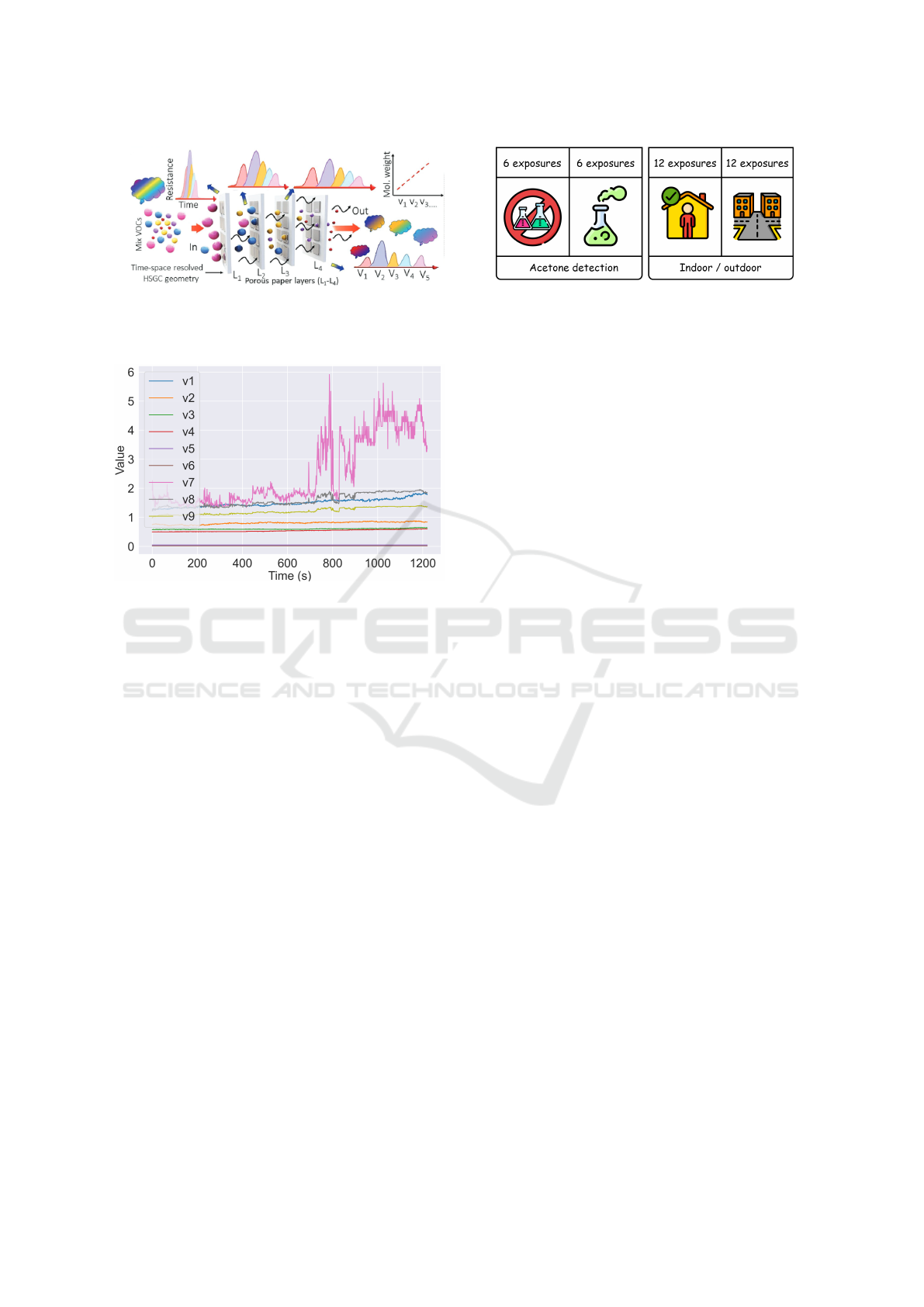
Figure 1: Graphical representation of the SPOC mechanism

for identifying different VOCs in a mixture. Figure taken

from Maity et al. (2022).

Figure 2: Example of raw signal captured in open air. The

x-axis represents the time interval of exposure (sampling

frequency was established to 1 Hz, hence the signals rep-

resent information from 1200 s. The y-axis represents the

resistance signal in omhs in each of the 8 channels.

VOC mixtures. The ﬁrst experiment involves expos-

ing the SPOC to a semi-controlled environment with

a well-known source of VOCs (acetone). In contrast,

exposures without a direct VOC-emitting source are

captured in an indoor environment for artiﬁcial intel-

ligence (AI)-based characterization. The objective of

the ﬁrst use case is to see the capabilities of the pro-

posed AI-driven approach to differentiate patterns in

the signals in an environment where there is a clear

presence of VOCs combined with a possible pres-

ence of unknown mixtures of compounds. This is

a more complex situation than a laboratory environ-

ment, which typically has clean air containing only

the selected compounds. A total of 12 samples have

been collected, each lasting about 30 minutes. Six of

these samples are exposed to an acetone dissolution

inside a closet, while the remaining six were exposed

to indoor air at a desk in the ofﬁce. (see Table 1 for a

detailed description).

The second use case is designed to assess the ca-

pabilities of the proposed AI-based methodology (see

subsection 3.3) in a scenario widely studied in the

state-of-the-art for indoor and outdoor environment

characterization (Vardoulakis et al., 2020). Previous

Figure 3: Representation of the two use cases considered

in this study and the number of exposures taken for each

environment.

works indicate that, in general, the concentration of

VOCs is higher indoors. For that reason, the readings

of the device should be differentiable in both environ-

ments. In this phase, exposures collected in an ofﬁce

environment are compared with those from a nearby

outdoor industrial area. The SPOC device was posi-

tioned at a designated ofﬁce desk for indoor sampling,

while the outdoor sampling area was located close to

the ofﬁce, near a lightly trafﬁcked road and alongside

a river. For this experiment a total of 24 samples are

collected, each taking approximately 20 minutes: 12

samples from outside and 12 from inside (Table 1).

These experiments are designed to evaluate the

deep learning-based methodology across two differ-

ent use cases in semi-controlled and uncontrolled en-

vironments. The ﬁrst use case is designed to evaluate

the characterization performance of the pipeline when

having a direct exposure to a VOC-emitting source.

In the second use case, the evaluation is carried with

signals obtained when the device is exposed to un-

known mixtures of compounds in both, indoor and

outdoor environment, as seen in previous works (Var-

doulakis et al., 2020). This second use case serves

to showcase the potential of the proposed methodol-

ogy for the characterization of environments closer to

real-world conditions.

3.3 Environment Characterization

Environment characterization is done through a time

series analysis of the exposures (E) captured in the

environments described in subsection 3.2 (Figure 3).

Each exposure ( j) with a duration of n seconds is di-

vided into windows (w) of size p (see equation (1)).

The whole exposure analysis process is depicted in

Figure 4,

E = {e

, ..., e

} (1)

W = {w

, ..., w

j(n−p+1)

, ..., w

m(n−p+1)

}

Then the window (w

i j

) is provided to the AI model

to assign a probability (p

) for the i-th window indi-

cating the resemblance to a certain environment. The

ICT4AWE 2025 - 11th International Conference on Information and Communication Technologies for Ageing Well and e-Health

200

Table 1: Data description of the acetone detection and indoor / outdoor environment characterization use cases. For each use

case, the features used to train the proposed artiﬁcial intelligence (AI) models are detailed after applying the sliding window.

Group Features

Acetone detection Indoor / outdoor

characterization

Yes No Total Indoor Outdoor Total

Count

# Exposures 6 6 12 12 12 24

# Variables 9 channels 9 channels

Duration (s)

Mean 1.821 1.823 1.822 1.502 1.215 1.358

Std 35,03 34,06 32,25 695,00 63,66 504,40

Min 1.772 1.793 1.772 524 1.022 524

Max 1.881 1.886 1.886 3.292 1.263 3.292

Window size 25 25

Step 1 1

Train

# Instances 7.120 7.171 14.291 10.662 9.457 20.119

# Exposures 4 4 8 7 8 15

Test

# Instances 3.662 3.600 7.262 7.056 4.827 11.883

# Exposures 2 2 4 5 4 9

proposed methodology is ﬂexible and can have a vary-

ing number of layers (l) as input.

AI : P

× P

→ [0, 1] (2)

= {v

, ..., v

} → AI(w

) = p

With the list of probabilities (P

) assigned to each of

the windows from the j-th exposure, the mean score

is obtained, indicating on average, the resemblance of

the whole exposure with respect to the speciﬁc envi-

ronment. Finally, the predicted label ( ˆc

) for the j-

th exposure is obtained by rounding the mean score

to either 0 or 1 (see equation (3)). Note that the

split of the exposure in smaller windows generates

a larger number of instances and smaller sequences.

This enables the training of more complex models,

such as recurrent neural networks (RNNs), and re-

quires a lower number of exposures for training. Sim-

ilar approaches have been proposed in previous works

for the classiﬁcation of long sequences with smaller

windows (Dietterich, 2002; Senthil and Suseendran,

2018; Etemad et al., 2020).

= {AI(w

)}

i=1

(3)

ˆc

= Round(Mean(P

))

The AI models considered for the environment

characterization task include several algorithms as

well as deep learning-based methods. The ﬁrst

group of machine learning methods includes: K-

Neares Neighbours (KNN), Support Vector Machine

(SVM), Decision Tree (DT), Stochastic Gradient De-

scent (SGD) and Neural Networks (NN) (Boateng

et al., 2020). The SVM classiﬁer contains a radial

basis function kernel. Note that these algorithms are

not able to have as input two-dimensional windows,

for that reason, the window size (p) is set to one.

This setting implies that the classiﬁcation is done for

each second, attending combinations between the val-

ues read for each of the layers and missing tempo-

ral patterns in the analysis. The second group of

models are based on recurrent neural networks RNNs

(Medsker et al., 2001), which consider large win-

dow sizes and are able to learn spatio-temporal pat-

terns in the signals. More speciﬁcally, three varia-

tions of RNNs are employed (see Figure 5): RNN,

Bidirectional RNN (BiRNN) and RNN with a built-

in attention mechanism (AttentionRNN). The RNN

is composed of Long Short-Term Memory (LSTM)

(Hochreiter, 1997) cells that are able to capture infor-

mation in further timesteps.

For the RNN, an additional set of parameters must

be speciﬁed such as the optimizer function, which de-

ﬁnes how the parameters are updated, the number of

epochs (i.e. the number of passes through the entire

dataset), dropout (i.e. randomly ignores the speci-

ﬁed percentage of neurons from the previous layer to

avoid overﬁtting) and the learning rate. In addition,

for the Adam optimizer (Bock and Weiß, 2019), β1

and β2 have to be set which are the exponential decay

rates for the ﬁrst and second moment estimates, re-

spectively. Finally, the batch size is also tuned which

deﬁnes the number of instances to introduce in the

network in each step within an epoch.

For the traditional machine learning algorithms,

python’s scikit-learn (Pedregosa et al., 2011) library

is used. In the case of NN, RNN, BiRNN and At-

tentionRN, keras (Gulli and Pal, 2017) is the frame-

work used for the implementation of the proposed

models. The hyperparameters of these deep learning-

based models are automatically adjusted with the Op-

Deep Learning Characterization of Volatile Organic Compounds with Spectrometer-on-Card

201

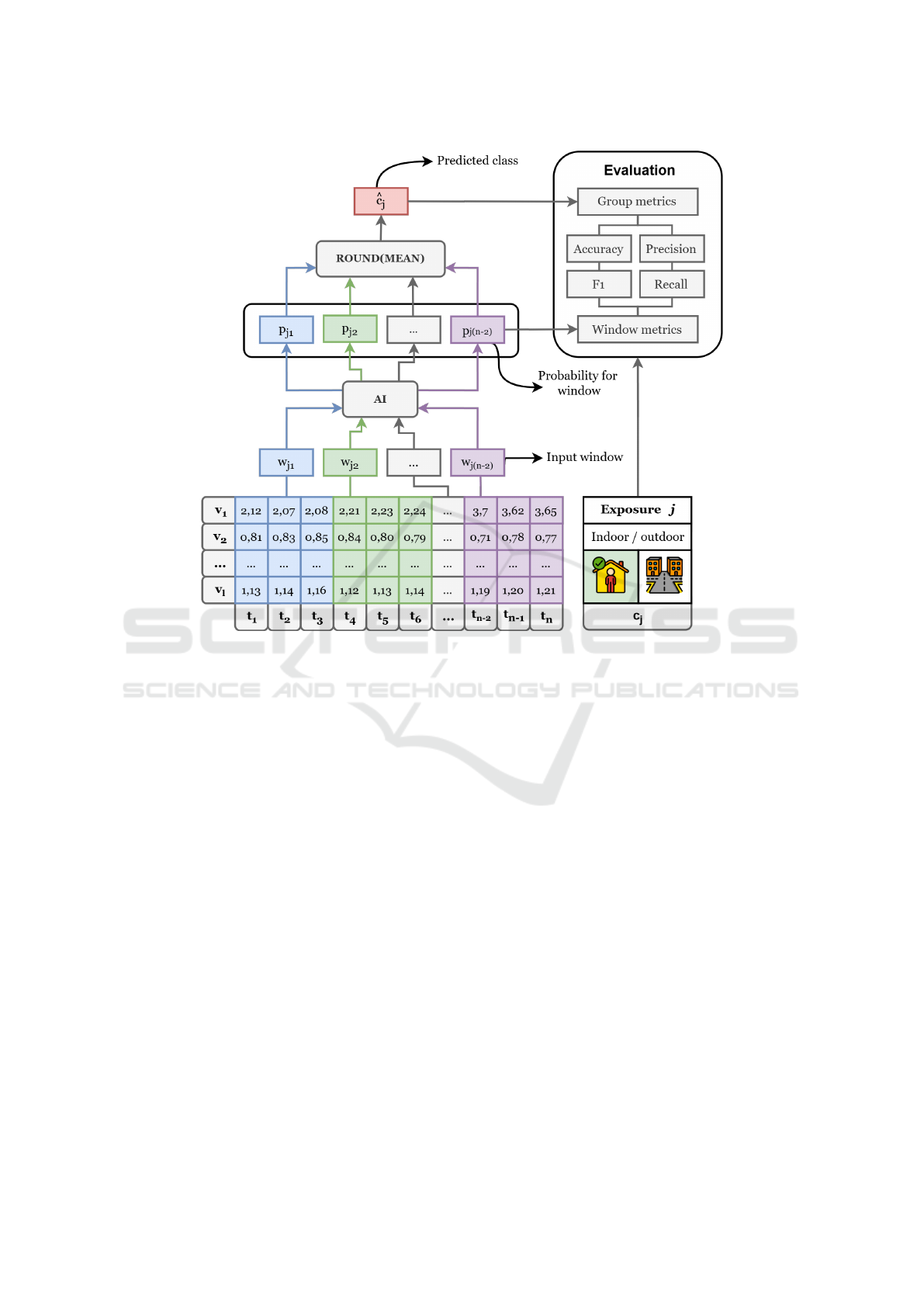
Figure 4: Diagram of the environment characterization process given an exposure. In this example, input data is divided

into windows of size three for indoor and outdoor classiﬁcation. For each window, an AI model assigns a probability of

resemblance to the outdoor environment. The mean and round functions are then applied to these probabilities to classify the

entire exposure. Evaluation metrics are used to compare the input and predicted data.

tuna (Akiba et al., 2019) framework. Among those

hyperparameters that are optimized by this frame-

work: window size, dropout rate, the RNN number

of neurons, number of feedforward layers, number of

neurons in each feedforward layer. Description of the

data used for the proposed AI models is shown in Ta-

ble 1 after selecting the best window size for the pro-

posed use cases.

3.4 Evaluation

The evaluation of the environment characterization

performance is done in three ways: window metrics,

group metrics and mean probabilities. For both, win-

dow and group metrics, the accuracy and F1 are com-

puted (Dalianis and Dalianis, 2018), being the max-

imum value 100%, which indicates a perfect charac-

terization. Both metrics measure how close the pre-

diction is to the current label. As the exposure is split

into smaller windows, each window is assigned the

same label as the whole exposure. That is, the smaller

windows come from the same environment as the ex-

posure. For each window, the accuracy and F1 scores

are computed, comparing the label of the window and

the label of the whole exposure.

For group metrics, the probabilities of all the win-

dows within the exposure are averaged and rounded,

comparing the predicted class of the exposure with the

actual class. Group metrics indicate the percentage of

exposures in the test set that are correctly classiﬁed.

Mean probabilities computed for the acetone detec-

tion use case are differentiated for label 1 (e.g. no

acetone exposure) and label 2 (e.g. acetone exposure)

exposures, obtaining the mean probability assigned

across all the windows inside the exposure. The same

happens for the second use case, where the exposures

captured indoors are assigned with label 1 and those

captured outdoors with label 2.

The selected evaluation scheme is 3-fold cross val-

idation (Berrar et al., 2019), which splits the data into

three folds, and at each time, two folds are used for

training and the remaining one for testing. This en-

sures that the results are not conditioned to the spe-

ciﬁc train/test data partition. For that reason, for each

ICT4AWE 2025 - 11th International Conference on Information and Communication Technologies for Ageing Well and e-Health

202

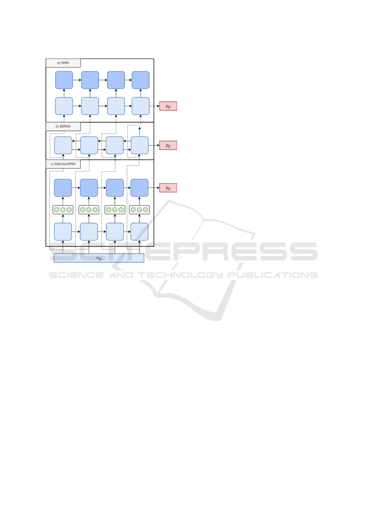
Figure 5: Representation of different recurrent neural net-

work architectures employed in this study: (a) RNN, (b)

BiRNN, and (c) AttentionRNN. For each experiment, one

of these architectures is selected independently and the

number of seconds in the input (p) is tuned to achieve the

best environment characterization performance. In this ex-

ample, the window size (p) is set to four. All the classiﬁers

have as input a window (w

) and as output a probability

). Note that the algorithms are not combined, but share

the same input and output format.

evaluation metric, the mean value and the standard de-

viation are provided. In addition, the data is stratiﬁed,

that is, in the test set half of the exposures are always

from the ﬁrst environment (label 1) and the other half

from the second environment (label 2).

4 RESULTS

This section presents the ﬁndings from the exper-

iments conducted for environment characterization.

First, in subsection 4.1 the performance of the pro-

posed methodology in characterizing environments

based on mixtures of VOCs is detailed, highlighting

key metrics such as accuracy for both use cases. Fol-

lowing this, in subsection 4.2 a comprehensive discus-

sion of these results is provided, contextualizing their

signiﬁcance and exploring potential implications for

future applications.

4.1 Environment Characterization

In this section, a set of experiments is presented

for environment characterization in two different use

cases: acetone detection and indoor/outdoor charac-

terization. The main objective is to see if the method-

ology depicted in Figure 4 is able to distinguish the

two environments. The characterization performance

for both use cases may differ as the ﬁrst one has a di-

rect source of VOC. Classiﬁcation results are shown

in Table 2.

Table 2 shows the classiﬁcation results by means

of window and group metrics for acetone detection

and indoor/outdoor characterization. For acetone de-

tection, the best mean window metrics are achieved

by the BiRNN model, with a maximum accuracy of

97,24% and a F1 of 97,25%. Group metrics show that

the four exposures of the test set are correctly clas-

siﬁed for the three RNN-based models, being able to

differentiate the two exposures that were exposed to

acetone. The results obtained by the BiRNN are close

to those obtained by the RNN model for the win-

dow metrics, with a 95,50% of accuracy and a F1 of

95,51%. Regarding the mean probability assigned to

those exposures exposed to an acetone source (label

2), the BiRNN model provides a 99,10% for the ex-

posures in the test set across the different folds, com-

pared to 93,91% achieved by RNN, showcasing a high

precision for BiRNN. This precision seems to affect

the mean probability for those cases where there is no

acetone source (label 1), being the lowest for RNN

with 2,73%.

A comparison of the window metrics between

RNN, the best RNN-based model, with NN, which

is the best model from those that have one as window

size, shows a relative increase in terms of mean ac-

curacy of 15,36% and 14,53% for mean F1. Group

metrics show that the mean accuracy for NN is 83,3%

whereas for RNN is 100%. Considering that the num-

ber of exposures in the test set is 3, on average, the NN

classiﬁes one or two exposures out of three whereas

the RNN is able to correctly characterize the three ex-

posures. These results indicate that the temporal pat-

terns of the signals have a high inﬂuence on the envi-

ronment characterization capabilities of the proposed

model.

For indoor / outdoor environments characteriza-

tion, the best score is also achieved by the BiRNN

with a mean accuracy of 92,37% and 92,38% in terms

Deep Learning Characterization of Volatile Organic Compounds with Spectrometer-on-Card

203

Table 2: Results for environment characterization through the classiﬁcation of the exposures in the test set. The scores for the

evaluation metrics are divided for each of two use cases shown in Figure 2 and given for the window and group metrics. The

best results for each use case are marked in bold.

Window metrics Groups metrics Mean probabilities

Use case Model Accuracy F1 Accuracy F1 Label 1 Label 2

Acetone detection

conditions

KNN 53,03% (±2,47) 50,79% (±19,36) 54,17% (±37,69) 43,33% (±30,15) 16,66% (±0,00) 17,00% (±0,00)

RBF SVM 61,06% (±15,47) 61,01% (±12,43) 54,17% (±37,69) 43,33% (±30,15) 39,04% (±0,00) 38,80% (±0,00)

Decision Tree 63,97% (±1,88) 62,52% (±5,58) 72,92% (±18,84) 66,67% (±0,00) 37,53% (±0,00) 66,67% (±0,10)

SGD 61,64% (±21,57) 60,75% (±15,57) 54,17% (±37,69) 43,33% (±30,15) 12,73% (±3,62) 31,51% (±10,86)

NN 84,29% (±9,27) 84,91% (±8,44) 83,33% (±19,46) 82,22% (±13,73) 18,65% (±27,30) 87,05% (±13,00)

RNN 95,50% (±7,68) 95,51% (±7,65) 100,00% (±0,00) 100,00% (±0,00) 2,73% (±4,51) 93,91% (±10,52)

BiRNN 97,24 % (± 4,75) 97,25% (±4,74) 100,00% (±0,00) 100,00% (±0,00) 4,49% (±7,78) 99,10% (±1,52)

AttentionRNN 90,45% (±9,65) 90,65% (±9,36) 100,00% (±0,00) 100,00% (±0,00) 3,93% (±5,28) 85,09% (±19,13)

Indoor / outdoor

characterization

KNN 65,44% (±13,29) 64,17% (±4,49) 66,67% (±24,62) 62,50% (±9,23) 52,20% (±0,00) 83,77% (±0,00)

RBF SVM 63,05% (±13,88) 61,58% (±5,05) 50,00% (±12,31) 48,57% (±6,33) 55,33% (±0,00) 82,21% (±0,00)

Decision Tree 59,45% (±12,29) 56,49% (±7,88) 66,67% (±0,00) 62,50% (±9,23) 65,11% (±0,59) 85,16% (±0,20)

SGD 67,01% (±14,66) 65,54% (±5,31) 66,67% (±24,62) 62,50% (±9,23) 46,04% (±8,99) 86,26% (±0,87)

NN 89,58% (±5,73) 89,68% (±5,55) 91,66% (±9,73) 91,53% (±6,33) 8,86% (±10,20) 86,24% (±14,49)

RNN 91,86% (±5,54) 91,87% (±5,54) 95,83% (±8,14) 95,77% (±6,29) 7,84% (±7,91) 89,91% (±8,49)

BiRNN 92,37% (±4,78) 92,38% (±4,77) 95,83% (±8,14) 95,77% (±6,29) 6,48% (±6,20) 89,65% (±7,12)

AttentionRNN 88,66% (±6,17) 88,71% (±6,10) 95,83% (±8,14) 95,77% (±6,29) 9,28% (±6,41) 84,70% (±9,95)

of mean F1. Group metrics achieve a mean score of

95,38% in terms of accuracy and 95,77% by means of

mean F1, which implies that from eight exposures in

the test set, on average, 7 to 8 of them are correctly

classiﬁed. These results are close to those obtained

by the RNN, with 91,86% and 91,87% of mean ac-

curacy and F1, respectively. The mean probability

assigned to outdoor exposures (label 2) is very sim-

ilar for both RNN and BiRNN, being the mean value

higher for the RNN with 89,91% compared to 89,65%

but the standard deviation is lower for BiRNN. For in-

door exposures (label 1) the mean probability is lower

for BiRNN with a 6,48% compared to the 7,84% pro-

vided by the RNN.

When comparing the best model that uses one as

window size (NN) and the best RNN-based model

(BiRNN), a relative increase of 3,11% is achieved in

terms of mean accuracy and 3,01% in terms of mean

F1. Group metrics for both NN show that, with a

mean accuracy of 91,66% and a standard deviation

of 9,73, at most one exposure is incorrectly classi-

ﬁed. These results, compared to those obtained in the

acetone detection use case, also show a difference in

performance when considering the time component of

the SPOC data, being higher for RNN-based models.

As a conclusion, the RNN-based models have

achieved a remarkable increase in performance com-

pared to those models that do not take into account the

time domain of the input data. In addition, the best

model has been BiRNN for both use cases, achiev-

ing a 95,25% mean accuracy for the acetone detec-

tion scenario. For the indoor and outdoor environ-

ment characterization use case the BiRNN achieves

a 92,37% of mean accuracy. In the acetone detec-

tion use case all the exposures are correctly classi-

ﬁed, whereas in the indoor and outdoor characteriza-

tion use case, only one exposure is incorrectly classi-

ﬁed. These results show the capabilities of the SPOC

device combined with the proposed methodology for

environment characterization. Optuna framework has

proven to be essential to adjust different hyperparam-

eters and optimize model performance, with the num-

ber of trials to 25 and the NSGA-III algorithm (Deb

and Jain, 2014) as the optimization function.

4.2 Discussion

This study proposes an AI-driven methodology that

incorporates deep learning techniques to character-

ize environments using signals captured by the SPOC

device under two different use cases: acetone detec-

tion and indoor / outdoor characterization. The ﬁrst

one has a known source of VOCs (acetone), and the

second one is exposed to lower concentration of un-

known mixtures of compounds. Although the ﬁrst

case directly exposes the device to acetone, other

VOCs may also be present in the air, with acetone

concentration being signiﬁcantly higher. Given the

high mean classiﬁcation accuracy of 97,24%, it would

be valuable to compare the signals from other VOCs

to analyze potential differences in the SPOC’s read-

ings.

The motivation for the second use case is sup-

ported by previous research reporting signiﬁcant dif-

ferences between indoor and outdoor environments,

with VOC concentrations generally being higher in-

doors (Vardoulakis et al., 2020). For this use case, the

model’s performance decreases by around ﬁve points

in terms of mean accuracy, which may be attributed to

the characterization of an uncontrolled environment

compared to the semi-controlled environment of the

ﬁrst use case. In contrast, when measurements are

taken in uncontrolled environments, along with the

presence of environmental noise, the concentration of

ICT4AWE 2025 - 11th International Conference on Information and Communication Technologies for Ageing Well and e-Health

204

VOCs may be signiﬁcantly reduced. Another factor

affecting accuracy could be situations where the in-

door and outdoor environments are not differentiable,

possibly due to cleaner indoor air or airﬂow from the

outside. Thus, exposure classiﬁcation errors may in-

dicate changes in the mixtures of VOCs in environ-

ments monitored by the SPOC device.

The comparison of results achieved by the models

in Section 4 primarily considers the mean scores of

the proposed metrics. Additionally, a paired t-test was

performed using the standard deviation across the dif-

ferent folds. The results provide no evidence of a sta-

tistically signiﬁcant difference in performance among

the recurrent neural network-based models. There-

fore, selecting the best model may vary depending

on the score for each use case, computational time,

and preferred mean probability. For example, in the

acetone detection use case, if better detection of pos-

itive cases is prioritized, the BiRNN performs better

(99,10%). However, if the goal is to monitor normal

environmental conditions and reduce false positives,

the RNN may be preferable with a mean probability

of 2,73%. In any case, RNN-based models signiﬁ-

cantly outperform those models limited to a window

size of one (p < 0, 005), demonstrating the advantages

of considering the time domain of the signals.

Future work should consider expanding the num-

ber of environments used for characterization and

evaluating the SPOC and the proposed methodology

on more complex tasks. A deeper analysis of the sig-

nals would be valuable to understand the inﬂuence of

each layer in the characterization process, as well as

any patterns indicative of speciﬁc VOCs, leveraging

the capabilities of this device compared to previous

approaches like the e-nose.

The proposed methodology has proven to be ef-

fective for environment characterization based on

VOC mixtures using just a few hours of data for

model training. This is achieved by splitting the expo-

sure into windows, generating thousands of instances

for training deep learning models. Additionally, this

solution can be used for real-time monitoring, provid-

ing a probability every second by analyzing the last

25 seconds of data. Therefore, this approach could

potentially be used for other air quality assessments

or the detection of speciﬁc health conditions based on

air from exhaled breath. The only requirement would

be to capture a few hours of data to retrain the model

for characterization, eliminating the need for calibra-

tion or new sensors. Then, the predictions could be

provided at each second, depending on the hardware

provided for the inference.

5 CONCLUSIONS

In this work, we propose and evaluate an AI-

based pipeline for environment characterization that

compares several machine learning and deep learn-

ing classiﬁers, including recurrent neural networks

(RNNs). To assess the capabilities of our approach,

we have captured SPectrometer-On-Card (SPOC)

data in two different use cases. In the ﬁrst use case,

this pipeline is used for the characterization of an en-

vironment with a direct source of VOC (acetone). In

the second use case, the evaluation is carried out in

indoor and outdoor environments (a common applica-

tion in the state-of-the-art), where the concentration

of unknown mixtures of compounds is lower com-

pared to the ﬁrst use case. With that aim, our approach

splits the signal into smaller windows and compares

different machine learning algorithms for environ-

ment classiﬁcation based on SPOC signals generated

as a response to the exposition of complex mixtures of

compounds. The probabilities for these windows are

averaged across the entire exposure and a ﬁnal predic-

tion is given. The results show that the bidirectional

recurrent neural network (BiRNN) achieves the best

performance with a 97,24% mean accuracy in win-

dow classiﬁcation and all the exposures are correctly

characterized. For indoor and outdoor characteriza-

tion use cases, a mean accuracy of 92,97% is achieved

for window classiﬁcation with seven exposures out of

eight correctly classiﬁed.

The SPOC device combined with the proposed

data analysis methodology and deep learning mod-

els has been able to correctly characterize and differ-

entiate environments based on complex mixtures of

compounds that ﬂow through the device. In addition,

the BiRNN model is able to provide a prediction each

second by looking at the previous 25 seconds, extend-

ing its use for real-time monitoring of complex envi-

ronments. This device does not need to be calibrated

and is not limited to speciﬁc VOCs, delineating its

potential for other use cases such as disease detection

(e.g. cancer), leaks detection in industry, the detec-

tion of uncompleted combustion in urban areas and

environmental monitoring.

ACKNOWLEDGEMENTS

We would like to thank Fundaci

on Vicomtech for

funding project DYNASPECTRUM under the Multi-

Area Internal Projects program. We would also like

to express our gratitude to Technion Institute of Tech-

nology for letting us use the SPectrometer-On-Card

(SPOC) device. This research work has also been in-

Deep Learning Characterization of Volatile Organic Compounds with Spectrometer-on-Card

205

spired by the LUCIA EU project (Grant agreement

ID: 101096473) and the necessity to identify VOC re-

lated biomarkers for prompt detection of lung cancer.

Also many thanks to the ENACT EU project (Grant

agreement ID: 101157151) for letting us understand

the importance of air quality in non-communicable

diseases.

REFERENCES

Akiba, T., Sano, S., Yanase, T., Ohta, T., and Koyama, M.

(2019). Optuna: A next-generation hyperparameter op-

timization framework. In Proceedings of the 25th ACM

SIGKDD International Conference on Knowledge Dis-

covery & Data Mining, pages 2623–2631. ACM.

Anzivino, R., Sciancalepore, P. I., Dragonieri, S., Quaranta,

V. N., Petrone, P., Petrone, D., Quaranta, N., and Carpag-

nano, G. E. (2022). The role of a polymer-based e-nose

in the detection of head and neck cancer from exhaled

breath. Sensors, 22(17):6485.

Berrar, D. et al. (2019). Cross-validation.

Boateng, E. Y., Otoo, J., and Abaye, D. A. (2020). Ba-

sic tenets of classiﬁcation algorithms k-nearest-neighbor,

support vector machine, random forest and neural net-

work: A review. Journal of Data Analysis and Informa-

tion Processing, 8(4):341–357.

Bock, S. and Weiß, M. (2019). A proof of local convergence

for the adam optimizer. In 2019 international joint con-

ference on neural networks (IJCNN), pages 1–8. IEEE.

Dalianis, H. and Dalianis, H. (2018). Evaluation metrics

and evaluation. Clinical Text Mining: secondary use of

electronic patient records, pages 45–53.

Danieli, M. G., Casciaro, M., Paladini, A., Bartolucci, M.,

Sordoni, M., Shoenfeld, Y., and Gangemi, S. (2024). Ex-

posome: Epigenetics and autoimmune diseases. Autoim-

munity Reviews, page 103584.

Deb, K. and Jain, H. (2014). An evolutionary many-

objective optimization algorithm using reference-point-

based nondominated sorting approach, part i: Solving

problems with box constraints. IEEE Transactions on

Evolutionary Computation, 18(4):577–601.

Deshmukh, S., Kamde, K., Jana, A., Korde, S., Bandyopad-

hyay, R., Sankar, R., Bhattacharyya, N., and Pandey, R.

(2014). Calibration transfer between electronic nose sys-

tems for rapid in situ measurement of pulp and paper in-

dustry emissions. Analytica chimica acta, 841:58–67.

Dietterich, T. G. (2002). Machine learning for sequen-

tial data: A review. In Structural, Syntactic, and Sta-

tistical Pattern Recognition: Joint IAPR International

Workshops SSPR 2002 and SPR 2002 Windsor, Ontario,

Canada, August 6–9, 2002 Proceedings, pages 15–30.

Springer.

Dincer, F., Odabasi, M., and Muezzinoglu, A. (2006).

Chemical characterization of odorous gases at a landﬁll

site by gas chromatography–mass spectrometry. Journal

of chromatography A, 1122(1-2):222–229.

Dutta, D., Chong, N. S., and Lim, S. H. (2018). Endogenous

volatile organic compounds in acute myeloid leukemia:

origins and potential clinical applications. Journal of

Breath Research, 12(3):034002.

Elbir, T., Cetin, B., Cetin, E., Bayram, A., and Odabasi, M.

(2007). Characterization of volatile organic compounds

(vocs) and their sources in the air of izmir, turkey. Envi-

ronmental Monitoring and Assessment, 133:149–160.

Erzin, G. and G

oks

uz, S. (2021). The exposome paradigm

to understand the environmental origins of mental disor-

ders. Alpha Psychiatry, 22(4):171.

Etemad, M., Etemad, Z., Soares, A., Bogorny, V., Matwin,

S., and Torgo, L. (2020). Wise sliding window segmenta-

tion: A classiﬁcation-aided approach for trajectory seg-

mentation. In Advances in Artiﬁcial Intelligence: 33rd

Canadian Conference on Artiﬁcial Intelligence, Cana-

dian AI 2020, Ottawa, ON, Canada, May 13–15, 2020,

Proceedings 33, pages 208–219. Springer.

Fialkov, A. B., Lehotay, S. J., and Amirav, A. (2020).

Less than one minute low-pressure gas chromatography-

mass spectrometry. Journal of Chromatography A,

1612:460691.

Gulli, A. and Pal, S. (2017). Deep learning with Keras.

Packt Publishing Ltd.

Ho, S. S. H., Wang, L., Chow, J. C., Watson, J. G., Xue, Y.,

Huang, Y., Qu, L., Li, B., Dai, W., Li, L., et al. (2018).

Optimization and evaluation of multi-bed adsorbent tube

method in collection of volatile organic compounds. At-

mospheric Research, 202:187–195.

Hochreiter, S. (1997). Long short-term memory. Neural

Computation MIT-Press.

Katsouyanni, K. (2003). Ambient air pollution and health.

British medical bulletin, 68(1):143–156.

Kumar, A. and V

ıden, I. (2007). Volatile organic com-

pounds: sampling methods and their worldwide proﬁle

in ambient air. Environmental monitoring and assess-

ment, 131:301–321.

Lai, S. Y., Deffenderfer, O. F., Hanson, W., Phillips, M. P.,

and Thaler, E. R. (2002). Identiﬁcation of upper respi-

ratory bacterial pathogens with the electronic nose. The

Laryngoscope, 112(6):975–979.

Langford, V. S., Graves, I., and McEwan, M. J. (2014).

Rapid monitoring of volatile organic compounds: a com-

parison between gas chromatography/mass spectrometry

and selected ion ﬂow tube mass spectrometry. Rapid

Communications in Mass Spectrometry, 28(1):10–18.

Li, C., Li, Q., Tong, D., Wang, Q., Wu, M., Sun, B., Su,

G., and Tan, L. (2020). Environmental impact and health

risk assessment of volatile organic compound emissions

during different seasons in beijing. Journal of Environ-

mental Sciences, 93:1–12.

Li, Q.-L., Yuan, D.-X., and Lin, Q.-M. (2004). Evalua-

tion of multi-walled carbon nanotubes as an adsorbent

for trapping volatile organic compounds from environ-

mental samples. Journal of Chromatography A, 1026(1-

2):283–288.

ICT4AWE 2025 - 11th International Conference on Information and Communication Technologies for Ageing Well and e-Health

206

Li, Y., Wei, X., Zhou, Y., Wang, J., and You, R. (2023). Re-

search progress of electronic nose technology in exhaled

breath disease analysis, microsystems& nanoengi-

neering, 9, 129.

Licen, S., Di Gilio, A., Palmisani, J., Petraccone, S.,

de Gennaro, G., and Barbieri, P. (2020). Pattern recogni-

tion and anomaly detection by self-organizing maps in a

multi month e-nose survey at an industrial site. Sensors,

20(7):1887.

Liu, L., Li, W., He, Z., Chen, W., Liu, H., Chen, K., and Pi,

X. (2021). Detection of lung cancer with electronic nose

using a novel ensemble learning framework. Journal of

Breath Research, 15(2):026014.

Liu, T., Guo, L., Wang, M., Su, C., Wang, D., Dong, H.,

and Wu, W. (2023). Review on algorithm design in elec-

tronic noses: Challenges, status, and trends. Intelligent

Computing, 2:0012.

Machado, R. F., Laskowski, D., Deffenderfer, O., Burch,

T., Zheng, S., Mazzone, P. J., Mekhail, T., Jennings, C.,

Stoller, J. K., Pyle, J., et al. (2005). Detection of lung

cancer by sensor array analyses of exhaled breath. Amer-

ican journal of respiratory and critical care medicine,

171(11):1286–1291.

Maity, A., Milyutin, Y., Maidantchik, V. D., Pollak, Y. H.,

Broza, Y., Omar, R., Zheng, Y., Saliba, W., Huynh, T.-

P., and Haick, H. (2022). Ultra-fast portable and wear-

able sensing design for continuous and wide-spectrum

molecular analysis and diagnostics. Advanced Science,

9(34):2203693.

Medsker, L. R., Jain, L., et al. (2001). Recurrent neural

networks. Design and Applications, 5(64-67):2.

Nicolas, J., Romain, A.-C., Wiertz, V., Maternova, J., and

Andr

e, P. (2000). Using the classiﬁcation model of an

electronic nose to assign unknown malodours to environ-

mental sources and to monitor them continuously. Sen-

sors and Actuators B: Chemical, 69(3):366–371.

Pang, X., Nan, H., Zhong, J., Ye, D., Shaw, M. D., and

Lewis, A. C. (2019). Low-cost photoionization sensors

as detectors in gc× gc systems designed for ambient

voc measurements. Science of The Total Environment,

664:771–779.

Pedregosa, F., Varoquaux, G., Gramfort, A., Michel, V.,

Thirion, B., Grisel, O., Blondel, M., Prettenhofer, P.,

Weiss, R., Dubourg, V., Vanderplas, J., Passos, A., Cour-

napeau, D., Brucher, M., Perrot, M., and Duchesnay, E.

(2011). Scikit-learn: Machine learning in Python. Jour-

nal of Machine Learning Research, 12:2825–2830.

Persaud, K. C. (2005). Medical applications of odor-sensing

devices. The international journal of lower extremity

wounds, 4(1):50–56.

Rabehi, A., Helal, H., Zappa, D., and Comini, E. (2024).

Advancements and prospects of electronic nose in vari-

ous applications: A comprehensive review. Applied Sci-

ences, 14(11):4506.

Saasa, V., Beukes, M., Lemmer, Y., and Mwakikunga, B.

(2019). Blood ketone bodies and breath acetone analysis

and their correlations in type 2 diabetes mellitus. Diag-

nostics, 9(4):224.

Scheepers, P. T., Van Wel, L., Beckmann, G., and Anzion,

R. B. (2017). Chemical characterization of the indoor air

quality of a university hospital: penetration of outdoor

air pollutants. International Journal of Environmental

Research and Public Health, 14(5):497.

Senthil, D. and Suseendran, G. (2018). Efﬁcient time series

data classiﬁcation using sliding window technique based

improved association rule mining with enhanced support

vector machine. International Journal of Engineering &

Technology, 7(3.3):218.

Smolander, M. (2003). The use of freshness indicators

in packaging. In Ahvenainen, R., editor, Novel Food

Packaging Techniques, Woodhead Publishing Series in

Food Science, Technology and Nutrition, pages 127–

143. Woodhead Publishing.

Soni, V., Singh, P., Shree, V., and Goel, V. (2018). Effects of

vocs on human health. Air pollution and control, pages

119–142.

Sun, X., Shao, K., and Wang, T. (2016). Detection of

volatile organic compounds (vocs) from exhaled breath

as noninvasive methods for cancer diagnosis. Analytical

and bioanalytical chemistry, 408:2759–2780.

Tanaka, P. L., Oldﬁeld, S., Neece, J. D., Mullins, C. B., and

Allen, D. T. (2000). Anthropogenic sources of chlorine

and ozone formation in urban atmospheres. Environmen-

tal science & technology, 34(21):4470–4473.

Vardoulakis, S., Giagloglou, E., Steinle, S., Davis, A.,

Sleeuwenhoek, A., Galea, K. S., Dixon, K., and Craw-

ford, J. O. (2020). Indoor exposure to selected air pollu-

tants in the home environment: a systematic review. In-

ternational journal of environmental research and public

health, 17(23):8972.

Vermeulen, R., Schymanski, E. L., Barab

asi, A.-L., and

Miller, G. W. (2020). The exposome and health: Where

chemistry meets biology. Science, 367(6476):392–396.

Wang, P. and Zhao, W. (2008). Assessment of ambient

volatile organic compounds (vocs) near major roads in

urban nanjing, china. Atmospheric Research, 89(3):289–

297.

Won, S. R., Ghim, Y. S., Kim, J., Ryu, J., Shim, I.-K.,

and Lee, J. (2021). Volatile organic compounds in un-

derground shopping districts in korea. International

Journal of Environmental Research and Public Health,

18(11):5508.

Woolfenden, E. (2010). Sorbent-based sampling methods

for volatile and semi-volatile organic compounds in air.

part 2. sorbent selection and other aspects of optimizing

air monitoring methods. Journal of Chromatography A,

1217(16):2685–2694.

Zhang, X., Tang, B., Yang, X., Li, J., Cao, X., and Zhu, H.

(2024). Risk assessment of volatile organic compounds

from aged asphalt: Implications for environment and hu-

man health. Journal of Cleaner Production, 440:141001.

Deep Learning Characterization of Volatile Organic Compounds with Spectrometer-on-Card

207