Deep Reinforcement Learning for Selecting the Optimal Hybrid Cloud
Placement Combination of Standard Enterprise IT Applications
Andr
´
e Hardt, Abdulrahman Nahhas, Hendrik M
¨
uller and Klaus Turowski
Faculty of Computer Science, Otto von Guericke University, Magdeburg, Germany
Keywords:
Commercial-off-the-Shelf Enterprise Applications, Deep Reinforcement Learning, Hybrid Cloud.
Abstract:
Making the right placement decision for large IT landscapes of enterprise applications in hybrid cloud en-
vironments can be challenging. In this work, we concentrate on deriving the best placement combination
for standard enterprise IT landscapes with the specific use case of SAP-based systems based on performance
real-world metrics. The quality of the placement decision is evaluated on the basis of required capacities,
costs, various functional and business requirements, and constraints. We approach the problem through the
use of deep reinforcement learning (DRL) and present two possible environment designs that allow the DRL
algorithm to solve the problem. In the first proposed design, the placement decision for all systems in the IT
landscape is performed at the same time, while the second solves the problem sequentially by placing one sys-
tem at a time. We evaluate the viability of both designs with three baseline DRL algorithms: DQN, PPO, and
A2C. The algorithms were able to successfully explore and solve the designed environments. We discuss the
potential performance advantages of the first design over the second but also note its challenges of scalability
and compatibility with various types of DRL algorithms.
1 INTRODUCTION
It is of utmost importance to select the right com-
bination of private and public cloud infrastructure,
as this decision directly leads to achieving the most
cost-efficient solution (Weinman, 2016) for operating
complex systems. However, the final cost calculation
depends on the interaction and significance of the sys-
tems, as well as the transfer of data between different
locations and the management of the cloud infrastruc-
ture itself.
Furthermore, the selection of the placement loca-
tion in the cloud is driven not simply by costs but also
by a variety of other requirements and constraints.
Even the task of simply selecting the suitable public
cloud providers might be non-trivial (Farshidi et al.,
2018). Such constraints can be, for example, the reg-
ulatory compliance (Sahu et al., 2022). Functional
requirements, in the case of enterprise applications
(EA), might include high-availability configurations
and capacity resizing based on the existing utilization
metrics (Aloysius et al., 2023). Additional functional
and non-functional requirements can be defined by
the stakeholders and the overall profile of the com-
pany owner of the EA (Frank et al., 2023; Sfondrini
et al., 2018), which further complicates the most suit-
able placement selection.
The industry practitioners also note the poten-
tial complexity of the workload placement of enter-
prise applications. Accordingly, the numerous rec-
ommendations provided to tackle this challenge in-
clude the use of automated solutions (Venkatraman
and Arend, 2022) for placement selection and con-
tinuous re-assessment (Cecci and Cappuccio, 2022).
The assessment should be performed according to the
expected business outcomes and requirements.
2 RELATED WORK
Because the workload placement selection in cloud
infrastructure is a problem known to industry prac-
titioners for its complexity(Cecci and Cappuccio,
2022), it also attracted the interest of researchers in
the field. Such infrastructure can be placement se-
lection within the same cloud provider or in a hybrid
cloud (Mell and Grance, 2011) constellation, which
is a mix of different providers and private infrastruc-
ture. Various solutions were proposed over time to
tackle this challenge, such as the use of metaheuristic
optimization (Mennes et al., 2016; Shi et al., 2020;
Kharitonov et al., 2023) for placement selection or
434
Hardt, A., Nahhas, A., Müller, H. and Turowski, K.
Deep Reinforcement Learning for Selecting the Optimal Hybrid Cloud Placement Combination of Standard Enterprise IT Applications.
DOI: 10.5220/0013210800003929
Paper published under CC license (CC BY-NC-ND 4.0)
In Proceedings of the 27th International Conference on Enterprise Information Systems (ICEIS 2025) - Volume 1, pages 434-443
ISBN: 978-989-758-749-8; ISSN: 2184-4992
Proceedings Copyright © 2025 by SCITEPRESS – Science and Technology Publications, Lda.

even a proprietary combinatorial optimization service
(Sahu et al., 2024) to approach the challenge with the
focus on data residency. Some solutions for place-
ment selection optimization were also proposed by
the industry (Jung et al., 2013). In one form or an-
other, the aforementioned approaches attempt to solve
the placement or infrastructure selection using vari-
ous optimization approaches. These approaches strive
to select the most appropriate combination of ser-
vice providers or specific locations and public cloud
providers.
It is noted in the recently published literature
that, depending on the algorithm, deep reinforcement
learning (DRL) agents are able to reach a similar
or better performance than metaheuristics in solving
combinatorial problems (Klar et al., 2023) in fac-
tory layout optimization. A number of various op-
timization problems were successfully tackled using
DRL (Mazyavkina et al., 2021), but to the best of
our knowledge, none tackled the specific challenge of
placement selection for enterprise IT applications in
hybrid cloud environments, based on utilization met-
rics and non-functional requiremnents.
3 BACKGROUND
We begin this section by providing a description of
the optimization problem in section 3.1. Then, in
section 3.2, we discuss the key concepts of deep re-
inforcement learning optimization, which is used to
tackle the problem.
3.1 System Placement Selection
In principle, the problem being solved in this work is
assigning locations in a hybrid cloud environment to
specific enterprise IT systems. The complexity of the
problem is determined directly by the size of the IT
landscape and the number of placement options per
system.
Essentially, we can describe the IT landscape as
a set S, where each s ∈ S is a system or a high-
availability solution. The number of placement op-
tions per system is a set P
s
∈ P, and its length can vary
for each system. Every p ∈ P
s
is a placement config-
uration for the system within a specific location (pub-
lic or private cloud). The total number of landscape
placement configurations is, therefore, K =
∏
s∈S
|P
s
|.
An exhaustive search with ranking can be too
time-consuming in a large landscape S with a suf-
ficiently large number of placement possibilities P.
This is especially the case when the evaluation of ev-
ery placement combination requires adherence to var-
ious complex constraints and requirements.
In order to systematically approach this problem,
we rely on performance metrics collected from the
real-world enterprise IT landscape of an off-the-shelf
enterprise application (EA). Specifically, the focus of
this study is SAP-based systems. This data is col-
lected while constructing a portfolio of the running
systems in the IT landscape, prior to interviewing
the stakeholders for the collection of further require-
ments.
The data contains the performance counters (e.g.,
CPU, main memory, storage, network bandwidth)
needed to evaluate the selection of the capacities
in the hybrid cloud environment. The performance
counters also include the service quality and SAP-
specific metrics, such as SAPS (Marquard and G
¨
otz,
2008), number and type of transactions, response
time, and dialog steps. Dialog steps in SAP denote
the number of screen changes, or in other words, re-
flect the user interaction with the system. This infor-
mation constitutes the workload performance profile
of the running IT landscape on the individual system
instance level. Each system consists of one or more
individual sub-system instances that should always be
placed together in order to avoid excessive communi-
cation latency. This performance information can be
used to select specific types of resources offered by
the public cloud or reserve such resources in a private
data center. This directly influences the costs and the
variety of possible placement options.
It is important to note that some systems might
share certain resources (e.g., databases, shared file
storage) or might have an active network interaction
with each other. This factor must affect the placement
decision. In other words, data dependencies between
the systems are considered and directly influence the
viability and overall quality of placement combina-
tion selection.
Furthermore, the performance counter data is sup-
plemented with further functional requirements (e.g.,
high availability, disaster recovery) and placement
constraints. In a real-world environment, these would
be collected from the stakeholders. The placement
constraints include overall preferences, which can be
considered as soft constraints that simply affect the fi-
nal decision but don’t invalidate the solutions. Hard
constraints are also part of this and define hard penal-
ties that invalidate the whole solution, such as if the
system or connected systems must adhere to certain
data placement regulations.
Finally, the data is supplemented with non-
functional requirements and considerations encoded
in a numerical form and associated weights. These
are collected per system. An example of such can
Deep Reinforcement Learning for Selecting the Optimal Hybrid Cloud Placement Combination of Standard Enterprise IT Applications
435

be competence in public cloud infrastructure mainte-
nance given on a 0 to 1 scale, and different weights
are applied depending on where the system is placed,
whether it is a public or private cloud. We collect
such requirements and assign weighting so that the fi-
nal value of the weighted sum lies between 0 and 1
for every system. These values are then summed up
to form the numeric score of the IT landscape as a
whole, as discussed later in section 4.1. The encoding
of these requirements is typical for a multi-criteria de-
cision method (Triantaphyllou, 2000) and, in theory,
as mentioned above, can be used for ranking all pos-
sible solutions.
It is not prudent to exhaustively analyze the entire
solution space for large IT landscapes with a multi-
tude of placement possibilities. Especially, it is the
case when constraints, capacity, and functional re-
quirements are also taken into consideration. There-
fore, a more efficient way of exploring the solution
space is preferable.
3.2 Deep Reinforcement Learning
Reinforcement learning (RL) is not a particularly new
concept (Kaelbling et al., 1996) and can be repre-
sented in terms of Markov decision process (MDP)
(Papadimitriou and Tsitsiklis, 1987) components tu-
ple ⟨O,A,T,R⟩. In this tuple, O represents a set of
possible states (observation space) of the environment
that are presented to the agent as observations and
upon which the agent selects an action a out of the
set of available actions A (action space). The state of
the environment at the time step t transitions to t + 1
after the agent takes action, at which point the agent
observes a new state o
t+1
. T is state transition func-
tion T (o
t+1
|o
t
,a
t
) at a time step t +1 given the state o
and an action a from the time step t, and R is a reward
function R(o
t
,a
t
,o
t+1
).
In other words, the RL-based algorithm, which
is also called an agent, observes and interacts with
an environment using predefined actions. The envi-
ronment reacts to the action taken by the agent and
changes its state accordingly and this new state is ob-
served by the agent, and this observation is again used
by the agent to select the next action. The selection of
the action is controlled by the reward function. Af-
ter the agent selects the action and the environment
transitions to the new state, the effect of this action
is evaluated by the reward function. This interaction
between the agent and the environment keeps on in
sequences of episodes, which start at the initial state
of the environment, and continue till the terminal state
where the environment resets, before starting the next
episode. The agent strives to maximize the reward
function. Therefore, the definition of this function
is crucial for achieving the expected behavior of the
agent.
A prominent paper that sparked renewed inter-
est in RL, and kicked off the entire research field
of applied deep reinforcement learning (DRL) (Wang
et al., 2024), presented a novel algorithm named DQN
(Mnih et al., 2015). It combined the traditional RL
concepts with deep learning, which is machine learn-
ing based on deep neural networks (DNN). One of
the important additions to RL was also the introduc-
tion of discount factor γ ∈ (0,1] extension of the orig-
inal MDP tuple ⟨O,A,T,R,γ⟩. The discount factor in
this proposed algorithm is introduced as part of the
algorithm implementation itself. The discount factor
γ allows, depending on the goals of agent training, set
importance to either immediate reward, if set closer
to 0, or future commutative reward, if set closer to 1.
This is an important addition that is often taken over
by subsequent algorithms and allows greater freedom
in designing DRL environments, including our own
use-case as discussed in section 4.
Another important addition was the introduction
of the replay buffer. It is essentially storage for
already encountered system state action evaluations
taken by the agent according to the corresponding ob-
servations as well as the next observation. This data
is then reused during the training, and the length of
this buffer is an important hyper-parameter influenc-
ing the efficiency of the way the algorithm learns.
For the evaluation of the approach proposed in this
work, we rely on three algorithms. First, it’s the afore-
mentioned DQN. It is a Q-learning-based (Watkins
and Dayan, 1992) algorithm and is suitable for dis-
crete action space (Zhu et al., 2022). typically, the
output layer of the DQN, and based on it algorithms,
will have its dimensionality set to the range of the pos-
sible discrete values of the action. That fact typically
limits the use of DQN to an agent operating a single
action at each step.
In contrast, the policy-gradient-based (Sutton
et al., 1999) algorithms in DRL can scale easier to
take multiple actions at a step as these typically oper-
ate with continuous action spaces (Zhu et al., 2022),
which mitigates the aforementioned output layer scal-
ability of the Q-Learning-based DRL networks. Fur-
thermore, it’s typical to see the actor-critic-based al-
gorithms with high-dimensional action spaces. In
actor-critic algorithms, a policy gradient actor selects
the actions, while a Q-Learning critic evaluates the
value function of the actor. In this work, we rely on
A2C (Mnih et al., 2016) and PPO (Schulman et al.,
2017), which are both typical fundamental reference
algorithms in DRL with continuous action spaces.
ICEIS 2025 - 27th International Conference on Enterprise Information Systems
436

4 ENVIRONMENT DESIGN
In this section, we discuss all key components of the
DRL environment required to solve the optimization
problem discussed in section 3.1. First, we present
the reward function in section 4.1 and then discuss
the shape of the observation space in section 4.2. In
this work, we evaluate two possible ways of designing
an action space to solve the given IT systems place-
ment optimization: Multi-discrete (section 4.3) and
discrete (section 4.4).
4.1 Reward Function
As mentioned previously in section 3, the reward
function definition is crucial for achieving the correct
behavior of a DRL agent. In DRL, reward functions
are used to evaluate the overall performance of the
agent on a numerical scale. In principle, it is simi-
lar to a single-objective maximization fitness function
from the field of metaheuristic optimization. Within
this work, we adopt such a function inspired by a
previously proposed objective function (Kharitonov
et al., 2023) in the same field as the focus of this work,
which is the placement selection in hybrid cloud en-
vironments for standard enterprise IT applications.
The overall reward function Equation 1 is calculated
per system placement p, where set C is an arbitrary
depth set of requirements, and W is a set of associated
weights for each requirement c specific to placement
type p and system s.
These requirements are processed in a recursive
manner using Equation 2 and Equation 3. The for-
mer is designed to summarize a weighted average of
possibly complex requirements encoding, while the
latter selects either the numeric requirements value, if
given, or invokes the former. The reward R is calcu-
lated as a sum of requirements and price assessment
for every system s that is in the set of systems with an
assigned placement S
P
.
Compliance with the constraints is defined in a
range [0,1], which represents the percentage of vio-
lated constraints K
v
in relation to the total number
of constraints K. The total number of constraints K
might include soft constraints K
s
and hard K
h
con-
straints. The overall percentage K
∆
is simply K
∆
=
|K
v
|/|K|.
R = ((
∑
s∈S
P
∑
c∈C
s
p
ς(c) ∗W
p
c
) ∗ (1 − ξ)) ÷ |S| (1)
ς(c) =
∑
x∈c
ζ(x
v
) ∗ x
w
|c|
(2)
ζ(x) =

x,x ∈ R
ς(x),x ̸=
/
0
(3)
We rely on a simple Equation 4 to scale our re-
ward down according to the violated constraints per-
centage. Note that the presence of violated hard con-
straints K
h
reduces the final reward R even further ac-
cording to the number of hard constraint violations.
This can be further influenced by a coefficient κ if the
importance of hard constraints should be adjusted. In
our evaluation, we omit it and simply set it to κ = 1.
ξ =









K
∆
∗
|K
h
|
|K
v
|
∗ κ,|S
p
| = |S| ∧ |K
v
\
K
h
| > 0
K
∆
,|S
p
| = |S|
0,|S
p
| < |S|
(4)
Note that taking into account only the already as-
signed systems S
P
for the calculation of the reward
function gives us an opportunity to evaluate a partially
allocated landscape. We rely on this capability while
implementing an environment with a discrete action
space, which is discussed further in section 4.4.
4.2 Observation Space
We encode observation as a multidimensional array
where the first dimension contains the overall infor-
mation about the landscape. Specifically, we denote
the number of systems, the number of constraints, and
the number of available placements per system.
The subsequent dimensions contain information
about the systems to be placed in the hybrid cloud
environment. Specifically, we encode the required ca-
pacities, functional requirements applied to these sys-
tems, and constraints, if any are given. We also spec-
ify the number of possible placements available to
the specific configurations. The description of these
placements directly follows the dimension describing
the system. The placement description includes the
type (e.g., private cloud, public cloud), pricing for
static components such as reserved VMs and storage,
and the overall description of the physical location,
such as its location.
This encoding in a multidimensional array allows
us to freely encode the required amount of informa-
tion, enough to allow the agent to attempt inferring
the solution. Furthermore, this encoding is easy to
navigate and can be vectorized or converted into a
graph representation if needed. This potentially al-
lows the use of various types of representations suit-
able for different types of underlying neural networks
of DRL agents.
Deep Reinforcement Learning for Selecting the Optimal Hybrid Cloud Placement Combination of Standard Enterprise IT Applications
437

4.3 Multi-Discrete Action Space
In an environment with a multi-discrete environment,
the agent has to perform placement of the entire land-
scape in a single step. This means that the agent gen-
erates the entire solution encoded in a manner simi-
lar to evolutionary optimization algorithms (Jin et al.,
2019). After this, the reward function is calculated
fully by evaluating the quality of the solution.
The size of the action space equals the number of
systems |S|, and each action is a discrete number in
the range of [0,|P
s
| − 1]. The range corresponds to
the number (indexes) of placements available to the
specific system associated with the specific action.
This type of allocation is similar to the approach
typical for metaheuristic combinatorial optimization.
Since the allocation of the entire landscape is done
within a single step, the full reward can be calculated,
and all constraints can be accounted for. Therefore,
the environment resets at every step.
However, in the case of DRL it is not trivial to
simply change the size of the action space depending
on the size of the problem. We tackle this issue by
selecting the size of action space, and its value ranges
to be at least as large enough to be able to process ev-
ery size of the problem we currently observe in our
data. Since we base our experiments on real-world
IT landscape configurations, this strategy might be in-
sufficient as we would have to resize the action space
if we encounter a larger-sized problem in the future.
This, in turn, would lead to the fact that at least the
output layer of the corresponding DNNs must also be
resized, which in turn would require either partial or
full retraining of the agent.
4.4 Discrete Action Space
Unlike the case of the multi-discrete environment dis-
cussed above in section 4.3, in the environment with
the discrete action space, the agent has to place the
systems one at a time. The size of the action space
is then simply 1, and the range of the action now
corresponds to that of the range of the system s ∈ S
with the largest number of possible placement op-
tions [0,max(|S
p
|,...,|S
n
|)] within a problem or a set
of problems used for training, or anticipated in the
production. Placement of the systems is performed
one at a time, in order that is not between the environ-
ment resets. The final reward with accounting for con-
straints is calculated when all the systems are placed,
at which point we also finish the episode and reset the
environment. After the reset, we may choose to at-
tempt placement of the same IT landscape or move to
another.
The obvious issue that arises from this approach is
the fact that in a landscape where systems do not all
have the same number of possible placements, there
will be invalid actions. We mitigate this issue by as-
signing the reward to 0 if the agent selects an invalid
action. In this case, the agent is given another chance
to select a valid placement for the given system. The
environment will not advance to the next system un-
til a valid placement is selected for the system that is
currently active in the environment.
To further assist the agent in selecting actions
from the valid range, a portion of the observation
space is dedicated to denoting the upper bound of
the valid actions for the specific IT landscape being
placed at the time. This variable changes in the obser-
vation state depending on the system in focus of the
environment.
The design of this environment based on the
discrete-action space is more complex than the one
discussed above, the multi-objective environment.
This is due to the fact that the DRL agent must solve
the problem not within the same and receive an imme-
diate full reward, but instead must select placement
for one system at a time and receive only a partially
calculated reward while only getting the final full re-
ward at the end of the episode when all of the systems
were placed. At the same time, the number of steps
within the episode varies depending on the number
of systems. However, this complexity potentially al-
lows us to mitigate the sizing limitation inherent to
the multi-discrete action space discussed above. The
problem is solved sequentially and potentially have no
hard limitation on the size of the IT landscape place-
ment that can be solved by the already trained agent.
5 EVALUATION
We rely on a reference implementation of DQN, A2C,
and PPO algorithms provided in Stable-Baselines3
(Raffin et al., 2021) open-source library. The envi-
ronments that are discussed in section 4 are imple-
mented using the standardized API interfaces pro-
vided by an open-source library Gymnasium (Tow-
ers et al., 2024), which is a maintained fork of the
library originally proposed and implemented by Ope-
nAI Gym (Brockman et al., 2016).
We conduct an evaluation of two types of DRL
implementation that differ based on the action space
implementation: Multi-discrete and Discrete, results
for which are discussed in section 5.1 and section 5.2
respectively. Each environment is presented with a
series of IT landscape placement problems of varying
sizes, which are subject to placement selection opti-
ICEIS 2025 - 27th International Conference on Enterprise Information Systems
438

mization within the planning period of 5 years.
Problems presented to the algorithms through both
types of environments are based on performance met-
rics collected as a time series from real-world SAP-
based IT landscapes containing capacity and utiliza-
tion metrics for CPU, memory, storage, network,
SAPS, as well as the number of dialog steps and re-
sponse time at a specific time point, as discussed pre-
viously in section 3.1.
CPU, SAPS, and memory (in Gb) utilization per
hour are numeric values that are required to select
the appropriate capacities for computational resources
(virtual machines) within the given possible locations,
cloud or on-premise. Storage utilization, in Gb, deter-
mines the required amount and type of provisioned
storage and is calculated based on the size of the
database used by every SAP system. All these di-
rectly affect the static part of the specific placement
costs per system, which is taken into account within
the reward function.
Furthermore, the network utilization is measured
as bandwidth in Gb/h and also directly affects the cost
of placement, but the cost depends on the placement
of other systems as data transfer between different lo-
cations and data centers or within the same location
between the systems would amount to different cost
values, depending on the intensity of the data transfer
between various systems. Specifically, we calculate
the average data transfer rate within the collected time
series and use it as a basis to estimate the network
costs for the entire period of placement planning. It
is reasonable to view the optimization of the network
transfer costs as one of the major goals of the given
placement optimization.
To be more specific, the relied-upon time series
have a discretization of one hour and contain val-
ues for all aforementioned metrics averaged for each
given hour. Furthermore, prior to using the data for
evaluation, the data was cleansed of the outliers us-
ing the Isolation Forest anomaly detection algorithm,
which was shown to be applicable in the SAP capacity
management field (M
¨
uller et al., 2021). Outliers are
detected based on the time series representing an av-
erage response time and dialog steps per hour. When
an outlier value of these is found, all of the other met-
rics are imputed to their averages at the given hour
for the discovered anomalous time step. Therefore,
we assume that the data used for the DRL-based opti-
mization is free of the obvious anomalous values.
As mentioned above, the metrics are collected on
the basis of the component (sub-system) instances
making up a specific SAP system. Within our op-
timization, we do not distribute individual systems,
which means that all sub-systems of the SAP system
are placed together. This data is used to determine
viable placement alternatives based on capacities and
offerings presented by public cloud providers. The
number of possible placements per system was se-
lected between 1 and 38 per system, with 18 place-
ment options per system on average. The minimum,
maximum, and average number of systems per prob-
lem is 2, 62, and 10.4, respectively, among considered
IT landscape configurations.
At least one of the possible placements was a pri-
vate data center location, while the rest were selected
as public cloud infrastructure-as-a-service (Mell and
Grance, 2011) configurations based on offerings and
prices of a public cloud provider (Microsoft Azure
1
).
The overall cost was normalized per system between
0 and 1 so that it could be used effectively in the re-
ward function and encoded as a weighted value simi-
lar to the other requirements.
It’s worth noting that while we attempt to deter-
mine the possible lower and upper bounds per spe-
cific system for the cost normalization before the spe-
cific problem of placement selection is supplied to the
DRL environment, it is possible that during the exe-
cution of the steps by the agent, a new higher or lower
bound is discovered because placement combination
can affect costs on the system level as well. At this
point, the bounds are updated and used for normal-
ization in future steps. However, within our evalua-
tion run, we observed that the bounds are updated fre-
quently during the initial exploration steps of a newly
presented IT configuration, but it generally did not
lead to severe drops in agent training performance.
Further requirements were presented in a numeric
format and encoded in a form suitable for the reward
function discussed in section 4.1. While the perfor-
mance metrics were collected from real-world SAP IT
landscapes, sets of business requirements were gen-
erated synthetically per IT landscape to ensure that
the reward function and the observation space are pre-
sented with variations of these, such as favoring either
public or private infrastructure or a balance of both.
Specifically, as the base values for the require-
ments, we take an example of such requirements en-
coding from an earlier publication in the same field
(Kharitonov et al., 2023). The aforementioned exam-
ple consists of values that are of different importance
for cloud or on-premise placements, which is signi-
fied through the appropriate weights. Both values and
the weights required for the reward function are dis-
cussed earlier in section 4.1. For the purposes of this
evaluation, we generate synthetic requirements by ad-
justing the values, but the weights remain unchanged.
1
Microsoft Azure for SAP :https://azure.microsoft.com/
solutions/sap [last accessed: 29.10.2024]
Deep Reinforcement Learning for Selecting the Optimal Hybrid Cloud Placement Combination of Standard Enterprise IT Applications
439

Values adjustment is made such that the DRL agent
is presented with both extreme situations where, ac-
cording to the requirements, on-premise or cloud is
clearly preferential, as well as the varying degrees of
solutions in between.
Constraints for the evaluation are generated
through a similar mechanism as the synthetic sets of
the requirements. Specifically, we inject constraints
into the evaluation problems such that there might be
no constraints, but no more than 30% of the systems
are affected by the constraints, no more than 30% of
all generated constraints are hard constraints, and no
more than 1 constraint is applied to a single system.
Specifically, we generate 3 types of constraints: lo-
cation, anti-location, and co-location. Location and
anti-location prescribe the locations where the given
system should or should not be placed, respectively.
This can be viewed as a way to comply with various
data storage and processing regulations within differ-
ent regions (Sahu et al., 2022). Co-location defines
pairs of systems that must be placed within the same
location, for example, to ensure the minimal possible
latency or, as in the previous example, to avoid unde-
sired data transfer to comply with some regulations.
The IT landscape placement problems are pro-
cessed for training in the environments and cycled
through in an initially randomized order. The order is,
however, preserved for all algorithm and environment
design combinations by fixing the randomization seed
for the experimental runs, thus ensuring a fair training
data presentation to all considered algorithm and en-
vironment design combinations.
5.1 Multi-Discrete Action Space
It is important to note, as mentioned before in sec-
tion 3.2 that the DQN algorithm is particularly suit-
able for the discrete action spaces. While there are
proposed ways of tackling this issue (Tavakoli et al.,
2018), evaluation of such modifications is beyond the
scope of this work. Therefore, for the multi-discrete
action space, we only present the results achieved by
the A2C and PPO algorithms.
As discussed in section 4.3, the goal of the agent is
to select placement for all of the systems S within the
IT landscape at once within the same step. The length
of the episode until the reset of the environment is
then a mere single step. This, in turn, means that the
agent should favor the immediate reward. To achieve
this, we select the discount factor hyperparameter at
0.6.
During the training, both of the algorithms consis-
tently exhibited the ability to quickly learn the envi-
ronment and select high-quality (according to the de-
Figure 1: Multi-Discrete A2C.
Figure 2: Multi-Discrete PPO.
fined reward function), placements for the systems in
the IT landscape. This demonstrates, in principle, the
viability of the environment design based on multi-
discrete action space. However, within our evalua-
tion, the average rewards achieved by A2C remained,
on average, 7.4% lower than the solutions produced
by PPO.
5.2 Discrete Action Space
All three considered algorithms (i.e., DQN, A2C,
PPO) are inherently capable of operating with discrete
action spaces without any modifications. Therefore,
the results for all three are presented in this section.
The length of the episode within this implemen-
tation varies depending on the size of the landscape
because the DRL agent selects the placement of each
system individually. Therefore, the algorithm must
put more value into the future reward that is received
at the end of the episode and evaluate the entire IT
landscape placement for all systems. Within our em-
pirical evaluation, we select the discount factor equal
to 0.99.
ICEIS 2025 - 27th International Conference on Enterprise Information Systems
440

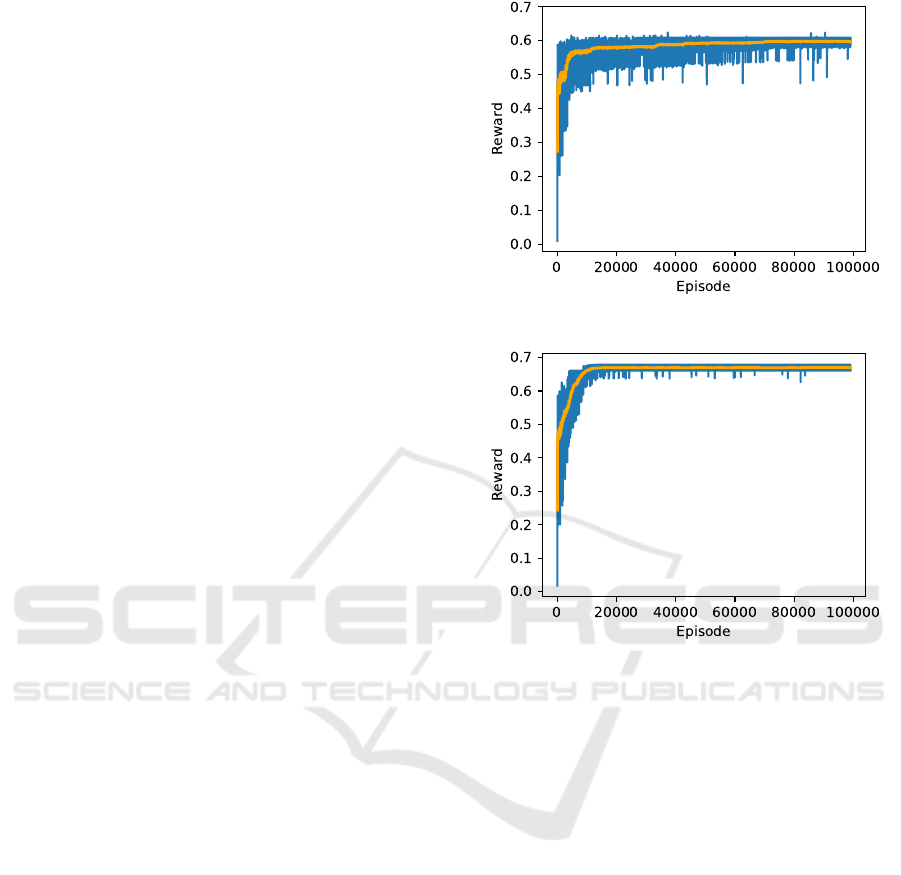
Figure 3: Discrete A2C.
Figure 4: Discrete PPO.
Overall, training the agents takes considerably
longer than the multi-discrete implementation. This is
a direct consequence of significantly longer episodes.
While the length of an episode in the multi-discrete
implementation will always be 1 step, the length of
the episode in the discrete implementation varies and
depends on the number of systems |S| within the IT
landscape that is being optimized. The training is fur-
ther complicated and, therefore, made longer when
the agent selects invalid actions for the problem, es-
pecially in the starting exploration stages where the
agent does not yet have a strong connection between
the number of placement options per system in the
observation and the action space figured out.
Furthermore, we observe that the A2C and PPO
agents, in general, require more episodes to achieve
consistent reward maximization. This is well observ-
able when the steady policy improvement and reward
increase observed and depicted in Figure 1 and Fig-
ure 2 for multi-discrete is compared to the discrete
training progress of the same algorithms, as depicted
in Figure 3 and Figure 4. Similarly to the case with
multi-discrete evaluation, A2C, on average, settles for
rewards that are 12.1% lower than that of PPO.
Figure 5: Discrete DQN.
Notably, DQN quickly learns to find higher-
quality results that produce higher rewards, but as
seen from Figure 5 the average reward achieved re-
duces as the episodes progress. In our case, this be-
havior is directly connected to the size of the replay
buffer. The default length of the replay buffer de-
picted in Figure 5 is 1 million steps. This has been
exhausted after just about 50 thousand episodes, so
some of the initial experiences collected from the ini-
tial steps are now being overwritten, which also di-
rectly influences the training of the underlying net-
work. Reducing the replay buffer further makes this
issue more prominent while increasing it allows the
agent to continue achieving higher average rewards
further. This illustrates the importance of the hyper-
parameter selection of the DRL agents.
5.3 Limitations
It is important to note that within this work, the focus
is on evaluating the overall viability of applying two
distinct types of action spaces to solve the IT land-
scape placement combination selection for enterprise
systems in a hybrid cloud environment. We do not at-
tempt to compare the selected algorithms against each
other. As such, we would require a more comprehen-
sive hyperparameter tuning of each to fit the discussed
optimization problem exactly, as a precise selection
of hyperparameters is shown (Liessner. et al., 2019;
Zhang et al., 2021) to significantly improve the per-
formance of DRL agents.
Hyperparameter optimization for machine learn-
ing, in general, can be complex, and this is espe-
cially the case with DRL due to the overall complexity
of the algorithms and the known to be computation-
ally expensive (Ying et al., 2024) training of under-
lying DNNs. This is a known challenge of working
with DNN-based solutions that even results in driv-
ing the development of specialized computer archi-
Deep Reinforcement Learning for Selecting the Optimal Hybrid Cloud Placement Combination of Standard Enterprise IT Applications
441

tectures (Jouppi et al., 2020), that are not available to
us in a required capacity at the time of writing this
work. Therefore, the exact fitting of the algorithms is
beyond the scope of this publication.
6 FUTURE WORK
In the next steps of our research, we plan to build
upon the concepts presented in this work and conduct
a comprehensive comparison of various DRL algo-
rithms, including those beyond the presented in this
work baseline DQN, A2C, and PPO. An important
part of this future step is the application of hyperpa-
rameter optimization approaches to DRL within the
application to enterprise IT landscape system place-
ment combination in a hybrid cloud.
For the purpose of the hyperparameter optimiza-
tion for DRL, we intend to rely on state-of-the-art
scalable solutions such as Ray Tune (Liaw et al.,
2018). Reliance on such a solution would facilitate
the time-efficient search of the best parameters for
each algorithm that might be considered for compari-
son, enabling making such a comparison in a realistic
time frame.
7 CONCLUSION
In this work, we proposed and evaluated two designs
for DRL environments that are meant to tackle the
challenge of optimizing the placement combination
for enterprise IT landscapes in a hybrid cloud envi-
ronment. The primary difference between the two dis-
cussed DRL environments is the design of the action
space. The problem can be approached with a multi-
discrete action space, where the entire placement so-
lution is generated at once, and the agent receives a
full reward. Alternatively, it can be tackled in a se-
quential manner with a discrete action space where
the DRL agent places one system at a time and strives
to maximize the reward at the end of the episode in-
stead of the immediate reward.
Both formulations of the DRL environment are
viable alternatives but with different sets of limi-
tations. Multi-discrete potentially allows for faster
training and execution but has scalability limitations
to problem definition sizes that exceed the initial ac-
tion space. The discrete action space requires a se-
quential execution of a number of steps that depend
on the size of the problem, which significantly in-
creases the length of training and effort before the fi-
nal placement decision is determined. Furthermore,
the multi-discrete variation of the environment has
potential limitations on the types of DRL algorithms
that can be applied to solve it.
REFERENCES
Aloysius, G. C., Bhatia, A., and Tiwari, K. (2023). Stabil-
ity and Availability Optimization of Distributed ERP
Systems During Cloud Migration. In Barolli, L., edi-
tor, Advanced Information Networking and Applica-
tions, pages 343–354, Cham. Springer International
Publishing.
Brockman, G., Cheung, V., Pettersson, L., Schneider, J.,
Schulman, J., Tang, J., and Zaremba, W. (2016). Ope-
nAI Gym.
Cecci, H. and Cappuccio, D. (2022). Workload Place-
ment in Hybrid IT - Making Great Decisions About
What, Where, When and Why. Technical Report
G00727702, Gartner Research.
Farshidi, S., Jansen, S., de Jong, R., and Brinkkemper, S.
(2018). A Decision Support System for Cloud Ser-
vice Provider Selection Problem in Software Produc-
ing Organizations. In 2018 IEEE 20th Conference on
Business Informatics (CBI), volume 01, pages 139–
148.
Frank, R., Schumacher, G., and Tamm, A. (2023). The
Cloud Transformation. In Frank, R., Schumacher, G.,
and Tamm, A., editors, Cloud Transformation : The
Public Cloud Is Changing Businesses, pages 203–245.
Springer Fachmedien, Wiesbaden.
Jin, Y., Wang, H., Chugh, T., Guo, D., and Miettinen, K.
(2019). Data-Driven Evolutionary Optimization: An
Overview and Case Studies. IEEE Transactions on
Evolutionary Computation, 23(3):442–458.
Jouppi, N. P., Yoon, D. H., Kurian, G., Li, S., Patil, N.,
Laudon, J., Young, C., and Patterson, D. (2020). A
domain-specific supercomputer for training deep neu-
ral networks. Commun. ACM, 63(7):67–78.
Jung, G., Mukherjee, T., Kunde, S., Kim, H., Sharma,
N., and Goetz, F. (2013). CloudAdvisor: A
recommendation-as-a-service platform for cloud con-
figuration and pricing. Proceedings - 2013 IEEE 9th
World Congress on Services, SERVICES 2013, pages
456–463.
Kaelbling, L. P., Littman, M. L., and Moore, A. W. (1996).
Reinforcement Learning: A Survey. Journal of Artifi-
cial Intelligence Research, 4:237–285.
Kharitonov, A., Nahhas, A., M
¨
uller, H., and Turowski, K.
(2023). Data driven meta-heuristic-assisted approach
for placement of standard IT enterprise systems in
hybrid-cloud. In Proceedings of the 13th International
Conference on Cloud Computing and Services Science
- CLOSER, pages 139–146. SciTePress / INSTICC.
Klar, M., Glatt, M., and Aurich, J. C. (2023). Per-
formance comparison of reinforcement learning and
metaheuristics for factory layout planning. CIRP
Journal of Manufacturing Science and Technology,
45:10–25.
Liaw, R., Liang, E., Nishihara, R., Moritz, P., Gonzalez,
J. E., and Stoica, I. (2018). Tune: A research platform
ICEIS 2025 - 27th International Conference on Enterprise Information Systems
442

for distributed model selection and training. arXiv
preprint arXiv:1807.05118.
Liessner., R., Schmitt., J., Dietermann., A., and B
¨
aker., B.
(2019). Hyperparameter optimization for deep re-
inforcement learning in vehicle energy management.
In Proceedings of the 11th International Conference
on Agents and Artificial Intelligence - Volume 2:
ICAART, pages 134–144. INSTICC, SciTePress.
Marquard, U. and G
¨
otz, C. (2008). SAP Standard Appli-
cation Benchmarks - IT Benchmarks with a Business
Focus. In Kounev, S., Gorton, I., and Sachs, K., ed-
itors, Performance Evaluation: Metrics, Models and
Benchmarks, pages 4–8, Berlin, Heidelberg. Springer.
Mazyavkina, N., Sviridov, S., Ivanov, S., and Burnaev, E.
(2021). Reinforcement learning for combinatorial op-
timization: A survey. Computers & Operations Re-
search, 134:105400.
Mell, P. and Grance, T. (2011). The NIST Definition of
Cloud Computing. Technical Report NIST Special
Publication (SP) 800-145, National Institute of Stan-
dards and Technology.
Mennes, R., Spinnewyn, B., Latre, S., and Botero, J. F.
(2016). GRECO: A Distributed Genetic Algorithm
for Reliable Application Placement in Hybrid Clouds.
Proceedings - 2016 5th IEEE International Confer-
ence on Cloud Networking, CloudNet 2016.
Mnih, V., Badia, A. P., Mirza, M., Graves, A., Lillicrap,
T. P., Harley, T., Silver, D., and Kavukcuoglu, K.
(2016). Asynchronous Methods for Deep Reinforce-
ment Learning.
Mnih, V., Kavukcuoglu, K., Silver, D., Rusu, A. A., Ve-
ness, J., Bellemare, M. G., Graves, A., Riedmiller,
M., Fidjeland, A. K., Ostrovski, G., Petersen, S.,
Beattie, C., Sadik, A., Antonoglou, I., King, H., Ku-
maran, D., Wierstra, D., Legg, S., and Hassabis, D.
(2015). Human-level control through deep reinforce-
ment learning. Nature, 518(7540):529–533.
M
¨
uller, H., Kharitonov, A., Nahhas, A., Bosse, S., and Tur-
owski, K. (2021). Addressing IT Capacity Manage-
ment Concerns Using Machine Learning Techniques.
SN Computer Science, 3(1):26.
Papadimitriou, C. H. and Tsitsiklis, J. N. (1987). The Com-
plexity of Markov Decision Processes. Mathematics
of Operations Research, 12(3):441–450.
Raffin, A., Hill, A., Gleave, A., Kanervisto, A., Ernestus,
M., and Dormann, N. (2021). Stable-Baselines3: Reli-
able Reinforcement Learning Implementations. Jour-
nal of Machine Learning Research, 22(268):1–8.
Sahu, P., Roy, S., and Gharote, M. (2024). CloudAdvisor
for Sustainable and Data Residency Compliant Data
Placement in Multi-Cloud. In 2024 16th International
Conference on COMmunication Systems & NETworkS
(COMSNETS), pages 285–287.
Sahu, P., Roy, S., Gharote, M., Mondal, S., and Lodha, S.
(2022). Cloud Storage and Processing Service Selec-
tion considering Tiered Pricing and Data Regulations.
In 2022 IEEE/ACM 15th International Conference on
Utility and Cloud Computing (UCC), pages 92–101.
Schulman, J., Wolski, F., Dhariwal, P., Radford, A., and
Klimov, O. (2017). Proximal Policy Optimization Al-
gorithms.
Sfondrini, N., Motta, G., and Longo, A. (2018). Public
Cloud Adoption in Multinational Companies: A Sur-
vey. In 2018 IEEE International Conference on Ser-
vices Computing (SCC), pages 177–184.
Shi, T., Ma, H., Chen, G., and Hartmann, S. (2020).
Location-Aware and Budget-Constrained Service De-
ployment for Composite Applications in Multi-Cloud
Environment. IEEE Transactions on Parallel and Dis-
tributed Systems, 31(8):1954–1969.
Sutton, R. S., McAllester, D., Singh, S., and Mansour,
Y. (1999). Policy Gradient Methods for Reinforce-
ment Learning with Function Approximation. In
Advances in Neural Information Processing Systems,
volume 12. MIT Press.
Tavakoli, A., Pardo, F., and Kormushev, P. (2018). Action
branching architectures for deep reinforcement learn-
ing. Proceedings of the AAAI Conference on Artificial
Intelligence, 32(1).
Towers, M., Kwiatkowski, A., Terry, J., Balis, J. U.,
De Cola, G., Deleu, T., Goul
˜
ao, M., Kallinteris, A.,
Krimmel, M., KG, A., Perez-Vicente, R., Pierr
´
e, A.,
Schulhoff, S., Tai, J. J., Tan, H., and Younis, O. G.
(2024). Gymnasium: A Standard Interface for Rein-
forcement Learning Environments.
Triantaphyllou, E. (2000). Multi-Criteria Decision Mak-
ing Methods. In Triantaphyllou, E., editor, Multi-
Criteria Decision Making Methods: A Comparative
Study, pages 5–21. Springer US, Boston, MA.
Venkatraman, A. and Arend, C. (2022). A Resilient, Ef-
ficient, and Adaptive Hybrid Cloud Fit for a Dy-
namic Digital Business. Technical Report IDC
#EUR149741222, International Data Corporation.
Wang, X., Wang, S., Liang, X., Zhao, D., Huang, J., Xu, X.,
Dai, B., and Miao, Q. (2024). Deep Reinforcement
Learning: A Survey. IEEE Transactions on Neural
Networks and Learning Systems, 35(4):5064–5078.
Watkins, C. J. C. H. and Dayan, P. (1992). Q-learning. Ma-
chine Learning, 8(3):279–292.
Weinman, J. (2016). Hybrid cloud economics. IEEE Cloud
Computing, 3(1):18–22.
Ying, H., Song, M., Tang, Y., Xiao, S., and Xiao, Z.
(2024). Enhancing deep neural network training ef-
ficiency and performance through linear prediction.
Scientific Reports, 14(1):15197.
Zhang, B., Rajan, R., Pineda, L., Lambert, N., Biedenkapp,
A., Chua, K., Hutter, F., and Calandra, R. (2021).
On the importance of hyperparameter optimization
for model-based reinforcement learning. In Baner-
jee, A. and Fukumizu, K., editors, Proceedings of
The 24th International Conference on Artificial Intel-
ligence and Statistics, volume 130 of Proceedings of
Machine Learning Research. PMLR.
Zhu, J., Wu, F., and Zhao, J. (2022). An Overview of
the Action Space for Deep Reinforcement Learning.
In Proceedings of the 2021 4th International Confer-
ence on Algorithms, Computing and Artificial Intelli-
gence, ACAI ’21, New York, NY, USA. Association
for Computing Machinery.
Deep Reinforcement Learning for Selecting the Optimal Hybrid Cloud Placement Combination of Standard Enterprise IT Applications
443