SQL vs NoSQL: Six Systems Compared

Martin

Corov

ak and Pavel Koupil

Department of Software Engineering, Charles University, Prague, Czech Republic

Keywords:

Database Management Systems, Performance, Benchmark, Static Analysis, Experimental Analysis.

Abstract:

The rise of Big Data has exposed the limitations of relational databases in handling large datasets, driving the

growth of NoSQL databases. Today, various database systems based on distinct models – or their combinations

– are available, raising the question of which is best suited for a speciﬁc use case. While several papers

compare subsets of these systems, they are often limited in scope. In this paper, we offer a comprehensive

comparison of six systems, representing all major data models, through both static and dynamic analysis. We

demonstrate their strengths and weaknesses across several realistic use cases.

1 INTRODUCTION

In the early 1970s, E. F. Codd’s relational data

model (Codd, 1970) became the standard for database

systems. However, the rapid advancements in tech-

nology and the growing need to manage massive data

volumes led to the development of new data models

and database management systems (DBMS). NoSQL

databases, introduced to address the limitations of tra-

ditional relational databases, have gained popularity,

particularly for handling the three Vs of big data: vol-

ume, velocity, and variety. These databases are de-

signed with scalability, availability, and performance

in mind, making them ideal for applications like so-

cial networks, IoT, and e-commerce, which demand

more than traditional relational DBMSs can offer.

Performance is crucial for any software sys-

tem, impacting user experience and competitiveness.

DBMS performance is often benchmarked by query

execution time, inﬂuenced by factors like hardware,

data model, and database design. While query perfor-

mance can be enhanced, it often comes at the cost of a

less expressive query language, leading to the devel-

opment of aggregate-oriented systems. These systems

optimize data retrieval by storing related data as sin-

gle units, so-called aggregates, thus improving per-

formance but increasing data redundancy. Since nei-

ther of these strategies is universally optimal, this pa-

per explores the conditions under which each should

be selected. The key contributions are as follows:

• We perform a static analysis of six popular

https://orcid.org/0000-0003-3332-3503

open-source systems (SQLite, MySQL, Neo4j,

ArangoDB, Cassandra, MongoDB), focusing on

their features and supported query languages.

• We compare the expressive power of the query

languages across different data models (i.e., rela-

tional, graph, column-family, and document).

• We design a range of common query scenarios

and dynamically compare the performance of the

selected systems.

• We provide recommendations for optimal query-

ing strategies based on the results of both the static

analysis and dynamic performance comparisons

across various data representations.

Outline The paper is organized as follows: Sec-

tion 2 reviews related work on querying and perfor-

mance benchmarking. Section 3 outlines the method-

ology. Section 4 focuses on the static analysis of fea-

tures and limitations of the selected DBMSs. Sec-

tion 5 compares the expressive power of query lan-

guages. Section 6 presents the dynamic analysis and

results of the experiments. In Section 7, we conclude.

2 RELATED WORK

We ﬁrst acknowledge the work of (Taipalus, 2024),

who systematically reviewed DBMS benchmarks,

highlighting common pitfalls in DBMS benchmark-

ing. Taipalus drew inspiration from (Raasveldt et al.,

2018), who proposed a fair DBMS performance test-

ing checklist, which we also followed in this paper.

Corov

cák, M. and Koupil, P.

SQL vs NoSQL: Six Systems Compared.

DOI: 10.5220/0013217300003928

Paper published under CC license (CC BY-NC-ND 4.0)

In Proceedings of the 20th International Conference on Evaluation of Novel Approaches to Software Engineering (ENASE 2025), pages 41-53

ISBN: 978-989-758-742-9; ISSN: 2184-4895

Database performance testing covers many

DBMSs with different data models, query languages,

and scalability levels. (Abramova and Bernardino,

2013) comparison of MongoDB and Cassandra

showed Cassandra’s superior performance. (Gy

odi

et al., 2015)’s work recommended MongoDB over

MySQL for data-intensive applications. (Wang

et al., 2015) showed that in-memory processing

with SQLite outperforms MySQL and MongoDB’s

disk-based processing. For highly connected

data, (Almabdy, 2018) found Neo4j better suited

than MySQL. (Sholichah et al., 2020) noted Neo4j’s

higher ﬂexibility but slower performance and greater

memory usage than MySQL.

Although the number of existing comparative

studies is not small, as we can see, they are usually

limited in scope. We aim to select a representative

set of DBMSs that covers all popular data models

and perform their extensive study. We will examine

both static features and query languages and perform

experimental measurements to objectively highlight

their strengths and weaknesses.

3 METHODOLOGY

To evaluate the selected DBMSs, we ﬁrst deﬁne

the selection criteria, focusing on data model sup-

port, open-source availability, single-node deploy-

ment, and popularity. We then detail the static anal-

ysis, where the capabilities and limitations of each

DBMS are assessed, followed by an examination of

the expressive power of their query languages. Fi-

nally, we present the dynamic analysis methodology,

including the queries executed, experimental conﬁg-

uration, and the process for evaluating query perfor-

mance across different systems, ensuring a compre-

hensive and fair comparison.

3.1 Selection Criteria

The selection of the database systems in this study

was guided by several key criteria. First, we pri-

oritized diversity in data model support, choosing

systems that represent relational, graph, document,

and wide-column models, allowing for a comprehen-

sive comparison of query performance across differ-

ent data structures. Second, we focused on databases

that are open-source, ensuring accessibility and trans-

parency in the implementation and testing processes.

Third, we required each system to have the ability to

deploy on a single computer node, making them suit-

able for environments with limited resources while

still providing insights into scalability and perfor-

mance. Finally, popularity was a signiﬁcant factor,

as we selected widely used systems with large user

and developer communities, as indicated by rankings

on DB-Engines

. This ensures the relevance to the

academic and industrial sectors.

3.2 Comparison Objectives

The objectives of the static analysis are to evaluate

the features of the selected DBMSs and their query

languages’ expressive power. The following system

features are reviewed:

• Data Model. The supported logical models, such

as relational, graph, document, and wide-column,

that determine how data is organized and struc-

tured.

• Data Types. The variety of basic/complex data

types, including collections, arrays, and user-

deﬁned types (UDTs).

• Consistency. Whether the system adheres to

ACID properties (ensuring strong consistency) or

BASE properties (offering eventual consistency

for scalability).

• Scalability. The system’s ability to scale horizon-

tally (by adding more nodes) or vertically (by up-

grading hardware resources).

• Sharding and Replication. The support for par-

titioning data across nodes (sharding) and main-

taining data redundancy through replication to en-

sure availability and fault tolerance.

• Schema Approach. The systems can be schema-

full, requiring a predeﬁned schema; schema-free,

allowing ﬂexible, on-the-ﬂy schema evolution; or

schema-mixed, which combines both approaches,

offering predeﬁned schema with some ﬂexibility.

• Entity and Relationship Representation. How en-

tities and relationships are modelled. Some sys-

tems explicitly support entities and relationships

(e.g., graph databases), while others focus only

on entities and use foreign keys or references to

represent relationships.

• Aggregates. Whether a system is aggregate-

ignorant or aggregate-oriented. The former sys-

tems use ﬂat structures and references between

entities, while the latter systems encapsulate com-

plex related data into a single document or ob-

ject, facilitating retrieval but possibly increasing

redundancy.

• Absence of Value Representation. How missing or

null values are handled. Some systems use NULL

https://db-engines.com/en/ranking

ENASE 2025 - 20th International Conference on Evaluation of Novel Approaches to Software Engineering

values, while others may leave missing properties

or combine both approaches.

For the expressive power of query languages,

we focus speciﬁcally on data manipulation language

(DML) operations, such as selecting, inserting, updat-

ing, and deleting data. We evaluate how each system’s

query language handles complex queries, including

joins, aggregations, traversals, and ﬁltering, empha-

sising efﬁciency and ﬂexibility. The aim is to deter-

mine whether certain systems are more suited to spe-

ciﬁc types of queries (or datasets).

3.3 Methodology of Dynamic Analysis

For the dynamic analysis, we selected an e-commerce

platform as the data domain, inspired by the

UniBench benchmark (Zhang and Lu, 2021). The

platform models products, vendors, customers, or-

ders, and social relationships. The data model in-

cludes both normalized (relational and graph models)

and denormalized (document and wide-column mod-

els) structures.

We selected a set of queries to cover various data

access patterns, including:

A. Selection, Projection, Source (of Data)

A1. Non-Indexed Columns: Select vendor named

‘Bauch - Denesik’.

A2. Non-Indexed Columns — Range Query:

Select people born between 1980-01-01 and

1990-12-31.

A3. Indexed Columns: Select vendor with the ID

24.

A4. Indexed Columns — Range Query: Select

people born between 1980-01-01 and 1990-12-

31.

B. Aggregation

B1. COUNT: Count the number of products per

brand.

B2. MAX: Find the most expensive product per

brand.

C. Joins

C1. Non-Indexed Columns: Join vendor and order

contacts on the type of contact.

C2. Indexed Columns: Join all products with their

orders.

C3. Complex Join 1: Retrieve all order details.

C4. Complex Join 2: Retrieve all people having

more than 1 friend.

C5. Neighborhood Search: Find all direct and

indirect relationships between people up to a

depth of 3.

C6. Shortest Path: Find the shortest path between

two people.

C7. Optional Traversal: Get a list of all people and

their friend count (0 if they have no friends).

D. Set Operations

D1. Union: Get a list of contacts (email and phone)

for both vendors and customers.

D2. Intersection: Find common tags between posts

and people.

D3. Difference: Find people who have not made

any orders.

E. Result Modiﬁcation

E1. Non-Indexed Columns Sorting: Sort prod-

ucts by brand.

E2. Indexed Columns Sorting: Sort products by

brand.

E3. Distinct: Find unique combinations of product

brands and the countries of the vendors selling

those products.

F. MapReduce:

F1. Find the number of orders per customer (only

those who have made at least 1 order).

The experiments were conducted on a virtual

machine with the following hardware conﬁguration:

Intel(R) Xeon(R) Gold 6348 CPU @ 2.60GHz (8

cores), 32 GB DDR4 RAM, and 80 GB SSD, running

Ubuntu 20.04 LTS. Docker and Docker Compose cre-

ated a consistent testing environment with Docker im-

ages for each DBMS, except for SQLite. We main-

tained default database conﬁgurations to ensure fair-

ness, adjusting settings only when necessary to sup-

port the testing process.

For each DBMS, the queries were translated into

the respective query language.

We ensured that

queries were consistent across systems to enable fair

comparisons. While each DBMS has unique features,

the goal was to retrieve equivalent data from each sys-

tem, with any format differences being adjusted dur-

ing result processing.

Query caching was disabled for all systems to

avoid skewed results. We also set a 300-second time-

out threshold for query execution. If a query exceeded

this limit, it was terminated.

Each query was executed 20 times to ensure reli-

able results. The minimum and maximum execution

times for each query were discarded, and the average

was calculated for the remaining values. The results

For reproduction purposes, all queries are avail-

able in the GitHub repository https://github.com/corovcam/

Query-Languages-Analysis-Thesis

SQL vs NoSQL: Six Systems Compared

were processed using a Jupyter notebook with Pan-

das

and NumPy

(see Section 6).

4 STATIC ANALYSIS – DATABASE

SYSTEMS

This section compares six popular database manage-

ment systems: SQLite, MySQL, Neo4j, ArangoDB,

Cassandra, and MongoDB. Each system is examined

based on key features, including consistency mod-

els, scalability, schema management, entity and re-

lationship types, and how they handle missing val-

ues. The accompanying table highlights the similar-

ities and differences between these systems. At the

same time, the following discussion explores unique

aspects of their architecture and functionality, offer-

ing deeper insights into their strengths and speciﬁc

use cases.

4.1 SQLite

SQLite (Contributors, 2024) is an open-source

RDBMS developed by Dwayne Richard Hipp. As of

March 2024, it ranks 10th on the DB-Engines list and

is widely used in web browsers, operating systems,

mobile devices, and embedded systems.

Unlike traditional databases, SQLite is server-less,

self-contained, and requires zero conﬁguration, mak-

ing it an ideal embedded database. It is lightweight,

around 250 kB, storing both data and schema in a sin-

gle ﬁle. Additionally, it can function as an in-memory

database

, where the entire database resides in mem-

ory for faster access. However, optimizing perfor-

mance can be more complex as data requirements in-

crease compared to systems like MySQL.

SQLite lacks built-in user management, access

control, or authentication. Instead, it relies on the host

operating system’s ﬁle permissions to control access.

Its unique feature is its ability to allow multiple appli-

cations to access the same database at the same time,

rare for server-less databases.

SQLite supports ﬁve core storage classes, such as

INTEGER and TEXT, with other common SQL types

like VARCHAR and DATETIME being handled through

Afﬁnity Types. As a ﬂexibly typed database, it allows

any type of data to be stored in any column, regard-

less of its declared type, which is an intentional design

https://pandas.pydata.org

https://numpy.org

https://sqlite.org/inmemorydb.html

https://www.sqlite.org/serverless.html

feature.

4.2 MySQL

MySQL (Corporation, 2024) is a widely used open-

source relational DBMS developed and maintained

by the Oracle Corporation. As of March 2024, it

ranks 2nd on the DB-Engines list, making it a pop-

ular choice for web applications and widely adopted

by high-proﬁle websites. Known for its strong perfor-

mance, reliability, and ease of use, MySQL is also

highly scalable, making it suitable for both small-

scale applications and large enterprise systems.

MySQL operates on a client-server architecture,

requiring a server to run. The server enables multi-

user access and provides essential features like access

control, user management, and built-in security. Due

to its extensive set of features, the initial setup can

be more complex than lightweight alternatives like

SQLite (see Section 4.1).

MySQL supports a range of data types, including

numeric, date/time, and various string types, along

with more advanced types like XML and JSON for

structured data. It also allows efﬁcient querying and

manipulation of JSON documents.

From version

8.0.17, it supports Multi-Valued indexes, enabling in-

dexing of JSON array values stored in columns.

4.3 Neo4j

Neo4j (Inc., 2024) is an open-source graph DBMS

developed by Neo4j, Inc., ranked 23rd on the DB-

Engines list (March 2024). It is commonly used in

areas requiring complex relationships between enti-

ties, such as social networks, recommender systems,

fraud detection, network analysis, and emerging ﬁelds

like ML, AI, and IoT.

Neo4j employs a labelled property graph (LPG)

model (Angles and Gutierrez, 2008), consisting of

nodes (vertices), relationships (edges), and key-value

pair properties. The model supports both basic graph

traversals (like depth-ﬁrst search) and complex algo-

rithms (e.g., shortest path or minimum spanning tree).

Neo4j operates on a client-server architecture,

communicating via HTTP or the high-performance

Bolt protocol. Though it was initially developed in

Java, it offers drivers for multiple programming lan-

guages.

Supported data types include simple types (e.g.,

https://www.sqlite.org/quirks.html

https://dev.mysql.com/doc/refman/8.0/en/json.html

https://dev.mysql.com/doc/refman/8.0/en/

create-index.html#create-index-multi-valued

ENASE 2025 - 20th International Conference on Evaluation of Novel Approaches to Software Engineering

strings, integers), structural types (lists, maps), tem-

poral (dates, durations), and spatial (points).

4.4 ArangoDB

ArangoDB (ArangoDB GmbH, 2024a) is an open-

source multi-model DBMS (MMDBMS) developed

by ArangoDB GmbH, ranked 84th on the DB-

Engines list (March 2024). Its ﬂexibility supports

various applications, including social networks, real-

time analytics, recommendation systems, and fraud

detection. Available both commercially and as a man-

aged cloud service via ArangoGraph Insights Plat-

form

As an MMDBMS (Lu and Holubov

a, 2019),

ArangoDB supports document, graph, and key-value

data models in a single core. It primarily works

with JSON-formatted data stored in a binary format

called VelocyPack

. Values can be primitive types

(e.g., boolean, string) or compound types (arrays, ob-

jects).

ArangoDB uses the RocksDB storage en-

gine (Zhang et al., 2016), a persistent key-value

store optimized for fast storage and retrieval of

large datasets. It supports concurrent writes with

document-level locks and ensures durability through

a write-ahead log.

4.5 Cassandra

Cassandra (The Apache Software Foundation, 2024)

is a wide-column DBMS, developed by Avinash Lak-

shman and Prashant Malik at Facebook (Lakshman

and Malik, 2010), and now maintained by the Apache

Software Foundation. As of March 2024, it ranks 12th

on the DB-Engines list. It is widely used in domains

needing high availability and fault tolerance, such as

event logging, messaging, e-commerce, and content

management systems, where fast reads and writes are

crucial.

Cassandra uses a wide-column model, organized

into column families (tables), which contain rows

(records) and columns (ﬁelds). Columns store key-

value pairs with timestamps, and rows are key-

linked collections of columns. Column families are

grouped into keyspaces (similar to databases), dis-

tributed across clusters using partitioners and repli-

https://arangodb.com/arangograph-insights-platform/

https://github.com/arangodb/velocypack

https://docs.arangodb.com/3.11/aql/fundamentals/

data-types/

https://docs.arangodb.com/3.11/components/

arangodb-server/storage-engine

cation strategies.

Cassandra draws on design concepts from Ama-

zon Dynamo

and Google Bigtable

, with a stor-

age engine based on the Log-Structured Merge-

Tree (Zhang et al., 2016), optimized for write-heavy

workloads.

Cassandra supports various types, including na-

tive types (strings, numbers), collections (lists, sets),

UDTs, and tuples. However, collection types may

cause performance issues due to full data scans, and

using sets is recommended over lists to avoid read-

before-write penalties.

4.6 MongoDB

MongoDB is a document-based DBMS developed by

MongoDB Inc., ranked 5th on the DB-Engines list

(March 2024). It is used for content management,

real-time analytics, and high-speed logging. Mon-

goDB is available as an open-source Community Edi-

tion, a commercial Enterprise Edition, or via the SaaS

solution MongoDB Atlas.

As a document-oriented DBMS, MongoDB stores

ﬂexible-schema JSON-based documents (ECMA In-

ternational, 2021). Internally, it uses BSON (Binary

JSON), which is more efﬁcient and allows documents

up to 16 MB in size.

Databases in MongoDB con-

sist of collections (similar to tables), grouping related

documents that are key-value pairs. Documents can

be nested, supporting complex data structures.

BSON supports standard JSON types (strings,

numbers, arrays) and additional types like datetime

and geospatial data in a binary format.

MongoDB uses the WiredTiger storage en-

gine, optimized for most workloads with features

like document-level concurrency, compression, and

checkpointing. The Enterprise version offers an in-

memory storage engine for speciﬁc use cases.

https://cassandra.apache.org/doc/4.1/cassandra/

architecture/overview.html

https://aws.amazon.com/dynamodb/

https://cloud.google.com/bigtable

https://cassandra.apache.org/doc/4.1/cassandra/

architecture/dynamo.html

https://cassandra.apache.org/doc/4.1/cassandra/cql/

types.html

https://www.mongodb.com/products

https://bsonspec.org/

https://www.mongodb.com/docs/manual/core/

storage-engines/

SQL vs NoSQL: Six Systems Compared

4.7 Comparison of Selected Systems

The comparison of DBMSs (see Table 1) reveals sev-

eral interesting distinctions that go beyond their ba-

sic features. One notable aspect is the ﬂexibility of-

fered by databases like ArangoDB and MongoDB,

which support both BASE and ACID models, allow-

ing them to adapt to different consistency and per-

formance needs. This dual approach offers a mid-

dle ground for developers requiring transactional in-

tegrity and performance in distributed environments.

Cassandra’s use of the BASE model, while fo-

cused on eventual consistency, offers tunable levels

of consistency, making it highly adaptable for high-

availability systems. Additionally, its lightweight

transaction model, powered by Paxos, allows it to

handle more consistent operations when necessary

without sacriﬁcing its distributed nature.

Neo4j stands out for its unique graph-based struc-

ture, where relationships between entities (edges) are

ﬁrst-class citizens. This suits it, particularly for ap-

plications like social networks and recommendation

systems, where interconnected data is key. The ﬂex-

ibility of relationships in Neo4j contrasts with rela-

tional DBMSs like MySQL and SQLite, which rely

on foreign keys to deﬁne associations.

Regarding scalability, Cassandra and MongoDB

lead the way with built-in horizontal scaling and

sharding capabilities, allowing them to handle mas-

sive datasets. While Neo4j is scalable in its Enter-

prise version, and ArangoDB also offers sharding, the

graph nature of Neo4j means scaling is more complex

than document-based system like MongoDB.

Another interesting detail is how Cassandra han-

dles relationships through data denormalization and

UDTs. While it lacks traditional foreign keys, its

approach is optimized for speed and partitioning,

making it highly efﬁcient in distributed environ-

ments despite requiring more manual data structur-

ing. Lastly, ArangoDB and MongoDB’s schema-

free nature, paired with optional schema validation,

strikes a balance between ﬂexibility and structure,

making them versatile choices for developers who

may need to evolve data models over time. This con-

trasts fully schema-based systems like MySQL and

SQLite, where schema changes can be more rigid.

In terms of absence handling, MongoDB and Cas-

sandra treat missing values distinctively, distinguish-

ing between null and missing properties, which is

a useful feature for more nuanced data management

compared to the simpler NULL handling in systems

like MySQL and SQLite.

5 STATIC ANALYSIS – QUERY

LANGUAGES

Next, this section studies and compares the expressive

power of query languages of the analysed DBMSs:

SQL, Cypher, AQL, CQL, and MQL. It explores

features like projection, selection, joins, and graph

traversal, highlighting how each language aligns with

its DBMS’s architecture and design goals.

5.1 Structured Query Language (SQL)

SQLite and MySQL employ SQL (Chamberlin and

Boyce, 1974) as its primary query language, a stan-

dard widely used in relational DBMSs. SQL is pow-

erful for data querying and manipulation, based on

the relational model (Codd, 1970) using relational al-

gebra and calculus (E. F. Codd, 1971).

It supports traditional CRUD operations and key

clauses like SELECT, FROM, and WHERE for data se-

lection and ﬁltering. Table joins, including JOIN

and OUTER JOIN, are crucial for handling rela-

tionships, and aggregation is performed via GROUP

BY and HAVING. Set operations such as UNION,

INTERSECTION, EXCEPT, and DISTINCT are also sup-

ported. Result modiﬁcations are handled by ORDER

BY, LIMIT, and OFFSET, while recursive queries use

WITH RECURSIVE.

While SQL can simulate MapReduce opera-

tions using GROUP BY ... HAVING, it is not designed

for distributed processing like Hadoop

. MySQL

follows the ANSI/ISO standards, including SQL-

2023 (ISO, 2023; Kelechava, 2018), and supports ad-

ditional features like Stored Procedures, Triggers, and

User-Deﬁned Functions, though there are minor devi-

ations (MySQL Corporation, 2024).

Similarly, SQLite adheres to ANSI/ISO standards

but omits some features

, such as clauses in ALTER

TABLE. It also imposes limits, like a maximum of 64

table joins per query

, affecting recursive queries.

5.2 Cypher

The main query language in Neo4j is Cypher, a

declarative, human-readable language designed for

pattern matching, allowing ﬂexible querying and ma-

nipulation of graph data without requiring a prede-

ﬁned schema. It supports all CRUD operations and

extends functionality with APOC (Awesome Proce-

dures on Cypher), which provides a vast collection

https://hadoop.apache.org/

https://sqlite.org/omitted.html

https://sqlite.org/limits.html

ENASE 2025 - 20th International Conference on Evaluation of Novel Approaches to Software Engineering

Table 1: Comparison of individual features of Database Management Systems (DBMS).

SQLite MySQL Neo4j ArangoDB Cassandra MongoDB

Data model Relational Relational Graph Multi-model Column Document

Consistency ACID ACID ACID BASE / ACID BASE BASE / ACID

Scalability V V / H V / H V / H V / H V / H

Sharding N Y

Y Y Y

Replication N Y Y Y Y Y

Schema Full Full Free Free Full Free

Entity types Relation Relation Vertex Document Table Document

Relations Foreign Key Foreign Key Edge Reference /

Embedded Doc;

Edges collection

Denormalization +

UDTs

Reference /

Embedded Doc

Aggregates Ignorant Ignorant Ignorant Oriented Oriented Oriented

Absence of value Null Null Absence Null Null / absence Null / absence

Query language SQL SQL Cypher AQL CQL MongoDB QL

MySQL NDB Cluster

Neo4j Enterprise

of additional procedures and functions.

Cypher’s DML features focus on the MATCH clause

to ﬁnd nodes and relationships, followed by a graph

speciﬁcation. The WHERE clause ﬁlters results, and

RETURN projects the selected paths, nodes, or prop-

erties. Additionally, OPTIONAL MATCH optionally

matches entities in the traversal.

Moreover, ORDER BY, SKIP, and LIMIT sort, skip,

and limit results, while WITH passes results be-

tween queries. Set operations can be performed us-

ing UNION, WHERE NOT (similar to SQL’s EXCEPT),

and the apoc.coll.intersection() function from

the APOC library. The CALL clause invokes user-

deﬁned/external functions, and FOREACH performs op-

erations on a list of items. Subqueries are supported

via CALL {MATCH ...}.

Cypher, by default, matches all nodes and rela-

tionships based on the graph speciﬁcation, with no

need for a MATCH * clause. Aggregation is tied to the

graph speciﬁcation itself rather than individual prop-

erties. Functions like collect() gather query re-

sults into a list, and other aggregation functions like

count(), min(), max(), avg(), and sum() allow for

result summarization.

5.3 Arango Query Language (AQL)

Arango Query Language (AQL), used in ArangoDB,

is a declarative query language capable of querying

multiple data models simultaneously, whether docu-

ments, graphs, or key-value pairs. It fully supports all

CRUD operations.

The core DML statement is FOR doc IN docs

RETURN doc, with RETURN {attr1:val1,...} al-

lowing document projection. Moreover, RETURN

DISTINCT ensures unique projections, and FILTER fa-

cilitates document selection using a set of logical op-

erators.

AQL excels in data aggregation through the

COLLECT ... INTO or WINDOW operation, enabling

grouping and sophisticated data summaries

. Ad-

ditionally, SORT, LIMIT offset, count, and LET

clauses handle sorting, limiting, and variable assign-

ment. AQL does not have speciﬁc set operations but

uses FILTER cleverly for similar results

Joins in AQL are simple to declare. A One-To-

Many join is achieved with nested FOR loops, while

Many-To-Many joins use embedded lists of document

IDs and subqueries. Furthermore, Edge Collections

model Many-To-Many relationships efﬁciently in the

graph model. Outer joins are achieved by ﬁltering

zero-length arrays

AQL supports graph traversals with the statement:

FOR vertex[, edge[, path]]

IN [min[..max]] INBOUND/OUTBOUND/ANY

startVertex GRAPH graphName

allowing unlimited traversals, subject to the max pa-

rameter of the query

5.4 Cassandra Query Language (CQL)

Apache Cassandra uses CQL as its query language,

closely resembling SQL, making it intuitive and easy

to learn. CQL supports features like CRUD opera-

tions, querying, and batch operations while focusing

on performance and scalability. It is also extensible,

allowing developers to add custom functions (UDF)

and data types (UDT).

https://docs.arangodb.com/stable/aql/

examples-and-query-patterns/grouping/#aggregation

https://docs.arangodb.com/stable/aql/

examples-and-query-patterns/difﬁng-two-documents/

https://docs.arangodb.com/stable/aql/

examples-and-query-patterns/joins/#outer-joins

https://docs.arangodb.com/3.11/aql/graphs/traversals

SQL vs NoSQL: Six Systems Compared

Cassandra’s DML operations use SQL-like

SELECT, FROM, and WHERE clauses with some key

differences

. Queries must begin by specifying

the partition key, followed by clustering columns.

Filtering on non-indexed columns is possible with

ALLOW FILTERING, but it’s discouraged due to un-

predictable performance impacts. Moreover, results

can be grouped using GROUP BY (only on primary key

values) and aggregated via standard or user-deﬁned

functions

. Ordering is restricted to clustering

columns, and limits can be applied using LIMIT and

PER PARTITION LIMIT.

A key characteristic of CQL is the lack of join sup-

port between tables. Therefore, Cassandra adopts a

query-driven architecture, requiring data to be denor-

malized and duplicated for complex queries, a trade-

off for its high availability and fault tolerance

Finally, Cassandra supports MapReduce for dis-

tributed processing through Hadoop integration, en-

abling big data processing across multiple nodes.

5.5 MongoDB Query API

MongoDB’s Query API (MQL) powers all CRUD and

aggregation operations, optimized for JSON (ECMA

International, 2021) and JavaScript (Mozilla Corpo-

ration, 2024), though it integrates with various lan-

guages like Java, Python, and C#. It is accessi-

ble via MongoDB Compass and the MongoDB Shell

(mongosh)

DML operations use the db.collection.find(

{att1:val1, att2:val2}) method to query docu-

ments based on criteria, supporting comparison, log-

ical, element, and other operators

. Sorting, limit-

ing, and skipping results can be done via .sort(),

.limit(), and .skip(), while .count() returns the

collection size, and .distinct() retrieves unique

ﬁeld values.

Complex aggregations are handled by

db.collection.aggregate() through an Ag-

gregation Pipeline composed of stages like $match

and $project for ﬁltering and projecting. Op-

erations like min, max, avg, sum, and count are

done in the $group stage, while set operations like

$unionWith, $setUnion, and $setIntersection

https://cassandra.apache.org/doc/4.1/cassandra/cql/

dml.html#select-statement

https://cassandra.apache.org/doc/4.1/cassandra/cql/

functions.html

https://cassandra.apache.org/doc/4.1/cassandra/

data modeling/data modeling rdbms.html

https://www.mongodb.com/docs/mongodb-shell/

https://www.mongodb.com/docs/manual/reference/

operator/query/

are supported.

The $lookup stage enables left outer joins be-

tween collections; $graphLookup handles recur-

sive graph queries or unlimited traversals

. These

lookups allow nesting queries by running addi-

tional pipelines on joined documents. Though

.mapReduce() is supported for distributed queries, it

is deprecated in favour of aggregation pipelines due

to better performance

5.6 Query Languages Comparison

Table 2 illustrates query language expressive power

differences across DBMSs, shaped by their data mod-

els and system architecture. As we can see, rela-

tional databases like MySQL and SQLite offer stan-

dard SQL features such as joins, unions, and recursive

queries, ideal for structured data but limited in han-

dling non-relational models like graphs or documents.

Neo4j’s Cypher, designed for graph traversal, enables

efﬁcient querying of highly connected data, providing

recursive queries and graph pattern matching that are

more user-friendly than relational systems.

Cassandra, built for distributed scalability, omits

joins and recursive queries. This reﬂects its high

availability and partition tolerance design, where

complex operations like joins would reduce efﬁ-

ciency. Consequently, data in Cassandra must be de-

normalized to handle relationships, prioritizing scala-

bility over query complexity.

MongoDB, with its document model, provides ro-

bust aggregation pipelines and ﬂexible schema ca-

pabilities, but its support for joins is through the

$lookup stage rather than native relational joins, re-

ﬂecting its JSON-oriented structure. ArangoDB, as a

multi-model database, supports rich features like joins

and graph traversals, offering more expressive query

capabilities across different data models, making it a

highly versatile option compared to other systems.

6 DYNAMIC ANALYSIS

Being acquainted with the features of the DBMSs,

this section presents the experimental results, includ-

ing the measured query statistics for the selected

DBMSs, visualized in Table 3. We provide insights

into the results and discuss which DBMS performs

best under different data access patterns. For each

query listed in 3.3, we summarize the results, identify

https://www.mongodb.com/docs/manual/reference/

operator/aggregation/lookup/

https://www.mongodb.com/docs/manual/core/

map-reduce/

ENASE 2025 - 20th International Conference on Evaluation of Novel Approaches to Software Engineering

Table 2: Data Manipulation Language features of particular DBMS(s).

SQLite (SQL) MySQL (SQL) Neo4j (Cypher) ArangoDB (AQL) Cassandra (CQL) MongoDB (MQL)

Projection SELECT SELECT RETURN RETURN

{attr1:val1,attr2:val2}

SELECT $project,

ﬁnd(attr1:val1,attr2:val2)

Source FROM FROM graph speciﬁcation FOR doc IN docs FROM db.[collection name]

Selection WHERE WHERE WHERE FILTER WHERE $match, ﬁnd()

Aggregation GROUP BY ...

HAVING

GROUP BY ...

HAVING

count, min, max, avg COLLECT ... INTO;

WINDOW

GROUP BY aggregation pipeline

Join JOIN JOIN - FOR a IN b

FOR c IN d

FILTER a.cId ==

c. id ...

- $lookup

Graph Traversal JOIN

JOIN MATCH FOR v IN IN-

BOUND/OUTBOUND

...

- $graphLookup

Unlimited Traversal WITH RECURSIVE WITH RECURSIVE

FOR v IN 0..MAX - - ($graphLookup$

with limitations)

Optional OUTER JOIN OUTER JOIN OPTIONAL MATCH “outer joins” - -

Union UNION UNION UNION

- $unionWith,

$setUnion

(aggregation)

Intersection INTERSECTION INTERSECTION apoc.coll.intersection

- $setIntersection

(aggregation)

Difference EXCEPT EXCEPT WHERE NOT

- $setDifference

(aggregation)

Sorting ORDER BY ORDER BY ORDER BY SORT ORDER BY sort

Skipping OFFSET OFFSET SKIP LIMIT offset, count - skip

Limitation LIMIT LIMIT LIMIT LIMIT LIMIT limit

Distinct DISTINCT DISTINCT DISTINCT RETURN DISTINCT DISTINCT db.docs.distinct( ... )

Aliasing AS AS AS LET doc = (...) AS ”alias” : ”$ﬁeld”

Nesting (SELECT ...) (SELECT ...) CALL {MATCH . . . } FOR d IN docs FOR

u IN d ...

- -

MapReduce - (GROUP BY ...

HAVING)

- (GROUP BY ...

HAVING)

- (COLLECT ...

INTO)

GROUP BY .mapReduce

;

aggregation pipeline

everything is matched by default with no limitation

everything is aggregated by default

deprecated

maximum of 64 tables

see (ArangoDB GmbH, 2024b)

the best and worst performing DBMS, and explore the

reasons behind their performance. Finally, we recom-

mend choosing the most suitable DBMS for speciﬁc

scenarios.

Non-Indexed Columns Selection (A1). Most

systems performed similarly when selecting non-

indexed columns, except for Apache Cassandra,

which required a full table scan using ALLOW

FILTERING. This makes Cassandra less ideal for non-

indexed selections unless the schema is well-deﬁned.

Non-Indexed Columns – Range Query (A2).

Cassandra outperformed other systems due to its op-

timization for range queries. However, using ALLOW

FILTERING could still cause performance issues with

large ranges. Cassandra’s performance in range

queries highlights its efﬁciency, especially when deal-

ing with large datasets.

Indexed Columns Selection (A3). All sys-

tems performed comparably when querying indexed

columns, as the ID was indexed in each system. Neo4j

was slightly slower, but the difference was minor.

When exact value queries rely on indexed columns,

all systems are generally effective, though schema de-

sign plays a crucial role.

Indexed Columns – Range Query (A4). Cas-

sandra excelled again in range queries involving in-

dexed columns, especially with larger datasets. How-

ever, for smaller datasets, performance across systems

was similar. This suggests Cassandra’s advantage in

range queries, particularly when dealing with exten-

sive data.

Aggregation COUNT (B1). Performance across

all systems was comparable, with Cassandra show-

ing slightly better results due to its optimization for

aggregation queries. Simple one-entity aggregations,

like counting, are efﬁciently handled by all systems,

with Cassandra’s slight edge making it a strong choice

for this pattern.

Aggregation MAX (B2). Similar to count, the

performance for ﬁnding the maximum value was con-

sistent across systems, with Cassandra again per-

forming slightly better. When aggregations are com-

bined with other operations like joins, other systems

may be more suitable depending on the speciﬁc use

SQL vs NoSQL: Six Systems Compared

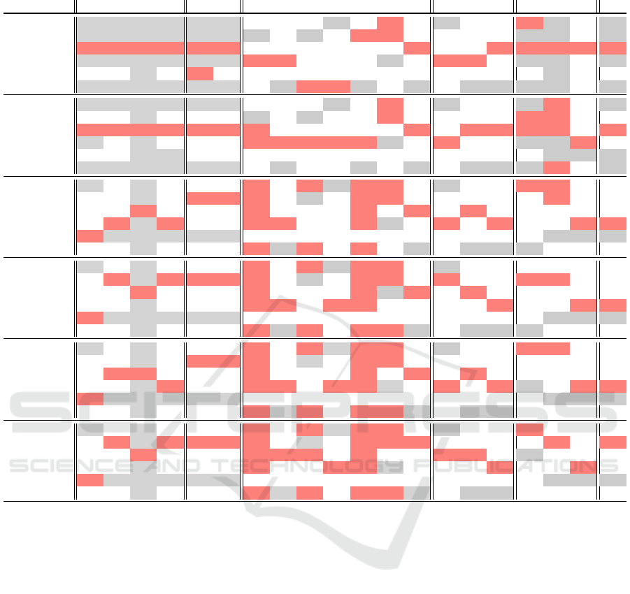
Table 3: Table illustrating the query execution times (the best in the category are grey, the worst are red).

Volume DBMS A1 A2 A3 A4 B1 B2 C1 C2 C3 C4 C5 C6 C7 D1 D2 D3 E1 E2 E3 F1

1k SQLite 0.00 0.00 0.00 0.00 0.00 0.00 4.34 0.01 0.70 0.00 5.76

†

0.01 0.02 0.01 0.00 0.01 0.00 0.01 0.00

MySQL 0.00 0.00 0.00 0.00 0.00 0.00 1.67 0.02 0.06 0.01 16.60

†

0.01 0.03 0.02 0.01 0.00 0.00 0.02 0.00

Neo4j 0.05 0.05 0.02 0.04 0.01 0.02 28.54 0.05 0.19 0.03 4.73 0.03 0.04 0.08 0.32 0.04 0.01 0.01 0.04 0.02

ArangoDB 0.00 0.00 0.00 0.00 0.00 0.00 45.69 0.07 0.19 0.05 15.33 0.00 0.02 0.09 0.08 0.01 0.00 0.00 0.03 0.00

Cassandra 0.01 0.01 0.00 0.01 0.01 0.01 0.00 0.00 0.01 0.00 n/a n/a 0.00 0.00 0.00 0.01 n/a 0.00 0.01 0.01

MongoDB 0.00 0.00 0.00 0.00 0.00 0.00 4.69 0.00 0.37 0.06 2.41 0.02 0.00 0.03 0.00 0.00 0.00 0.00 0.01 0.00

4k SQLite 0.00 0.00 0.00 0.00 0.00 0.00 43.99 0.04 6.77 0.02 39.95

†

0.02 0.05 0.04 0.01 0.01 0.01 0.03 0.00

MySQL 0.01 0.01 0.00 0.01 0.01 0.01 15.45 0.04 0.17 0.03 87.23

†

0.04 0.08 0.05 0.01 0.02 0.01 0.05 0.01

Neo4j 0.03 0.04 0.02 0.03 0.02 0.02

†

0.11 1.09 0.06 58.04 0.03 0.11 0.15 5.73 0.06 0.02 0.01 0.05 0.03

ArangoDB 0.00 0.01 0.00 0.01 0.01 0.01

†

0.20 1.12 0.28 144.54 0.00 0.04 0.28 0.42 0.04 0.01 0.00 0.14 0.01

Cassandra 0.02 0.01 0.00 0.00 0.01 0.01 n/a 0.00 0.00 0.00 n/a n/a 0.00 0.00 0.00 0.00 n/a 0.00 0.00 0.00

MongoDB 0.00 0.00 0.00 0.00 0.00 0.00 48.24 0.00 0.79 0.22 13.94 0.13 0.01 0.09 0.01 0.00 0.01 0.01 0.05 0.00

128k SQLite 0.02 0.05 0.00 0.07 0.12 0.13

†

1.85

†

0.43

† †

1.00 2.13 2.14 0.27 0.40 0.24 0.87 0.12

MySQL 0.07 0.14 0.00 0.14 0.20 0.21

†

2.16 9.97 0.93

† †

1.36 8.33 3.97 0.49 0.37 0.24 2.38 0.25

Neo4j 0.07 0.12 0.05 0.04 0.09 0.15

†

2.87 18.2 1.33

†

0.09 2.68 3.09

†

0.80 0.24 0.10 1.15 0.20

ArangoDB 0.03 0.15 0.00 0.15 0.15 0.19

†

6.31 20.67 8.07

†

0.07 0.89 8.56 10.38 1.21 0.29 0.10 3.63 0.35

Cassandra 0.32 0.01 0.00 0.00 0.00 0.01 n/a 0.00 0.01 0.00 n/a n/a 0.00 0.00 0.00 0.00 n/a 0.00 0.00 0.00

MongoDB 0.06 0.06 0.00 0.06 0.10 0.14

†

0.06

†

5.23

†

122.63 0.24 3.09 0.13 0.05 0.19 0.14 1.49 0.23

256k SQLite 0.04 0.11 0.00 0.15 0.22 0.24

†

4.00

†

0.83

† †

2.48 4.52 5.50 0.54 0.79 0.45 2.11 0.24

MySQL 0.15 0.31 0.00 0.31 0.46 0.47

†

5.62 25.02 2.13

† †

3.35 18.77 9.34 0.97 0.82 0.53 5.70 0.48

Neo4j 0.15 0.30 0.02 0.19 0.18 0.30

†

5.78 38.68 2.33

†

0.16 5.73 7.07

†

1.60 0.55 0.22 2.48 0.42

ArangoDB 0.07 0.29 0.00 0.26 0.22 0.33

†

13.61 40.86 16.41

†

0.19 1.70 15.78 22.00 2.22 0.46 0.15 8.33 0.75

Cassandra 0.78 0.01 0.00 0.01 0.01 0.01 n/a 0.00 0.01 0.00 n/a n/a 0.00 0.00 0.00 0.01 n/a 0.00 0.00 0.00

MongoDB 0.10 0.10 0.00 0.13 0.15 0.18 Err

0.07

†

10.80

†

Err

0.40 5.65 0.26 0.10 0.32 0.23 3.10 0.28

512k SQLite 0.06 0.21 0.00 0.32 0.47 0.51

†

7.99

†

1.54

† †

4.81 8.44 10.39 1.07 1.65 0.96 0.75 0.54

MySQL 0.27 0.52 0.00 0.50 0.80 0.83

†

6.35 23.60 3.14

† †

6.26 38.28 21.02 3.21 1.24 0.66 2.80 1.03

Neo4j 0.26 0.63 0.02 0.37 0.35 0.59

†

12.98 37.74 5.99

†

0.31 11.40 16.60

†

3.23 1.18 0.48 1.69 0.96

ArangoDB 0.14 0.58 0.00 0.51 0.52 0.60

†

32.92 53.16 33.48

†

0.27 3.13 36.08 45.78 4.85 1.02 0.30 10.41 1.67

Cassandra 1.85 0.01 0.00 0.00 0.01 0.01 n/a 0.00 0.01 0.00 n/a n/a 0.00 0.00 0.00 0.00 n/a 0.00 0.00 0.00

MongoDB 0.21 0.20 0.00 0.29 0.31 0.38 Err

0.16

†

21.54

† †

0.89 12.31 0.58 0.23 1.20 0.48 1.09 0.66

1024k SQLite 0.13 0.43 0.00 0.81 1.18 1.28

†

20.89

†

3.30

† †

10.13 20.26 22.23 2.32 3.26 1.96 1.80 1.69

MySQL 0.65 1.27 0.00 1.27 1.88 1.92

†

47.01 133.16 7.89

† †

51.89 111.85 44.02 10.28 3.23 2.02 7.82 6.91

Neo4j 0.41 0.69 0.30 0.71 0.69 1.17

† † †

14.12

†

0.61 24.93

† †

6.77 2.23 0.82 3.98 2.36

ArangoDB 0.27 0.91 0.00 1.17 0.96 1.16

†

78.06 146.85 69.19

†

0.50 6.35 87.44 95.39 11.50 2.40 0.59 12.38 4.52

Cassandra 3.60 0.01 0.00 0.00 0.01 0.01 n/a 0.00 0.01 0.00 n/a n/a 0.00 0.00 0.00 0.01 n/a 0.00 0.00 0.00

MongoDB 0.40 0.47 0.00 0.58 0.50 0.67 Err

0.30

†

44.29

†

Err

1.77 30.38 1.06 0.44 2.70 0.94 2.26 2.16

†

interrupted after 300 seconds

n/a

not available for efﬁcient execution

MongoServerError: Used too much memory for a single array

MongoServerError: $graphLookup reached maximum memory

consumption

case. Cassandra and MongoDB are particularly well-

suited for operations resembling MapReduce, espe-

cially when scalability is a key requirement.

Non-Indexed Columns Join (C1). Overall, no

system is a candidate to perform cross-product joins.

MySQL showed the best performance processing

cross-product joins (but only on small volumes),

while ArangoDB and Neo4j performed the worst,

struggling with cross-products even on very small

datasets. This query type is highly data-intensive,

making it unsuitable for systems like Cassandra,

which was dropped from testing due to the unman-

ageable data volume.

Indexed Columns Join (C2). Cassandra and

MongoDB performed best for indexed column joins,

excelling with denormalized schemas (i.e., query-

oriented design). Cassandra handled larger data vol-

umes better, while MongoDB was more efﬁcient with

smaller datasets, though both come with trade-offs

like increased disk space usage and costly updates.

Neo4j and ArangoDB performed worst, with Neo4j

struggling at higher data volumes due to timeouts.

While MySQL and SQLite offered reasonable per-

formance with smaller memory footprints, denormal-

ized schemas in Cassandra and MongoDB remain top

choices when disk space is not a concern.

Complex Join I (C3). Cassandra is the best for

complex joins (represented as redundant aggregates),

though its suitability depends on the use case (query-

oriented design vs data denormalization). Otherwise,

MySQL performed consistently well across all join

queries, offering a balanced option for more complex

joins when disk space is limited. SQLite struggled

with complex joins, and ArangoDB, while consistent,

lagged behind MySQL in performance.

Complex Join II (C4). The best performers were

Cassandra and SQLite, with SQLite handling one-

join queries better than MySQL (yet, SQLite demon-

ENASE 2025 - 20th International Conference on Evaluation of Novel Approaches to Software Engineering

strates limited scalability). ArangoDB performed the

worst, likely due to its multi-model approach. Cas-

sandra only counts friends, while MongoDB uses an

array with exact friend IDs, affecting performance.

Neighborhood Search (C5). Unexpectedly, no

system performed a query on more than 4k dataset.

On smaller datasets, the best performers were SQLite

and Neo4j. ArangoDB and MySQL performed worse.

MongoDB was not fully comparable due to incom-

plete result sets. Surprisingly, SQLite handled the

graph traversal well using recursive common table ex-

pressions but may struggle with larger joins. Neo4j

outperformed ArangoDB, making it the better graph

database for this query, but more research on its per-

formance is needed.

Shortest Path (C6). ArangoDB and Neo4j ex-

celled with optimized methods for ﬁnding the short-

est path. SQLite and MySQL performed poorly, espe-

cially at higher depths, struggling with graph traver-

sals. MongoDB’s breadth-ﬁrst search approach and

Cassandra’s lack of support for graph traversals made

them unsuitable for this comparison. Neo4j and

ArangoDB are the most effective for querying inter-

connected data, particularly in complex graph queries

like the shortest path.

Optional Traversal (C7). Cassandra and Mon-

goDB excelled, handling higher data volumes effec-

tively, while MySQL and Neo4j performed the worst.

ArangoDB outperformed Neo4j by a noticeable mar-

gin, suggesting it’s better suited for querying poten-

tially non-existent relationships. SQLite maintained

consistent performance across all data volumes. This

query highlights how systems differ in modelling and

processing data; Cassandra optimizes performance

by directly storing a friendCount property, reduc-

ing the need for additional tables, while SQLite and

ArangoDB may be more suitable for handling com-

plex or aggregate operations.

Union (D1). Cassandra and SQLite performed

best, with SQLite handling the normalized schema

surprisingly well. Neo4j struggled, experiencing

timeouts during testing. MySQL’s performance was

unexpectedly poor compared to SQLite, possibly

due to SQLite’s superior query optimizer for union

queries. ArangoDB’s performance was similar to

MySQL. MongoDB handled the query well, even

with an inter-collection join, though more research

is needed to assess the scalability of its $unionWith

operation. Depending on the frequency, SQLite is

ideal for infrequent unions, Cassandra for frequent,

and MongoDB for ﬂexibility.

Intersection (D2). Cassandra and MongoDB per-

formed best, particularly with lower data volumes.

Neo4j struggled with datasets of 4k or more, likely

due to the apoc.coll.intersection bottleneck.

SQLite again outperformed MySQL in this set opera-

tion. ArangoDB’s performance was better than Neo4j

but lagged behind relational databases. Cassandra and

MongoDB excel at real-time data processing for inter-

section queries, while SQLite offers an alternative for

minimizing server strain in such operations.

Difference (D3). Cassandra, MongoDB, and

SQLite performed best, while ArangoDB and

MySQL lagged. MySQL’s performance decreased

notably with the 1024k dataset, though the difference

was not drastic. For ﬁnding differences, Cassandra,

MongoDB, and SQLite are strong choices, with Cas-

sandra and MongoDB leveraging arrays or attributes

to reduce join operations, though this requires careful

handling of synchronization and denormalization.

Non-Indexed Columns Sorting (E1). All sys-

tems, except Cassandra, performed well in sorting by

non-indexed columns. Cassandra does not support

sorting by non-clustering columns.

Indexed Columns Sorting (E2). All systems per-

formed well in sorting by indexed columns, with Cas-

sandra showing a slight but almost unnoticeable per-

formance advantage.

Distinct (E3). Cassandra performed well in ﬁnd-

ing unique combinations of product brands and ven-

dor countries. ArangoDB was the worst performer.

Higher data volumes made it challenging to iden-

tify the slowest system, as reducing Vendor-Products

relationships caused execution time drops across all

systems. Cassandra is particularly efﬁcient, auto-

matically upserting duplicates using PRIMARY KEY.

SQLite may be a good choice for this query pattern

based on its strong performance in the experiments.

MapReduce (F1). Cassandra and MongoDB are

the top choices for very large datasets, thanks to their

scalability and support for horizontal operations.

While Cassandra performed well with smaller data

volumes, the results were inconclusive overall. This

query on small volumes resembles aggregation, with

similar execution times, but Cassandra’s lack of a

join operation and reliance on denormalized data

could limit its performance at larger scales. MySQL’s

performance notably degraded in larger datasets.

To sum up, our analysis shows that MySQL, SQLite,

and ArangoDB have the most expressive query lan-

guages, but Cassandra and MongoDB excel in per-

formance and scalability with large datasets. Neo4j

and ArangoDB are ideal for traversing interconnected

data, with ArangoDB offering more versatility in

data models and outperforming Neo4j in many cases,

though further research is needed to explore this fully.

Cassandra and MongoDB are the top performers

SQL vs NoSQL: Six Systems Compared

in speed and horizontal scalability, with Cassandra

being faster, while MongoDB is more feature-rich. As

data volumes increase, the choice depends on whether

joins and ﬂexibility or data redundancy and speed are

prioritized. SQLite handles a few joins efﬁciently,

while MySQL is better for complex joins. Cassan-

dra and MongoDB require more disk space and may

need additional application-layer processing, but their

speed is unmatched. For uncertain data structures or

query patterns, aggregate-ignorant systems are rec-

ommended. In contrast, aggregate-oriented systems

offer signiﬁcant speed advantages with more planning

and schema adaptation.

7 CONCLUSION

This paper presents an extensive comparative study

of various DBMSs employing distinct data manage-

ment strategies, including logical models, query lan-

guages, indexing techniques, and scalability. We con-

ducted both static and dynamic analyses to evaluate

the systems from multiple perspectives and address

common use cases. We conﬁrmed some of the expec-

tations, brought novel insights, and discovered unex-

pected behaviour.

We believe that the ﬁndings will assist users in se-

lecting the optimal solution for their needs, help ven-

dors identify areas for improvement, and provide re-

searchers with insights into open challenges and fu-

ture research opportunities.

ACKNOWLEDGEMENTS

This paper is based on thesis (

Corov

ak, 2024) and is

supported by the GA

CR project no. 23-07781S.

REFERENCES

Abramova, V. and Bernardino, J. (2013). NoSQL databases:

MongoDB vs cassandra. In Proceedings of the In-

ternational C* Conference on Computer Science and

Software Engineering, C3S2E ’13, page 14–22, New

York, NY, USA. ACM.

Almabdy, S. (2018). Comparative Analysis of Relational

and Graph Databases for Social Networks. In 2018 1st

International Conference on Computer Applications

& Information Security (ICCAIS), pages 1–4.

Angles, R. and Gutierrez, C. (2008). Survey of graph

database models. ACM Comput. Surv., 40(1).

ArangoDB GmbH (2024a). ArangoDB 3.11 Docs.

ArangoDB GmbH (2024b). Arangodb docs - difﬁng two

documents in AQL.

Chamberlin, D. D. and Boyce, R. F. (1974). SEQUEL:

A structured English query language. In SEQUEL:

A structured English query language, SIGFIDET ’74,

page 249–264, New York, NY, USA. ACM.

Codd, E. F. (1970). A relational model of data for large

shared data banks. Commun. ACM, 13(6):377–387.

Contributors, S. (2024). SQLite Documentation.

Corporation, M. (2024). MySQL 8.0 Reference Manual.

E. F. Codd (1971). A data base sublanguage founded on the

relational calculus. In Proceedings of the 1971 ACM

SIGFIDET (Now SIGMOD) Workshop on Data De-

scription, Access and Control, SIGFIDET ’71, page

35–68, New York, NY, USA. ACM.

ECMA International (2021). ECMA-404.

odi, C., Gy

odi, R., Pecherle, G., and Olah, A.

(2015). A comparative study: MongoDB vs. MySQL.

In 2015 13th International Conference on Engineer-

ing of Modern Electric Systems (EMES), pages 1–6.

Inc., N. (2024). Neo4j Documentation.

ISO (2023). ISO/IEC 9075-1:2023. [Online; accessed 11-

March-2024].

Kelechava, B. (2018). The SQL Standard - ISO/IEC

9075:2023 (ANSI X3.135) - ANSI Blog. The ANSI

Blog.

Lakshman, A. and Malik, P. (2010). Cassandra: a decentral-

ized structured storage system. SIGOPS Oper. Syst.

Rev., 44(2):35–40.

Lu, J. and Holubov

a, I. (2019). Multi-model Databases:

A New Journey to Handle the Variety of Data. ACM

Comput. Surv., 52(3).

Mozilla Corporation (2024). JavaScript – MDN.

MySQL Corporation (2024). MySQL :: MySQL 8.0 Refer-

ence Manual :: 1.6 MySQL Standards Compliance.

Raasveldt, M., Holanda, P., Gubner, T., and M

uhleisen,

H. (2018). Fair Benchmarking Considered Difﬁcult:

Common Pitfalls In Database Performance Testing.

In Proceedings of the Workshop on Testing Database

Systems. ACM.

Sholichah, R. J., Imrona, M., and Alamsyah, A. (2020). Per-

formance Analysis of Neo4j and MySQL Databases

using Public Policies Decision Making Data. In 2020

7th International Conference on Information Tech-

nology, Computer, and Electrical Engineering (ICI-

TACEE), pages 152–157.

Taipalus, T. (2024). Database management system perfor-

mance comparisons: A systematic literature review.

JSS, 208:111872.

The Apache Software Foundation (2024). Cassandra 4.1

Documentation.

Corov

ak, M. (2024). Experimental Analysis of Query Lan-

guages in Modern Database Systems. Bachelor thesis,

Charles University in Prague, Czech Republic.

Wang, Y., Zhong, G., Kun, L., Wang, L., Kai, H., Guo,

F., Liu, C., and Dong, X. (2015). The Performance

Survey of in Memory Database. In 2015 IEEE 21st

International Conference on Parallel and Distributed

Systems (ICPADS), pages 815–820.

ENASE 2025 - 20th International Conference on Evaluation of Novel Approaches to Software Engineering

Zhang, C. and Lu, J. (2021). Holistic Evaluation in Multi-

Model Databases Benchmarking. Distributed and

Parallel Databases, 39(1):1–33.

Zhang, W., Xu, Y., Li, Y., and Li, D. (2016). Improving

Write Performance of LSMT-Based Key-Value Store.

In 2016 IEEE 22nd International Conference on Par-

allel and Distributed Systems (ICPADS), pages 553–

560.

SQL vs NoSQL: Six Systems Compared