Predicting Socio-Demographic Characteristics from Load Proﬁles with

Varying Time Granularities

Dejan Radovanovic

1,2 a

, Maximilian Schirl

1 b

, Andreas Unterweger

1,2 c

and G

unther Eibl

1 d

Center for Secure Energy Informatics, Salzburg University of Applied Sciences, Puch bei Hallein, Salzburg, Austria

Paris Lodron University of Salzburg, Salzburg, Austria

Keywords:

Load Proﬁle Analysis, Supervised Machine Learning, Evaluation Methodology, Privacy.

Abstract:

Energy consumption data from smart meters has been shown to infer socio-demographic characteristics, which

impacts privacy. However, the impact of time granularity on the ability to classify such characteristics has not

yet been investigated in existing literature. In this paper, we answer this question by analyzing a dataset of

more than 1,000 households over one year. We obtain three main ﬁndings: (i) While a coarser time granularity

leads to decreased classiﬁcation performance, we ﬁnd that, unexpectedly, classiﬁcation performance only varies

insigniﬁcantly within two relatively large granularity intervals. For example, one-hour granularity exhibits

nearly the same classiﬁcation performance as 15-minute granularity. This indicates that, depending on the

use case, data collection can be minimized, as any resolution between 15 minutes and one hour can be used

without signiﬁcantly impacting prediction performance. (ii) We propose a new evaluation methodology where

an interpretable classiﬁcation algorithm can predict a household’s socio-demographic characteristics from a

load proﬁle of a single, arbitrary week of the year. Compared to existing methodologies, where training and

testing data are sampled from a single known week, using arbitrary weeks as input makes classiﬁcation harder,

thus requiring more sophisticated classiﬁcation algorithms. (iii) We present such an interpretable classiﬁcation

algorithm, which outperforms those that train and evaluate classiﬁers separately for each week. At the same

time, our algorithm exhibits a comparable performance to approaches that require a load proﬁle of the whole

year instead of a single, arbitrary week.

1 INTRODUCTION

Smart metering technology provides detailed energy

consumption data, offering valuable insights for utili-

ties and consumers to optimize energy usage, enable

dynamic pricing, and enhance efﬁciency (Darby, 2010;

Weranga et al., 2014). However, the widespread de-

ployment of smart meters raises privacy concerns due

to the detailed collection of electricity consumption

patterns, which can reveal sensitive information about

household habits, appliance use, and occupancy behav-

ior (Kim et al., 2011; Kolter and Jaakkola, 2012; Fan

et al., 2013). Since energy consumption is linked to

socio-demographic characteristics like dwelling type

and household income, load proﬁles can be exploited

to predict these characteristics (Beckel et al., 2013;

Beckel et al., 2014; Hopf et al., 2016; Wang et al.,

2019a). Increasing the time granularity of load proﬁles

https://orcid.org/0009-0000-6492-7620

https://orcid.org/0000-0003-0208-8088

https://orcid.org/0000-0002-3374-1636

https://orcid.org/0000-0001-9570-5246

has been suggested as a potential privacy enhancing

technology (Efthymiou and Kalogridis, 2010; Eibl and

Engel, 2015; Engel and Eibl, 2017; Erkin et al., 2013;

Finster and Baumgart, 2014). However, all of these

proposed methods primarily focus on ﬁne-grained load

proﬁles with short time intervals, such as milliseconds

or seconds, which are commonly utilized in Nonintru-

sive Load Monitoring (NILM) analyses (Hart, 1992;

Zoha et al., 2012).

In contrast, this paper investigates the privacy im-

plications of using coarse-grained load proﬁles with

time intervals ranging from minutes to days, aligned

with European Union recommendations that specify

a minimum resolution of 15 minutes for data collec-

tion (Commission, 2012). These recommendations

aim to strike a balance between data utility and privacy

preservation. On the one hand, ﬁner time granularity

offers a more informative and comprehensive view of

load patterns. On the other hand, such detailed data

poses a higher risk of identifying socio-demographics

and potentially infringing upon the privacy of indi-

viduals, as shown in (Lisovich et al., 2010; Molina-

Markham et al., 2010; Eibl and Engel, 2015).

Radovanovic, D., Schirl, M., Unterweger, A. and Eibl, G.

Predicting Socio-Demographic Characteristics from Load Proﬁles with Varying Time Granularities.

DOI: 10.5220/0013217400003953

Paper published under CC license (CC BY-NC-ND 4.0)

In Proceedings of the 14th International Conference on Smart Cities and Green ICT Systems (SMARTGREENS 2025), pages 87-98

ISBN: 978-989-758-751-1; ISSN: 2184-4968

This implies the main research question of this pa-

per: How does the time granularity of coarse-grained

load proﬁles inﬂuence the privacy of individual house-

holds with respect to the identiﬁcation of household-

speciﬁc socio-demographic characteristics? Prior re-

search has addressed facets of this question: (i) (Eibl

and Engel, 2015) analyzes the inﬂuence of time gran-

ularity on the inference of private information about

households; (ii) (Beckel et al., 2013; Beckel et al.,

2014; Hopf et al., 2016) focus on the identiﬁcation

of socio-demographic characteristics from 30-minute

load proﬁles.

Despite existing literature frequently highlighting

the need for further research, the speciﬁc impact of

time granularity on privacy, particularly for load pro-

ﬁles with intervals of 15 minutes or coarser in pre-

dicting socio-demographic characteristics, remains un-

derstudied (Alahakoon and Yu, 2016; Wang et al.,

2019b; Asghar et al., 2017). This paper addresses this

gap by examining the privacy inﬂuence of various

time granularities in weekly load proﬁles, from 15

minutes to 7 days, on the identiﬁcation of household-

speciﬁc socio-demographic characteristics. The study

is conducted using 1,589 suburban load proﬁles col-

lected over one year, offering new insights into how

time granularity affects privacy in the context of socio-

demographic prediction.

In contrast to existing methodologies that focus

on training and evaluating one speciﬁc week or use

an entire year’s data for prediction, our method tries

to predict socio-demographic characteristics from ar-

bitrary weeks of the year. This complexity requires

the classiﬁcation algorithm to take into consideration

various seasonal changes, intensifying the challenge

of the prediction task.

The paper is structured as follows: Section 2 ex-

plores relevant literature and Section 3 formally de-

ﬁnes the problem being addressed. Section 4 outlines

the methodology for predicting socio-demographic fea-

tures from weekly load proﬁles. Section 5 details our

ﬁndings, Section 6 compares them to existing methods

and discusses implications. Finally, Section 7 com-

pletes the study, highlighting conclusions and future

research.

2 RELATED WORK

Most existing research focuses on NILM, which disag-

gregates household consumption into individual appli-

ance loads using ﬁne-grained data with second-level

granularity (Zeifman and Roth, 2011; Zoha et al.,

2012; Armel et al., 2013; Pathak et al., 2018; Kim

et al., 2011; Kolter and Jaakkola, 2012; Fan et al.,

2013). While this approach provides detailed insights,

it also raises signiﬁcant privacy concerns, as ﬁne-

grained data can reveal sensitive information such as

appliance usage, occupancy patterns, and daily rou-

tines (Lisovich et al., 2010; Molina-Markham et al.,

2010; Greveler et al., 2012; Chicco, 2016; Eibl and En-

gel, 2015). Additionally, some studies have explored

the privacy risks related to detecting speciﬁc proper-

ties, such as appliance detection (Chen et al., 2013;

Kleiminger et al., 2013; Kleiminger et al., 2015).

In contrast, this work explores coarse-grained data

from several hundred households, with time intervals

of 15 minutes or coarser, a format aligned with Euro-

pean Commission guidelines for smart meters (Com-

mission, 2012). Prior research on coarse-grained pro-

ﬁles has largely focused on small datasets of 5-30

households, examining patterns such as daily consump-

tion, routines, and consumption forecasting using inter-

vals ranging from 15 minutes to one day (Verdu et al.,

2006; Silva et al., 2011; Abreu et al., 2012). Another

study explores the relationship between load proﬁles

and air temperature, analyzing hourly load proﬁles

from several hundred households (Birt et al., 2012).

Recent research has increasingly focused on pre-

dicting socio-demographic characteristics based on

household energy consumption behavior. (Beckel et al.,

2013) propose a classiﬁcation method that predicts

properties such as ﬂoor area and the number of occu-

pants from more than 3,000 Irish load proﬁles, col-

lected at 30-minute intervals over a period of 1.5 years.

Their supervised classiﬁcation system demonstrate

that most household properties could be accurately

predicted, achieving over 70 percent accuracy. In a

follow-up study, the authors extend their method by

incorporating regression techniques and enhancing fea-

ture extraction through the inclusion of temporal and

statistical characteristics of load proﬁles (Beckel et al.,

2014). Building on this work, (Hopf et al., 2016)

expand the feature set and further improve classiﬁca-

tion accuracy to 80 percent using the same dataset.

Meanwhile, (Viegas et al., 2016) develop a more inter-

pretable and transparent approach by leveraging fuzzy

models, achieving over 70 percent accuracy in pre-

dicting the presence of children, although predictions

for household income and education level were less

accurate, with around 60 percent accuracy. Building

on these advancements in predicting household char-

acteristics, other studies have focused on identifying

the presence of speciﬁc appliances within households.

For instance, (Burkhart et al., 2018) and (Ferner et al.,

2019). explored the detection of swimming pools us-

ing load proﬁles from the same geographic region,.

The ﬁrst major distinction of this work lies in the

methodological setting, speciﬁcally the training and

SMARTGREENS 2025 - 14th International Conference on Smart Cities and Green ICT Systems

evaluation process. Our approach builds on the feature

extraction technique proposed by (Beckel et al., 2014),

which utilized the Commission for Energy Regulation

(CER) dataset with a time granularity of 30 minutes

to classify socio-demographic characteristics such as

family home, large home, and house type. However,

there are two key differences between our work and

theirs: (i) While Beckel et al. primarily focused on as-

sessing data utility our focus shifts towards assessing

privacy preservation achieved through varying time

granularities. (ii) There is also a signiﬁcant divergence

in the training methodology. Beckel et al. trained and

evaluated their model using data from the same week

(week 26). In contrast, we train our model using a

full year of data, organized into weekly snippets, and

then test it by predicting socio-demographic charac-

teristics for a single, arbitrary, and unknown week.

This introduces more variability and complexity, as

our model needs to account for seasonal ﬂuctuations

and other temporal changes. While this approach pro-

vides more training data (52 weeks per household), it

also brings uncertainty in predicting characteristics for

an unknown week. By incorporating weeks from all

seasons, our goal is to improve the model’s ability to

generalize to any given week, regardless of seasonal

consumption variations. It turns out that our approach

leads to better performance values as described in more

detail in Section 6.

The second distinguishing factor is the evaluation

of how time granularity impacts the prediction perfor-

mance of socio-demographic information. Investiga-

tions into the inﬂuence of varying time granularities

are relatively scarce and predominantly focus on ﬁne-

grained load proﬁles. For instance, (Huchtkoetter and

Reinhardt, 2020) demonstrated that temporal granu-

larity signiﬁcantly impacts the accuracy of load disag-

gregation in the context of NILM, with the coarsest

resolution considered being 5 minutes. Similarly, (Her-

nandez et al., 2020) examined the importance of se-

lecting the appropriate temporal resolution for char-

acterizing household load proﬁle features, using data

from four Spanish households. Their ﬁndings suggest

that high-resolution load proﬁles, with a granularity

of 0.5 seconds, are effective in capturing consumption

ﬂuctuations across households. (Granell et al., 2015)

investigated the effect of temporal resolution on clus-

tering techniques applied to ﬁne-grained data, using

an acquisition rate of 7-8 seconds from Bulgarian and

English households in 2010. Their study concluded

that granularity levels between 4 and 60 minutes yield

optimal clustering performance, with a notable decline

in effectiveness observed beyond 60 minutes.

The most related work in this area studies the im-

plications of time granularity on edge detection meth-

ods (Eibl and Engel, 2015). The investigation high-

lights that a decrease in the appliance use detection rate

occurs when the time interval between measurements

surpasses half of an appliance’s on-time. Additionally,

the authors demonstrate that an overall decrease in the

measurement time interval, indicating coarser granular-

ity, leads to weaker detection results. (Engel and Eibl,

2017) introduce an privacy-preserving approach for

non-intrusive load monitoring that exploits the privacy-

preserving property of decreasing time granularities

which was found in (Eibl and Engel, 2015). Load

data is transformed into multiple resolutions, and each

resolution is encrypted, ensuring end-to-end security

and access control. Additionally, the study examines

this multi-resolution method’s compatibility with other

privacy-enhancing technologies, offering greater ﬂexi-

bility in preserving privacy.

Summarizing, this paper differs from most litera-

ture in two aspects: (i) the analysis of coarse-grained

electricity consumption proﬁles, with intervals ranging

from 15 minutes to 7 days from a large dataset with

1,589 households are examined and (ii) it is studied

how data-granularity inﬂuences the identiﬁcation of

household-speciﬁc socio-demographic characteristics.

3 PROBLEM DEFINITION

In an attack scenario where a set of households’ elec-

tricity consumption data alongside matching socio-

demographic information is leaked or made publicly

available (e.g., the datasets used in (Beckel et al., 2013;

Beckel et al., 2014; Burkhart et al., 2018; Ferner et al.,

2019; Radovanovic et al., 2022)), an attacker has ac-

cess to weekly load proﬁles

for a set of households

and their corresponding socio-demographic char-

acteristics. Consumption is measured in a speciﬁc

time granularities

∆t

. The goal of the attacker is to

generate a classiﬁer

∆t

that can predict a binarized

household-speciﬁc socio-demographic characteristic

(label)

from the available load proﬁles. The adver-

sary uses this classiﬁer

∆t

to determine the label

for an unknown household given a weekly energy con-

sumption snippet

˜w,∆t

of an arbitrary week

˜w

of the

year. Formally, the classiﬁer is a function

∆t

: R

→ {0, 1}: c

˜w,∆t

7→ y (1)

Consequently, this classiﬁer may then be ap-

plied to weekly load proﬁles without matching socio-

demographic characteristics available, posing poten-

tial privacy concerns. The number of values

the weekly consumption snippet decreases when time

granularity ∆t gets coarser.

Predicting Socio-Demographic Characteristics from Load Proﬁles with Varying Time Granularities

2. Decrease Resolution 3. Feature Extraction

4. Classification

5. Evaluation

1. Preparing Weekly Snippets

family_home

large_home

sauna

...

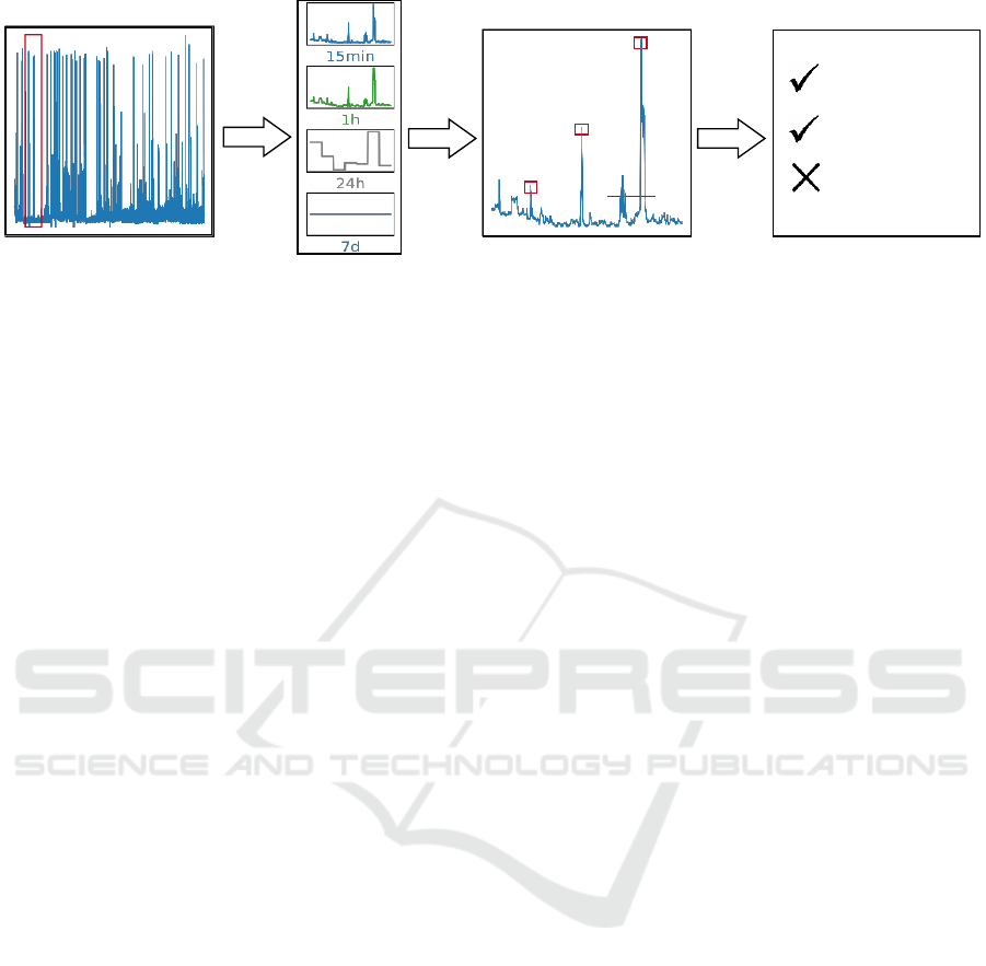
Figure 1: Methodological overview consisting of 5 steps: 1. preparing weekly snippets, 2. decrease of temporal resolution, 3.

feature extraction, 4. classiﬁcation, 5. evaluation.

The goal of this paper is to study the inﬂuence

of the time granularity

∆t

on the classiﬁcation perfor-

mance. The expectation is that, similar to existing

literature, the classiﬁer

∆t

gets worse as the time gran-

ularity ∆t is increased.

4 EXPERIMENTAL SETUP &

METHODOLOGY

Supervised machine learning techniques are employed

to assess how different time granularities of load pro-

ﬁles impact the prediction of household-speciﬁc socio-

demographic characteristics. The methodology, illus-

trated in Figure 1, consists of ﬁve stages: preparing

weekly snippets, decrease of temporal resolution, fea-

ture extraction, classiﬁcation, and evaluation. Details

on the selection of household-speciﬁc characteristics

and the data preparation are provided in Sections 4.2

and 4.3. Next, Section 4.4 addresses reducing the time

granularity of load proﬁles, followed by feature ex-

traction (Section 4.5), classiﬁcation (Section 4.6), and

evaluation (Section 4.7).

Before providing a step-by-step description of

the methodology, Section 4.1 offers an overview

of the dataset, which includes 15-minute load pro-

ﬁles collected over a year and their associated socio-

demographic characteristics.

4.1 Dataset

The used dataset, PEAK Load Data, stems from a

ﬁeld test, which collected electricity consumption pro-

ﬁles of 1,589 suburban households in Upper Austria

via smart meters between September 30, 2017 and

October 15, 2018. The ﬁeld test aimed at testing var-

ious incentive schemes for motivating consumers to

shift loads towards times of high renewable production.

More information about the study and the collection

of the data can be found in (Radovanovic et al., 2022).

The acquired data contains accumulated 15-

minute load proﬁles and household-speciﬁc socio-

demographic characteristics e.g., household type,

household size, household appliances and heating type.

To put some of the suburban household characteristics

into perspective, the following statistics are illustrated:

The yearly average energy consumption per household

is 5,327 kWh, with the median being 4,409 kWh and a

standard deviation of 3,721 kWh. The average house-

hold size is 138 (mean), 130 (median) and 58 (standard

deviation) in square meters, respectively. With 2.8 and

1.2 residents per household, respectively.

4.2 Selection of Household-Speciﬁc

Characteristics & Class Labels

Table 1 shows some characteristics gathered during the

ﬁeld test and their absolute frequencies, indicating the

number of positive and negative samples for each char-

acteristic. The selection of certain characteristics for

the prediction task is inﬂuenced by three main criteria:

First, their potential impact on privacy, with aspects

like household composition (e.g., family, single) iden-

tiﬁed as more sensitive compared to factors such as

heating type, as highlighted in (Beckel et al., 2012).

Second, we align our choice with characteristics used

in (Beckel et al., 2014) to maintain comparability with

existing classiﬁcation results. Third, the imbalance

ratio of the characteristics is also considered, with a

threshold of ﬁve being chosen to ensure a balanced dis-

tribution of positive and negative samples, addressing

the data imbalance issue discussed in more detail in

Section 4.6. This approach enables a balanced analy-

sis of the bold characteristics, emphasizing enhanced

privacy considerations.

Preceding the utilization of these characteristics, la-

bel binarization is applied to multi-class or numerical

data for clarity. For instance, households are labeled as

SMARTGREENS 2025 - 14th International Conference on Smart Cities and Green ICT Systems

family home if they have more than two residents, and

as large home if the living area exceeds 100 square me-

ters (Beckel et al., 2014). This labeling is consistently

applied across the dataset, with socio-demographic

details repeated for all 52 weekly data snippets in the

classiﬁcation task.

Table 1: List of household-speciﬁc characteristics and their

number of positive and negative samples, respectively.

Characteristic

Number

Positives

Number

Negatives

Imbalance

Ratio

family home 595 613 1.03

dryer 713 495 1.44

heat pump 400 808 2.02

split house 829 379 2.19

large home 831 377 2.20

deep freezer 868 340 2.55

pool 328 880 2.68

apartment 283 925 3.27

gas heating 280 928 3.31

electric water 274 931 3.40

sauna 256 952 3.72

home owned 967 241 4.01

4.3 Preparing Weekly Snippets

The preprocessing steps included: (i) removing house-

holds with excessive missing data, (ii) grouping load

proﬁles into weekly snippets, and (iii) selecting and bi-

narizing labels for classiﬁcation. The original dataset

comprises 1,589 households, but due to missing data

from issues like meter disruptions or changes, the num-

ber of usable households is reduced to 1,208. Only

data from a common period of 52 full weeks (Octo-

ber 2, 2017, to September 29, 2018) is used to ensure

seasonal coverage and comparability. Each house-

hold’s yearly load proﬁle is then regrouped into 52

weekly snippets (Beckel et al., 2014; Radovanovic

et al., 2022). With the original 15-minute time gran-

ularity, this results in a data matrix of size

n ×m

with

n = 1, 208·52 = 62, 816

and

m = 7 ·24 ·4 = 672

where

describes the number of household-week com-

binations and

represents the number of consumption

measurements for these weekly load proﬁles.

4.4 Decrease of Temporal Resolution

Prior to analyzing the privacy inﬂuence of differ-

ent time granularities, it is necessary to generate

load proﬁles with coarser granularity. The prepro-

cessed data with 15-minute intervals, shaped as

n ×m

(

1, 208 ·52 ×7 ·24 ·4

), is used as input. Aggregation is

performed by summing the consumption values within

each time interval. For instance, increasing the granu-

larity from 15 minutes to 30 minutes involves summing

the two measurements in that interval. This process

changes the shape of the data matrix, reducing the

number of measurements,

, based on the new time in-

terval

∆t

. For a 30-minute granularity (

∆t

), the matrix

has

m = 336

(

7·24·2

) data points, halving the original

value of

. This procedure is applied for all resolu-

tions in Figure 3, generating a separate data matrix

with n = 1, 208 ·52 and varying m for each ∆t.

4.5 Feature Extraction

Feature extraction, essential for classiﬁcation, trans-

forms preprocessed data into a more efﬁcient for-

mat (Bishop, 2006), generating load-proﬁle-speciﬁc

features for each household across all time granular-

ities (

∆t

) and household-week combinations. Three

initial approaches are explored: automated extraction

using the ts-fresh

library, autoencoder-based encod-

ing, and manual feature crafting. The handcrafted

approach was prioritized for its ability to simplify the

feature space and enhance interpretability, and align

with previous work, speciﬁcally adapting features from

Beckel et al. (Beckel et al., 2012; Beckel et al., 2013;

Beckel et al., 2014) for comparability.

Table 2 lists 35 off-the-shelf numerical charac-

teristics, consisting of ﬁve categories: (i) consumption

characteristics, (ii) ratios of consumption characteris-

tics, (iii) temporal dynamics, (iv) statistical properties,

and (v) the ﬁrst ten principal components. These fea-

tures span from daily consumption aggregates and

comparative ratios between different times, to event-

speciﬁc markers and statistics, including variance and

the frequency of peaks. The focus on event-speciﬁc

markers and statistical features, especially those high-

lighted in bold, illustrates their heightened sensitivity

to load proﬁles at ﬁner, 15-minute intervals. This dis-

tinction underscores the greater depth and detail in

analyzing consumption patterns at these ﬁner granu-

larities, compared to the broader, more generalized

insights derived from coarser, hourly data. For in-

stance, a water cooker’s peak energy consumption is

detectable at 15-minute granularity but remains invisi-

ble at one-hour granularity.

Most statistical methods for computing load-

proﬁle-speciﬁc features assume a normal distribu-

tion (Osborne, 2002; Beckel et al., 2014). To align

with this assumption, we apply the same transforma-

tion functions as in (Beckel et al., 2014). Features

that could result in undeﬁned expressions, such as

dividing zero by zero, are replaced with zero. For in-

stance, when only a single electricity consumption is

https://tsfresh.readthedocs.io

Predicting Socio-Demographic Characteristics from Load Proﬁles with Varying Time Granularities

Table 2: List of features that are used for the classiﬁcation, initially proposed by Beckel et. al (Beckel et al., 2014). Except for

the ﬁrst two features, c total and c weekend, all of the listed features are computed only over the 5 working days (Monday to

Friday). The last column shows the maximum resolution up to which the corresponding feature is computable.

Feature Category Feature Description

Max.

Resolution

(1) Consumption

c total

Total consumption of one week including the

weekend

7 days

c weekend

Total consumption of the weekend Saturday and

Sunday

2 days

c workday

Total consumption of the 5 workdays Monday to

Friday

5 days

c daytime

Total consumption during daytime (6 a.m. - 10

p.m.)

4 hours

c morning

Total consumption of mornings (6 a.m. - 10 a.m.)

4 hours

c noon

Total consumption around noon (10 a.m. - 2 p.m.)

4 hours

c evening

Total consumption in evening time (6 p.m. - 10

p.m.)

4 hours

c night

Total consumption during night time (1 a.m. - 5

a.m.)

4 hours

c max Maximum consumption value at workdays 5 days

c min Minimal consumption value at workdays 5 days

(2) Ratios

r mean/max

Mean consumption divided by maximum con-

sumption

5 days

r min/mean

Minimum consumption divided by mean con-

sumption

5 days

r morning/noon

Morning consumption divided by consumption

around noon

4 hours

r evening/noon

Evening consumption divided by consumption

around noon

4 hours

r noon/day

Consumption around noon divided by daytime

consumption

4 hours

r night/day

Night consumption divided by daytime consump-

tion

4 hours

r workday/weekend

Workday consumption divided by weekend con-

sumption

2 hours

(3) Temporal

t above 0.5kw

Proportion of time, where consumption ex-

ceeds 0.5 kW

5 days

t above 1kw

Proportion of time, where consumption ex-

ceeds 1 kW

5 days

t above 2kw

Proportion of time, where consumption ex-

ceeds 2 kW

5 days

t above mean

Proportion of time, where consumption ex-

ceeds the mean

5 days

(4) Statistical

s variance Variance of all weekly consumption values 3 days

s diff Sum of changes compared to previous days 3 days

s x-corr Cross-correlation of subsequent days 12 hours

s number peaks Number of peaks over the week 3 days

(5) PCA Components

PCA

First principal component 5 days

PCA

, . . . ,PCA

Principal components 2 to 10 12 hours

recorded per day, ratios like evening/noon consump-

tion (r evening/noon) cannot be calculated. Table 2

lists the maximum resolution up to which all 35 fea-

tures can still be computed.

SMARTGREENS 2025 - 14th International Conference on Smart Cities and Green ICT Systems

4.6 Classiﬁcation

Supervised machine learning techniques are used to

classify house- hold-speciﬁc socio-demographic char-

acteristics. This involves training a model to differenti-

ate between two classes (positive and negative) based

on extracted features from the training data. Essen-

tially, the classiﬁer learns the relationship between an

input feature vector and the corresponding class label.

For training and evaluation, a subset of known class

labels (Table 1) and their associated feature vectors

(Table 2) is computed.

A signiﬁcant challenge when working with ﬁeld

test data, such as the dataset described in Section 4.1,

is the class imbalance for certain characteristics, as

shown in Table 1. For instance, there are 256 house-

holds with a sauna and 952 without. Classiﬁers trained

on such imbalanced labels may exhibit bias, incor-

rectly assigning samples from the minority class to the

majority class. Previous studies have demonstrated

that this class imbalance negatively affect the per-

formance of certain classiﬁers (Beckel et al., 2013;

Beckel et al., 2014).

To mitigate this issue, data undersampling is ap-

plied during training, a common method for handling

class imbalances (Japkowicz, 2000; He and Garcia,

2009). In this approach, random samples from the

overrepresented class are removed to ensure that both

positive and negative classes are equally represented,

with the sample size adjusted to match that of the un-

derrepresented class. Importantly, this undersampling

is only applied to the training and validation sets, leav-

ing the test set unaffected for proper evaluation.

Numerous classiﬁers suitable for binary clas-

siﬁcation tasks are well-documented in the litera-

ture (Bishop, 2006), differing in their implementation

and computational complexity. In this study, three

classiﬁers have been selected: (i) the

XGBoost

classi-

ﬁer (Chen and Guestrin, 2016), (ii) the support vector

machine (

SVM

) (Hearst et al., 1998) and (iii) a simple

version of a neural network, the multi layer perceptron

(

MLP

) (Haykin, 1998). These classiﬁers are used as

off-the-shelf algorithms and are applied without in-

depth parameter-optimization.

XGBoost

is chosen as

the primary classiﬁcation method to enable a detailed

analysis of feature importance and relationships.

4.7 Evaluation Measures

In the domain of supervised machine learning, the

accuracy, deﬁned as the ratio of the number of cor-

rect classiﬁcations to the total number of samples, is a

commonly used metric for evaluating classiﬁer perfor-

mance (Sokolova and Lapalme, 2009). The accuracy

can be calculated as follows:

ACC =

T P + T N

T P + T N + FP + FN

. (2)

TP, FN, FP, and TN represent the number of sam-

ples that are correctly predicted as positive, incorrectly

predicted as negative, incorrectly predicted as posi-

tive, and correctly predicted as negative, respectively.

Precision and recall are calculated as follows:

Precision =

T P

T P + FP

, Recall =

T P

T P + FN

(3)

Thus, the F

score is deﬁned as:

= 2 ·

Precision · Recall

Precision + Recall

. (4)

Accuracy and

score are commonly used statistics

that represent the proportion of correct predictions and

the harmonic mean of precision and recall, respectively.

Although widely used for binary classiﬁcation, these

metrics can give overly optimistic results, particularly

with imbalanced datasets (Chicco and Jurman, 2020).

For a more informative evaluation, especially when

dealing with an imbalanced dataset as mentioned in

Section 4.6 and shown in Table 1, the MCC (Matthews

Correlation Coefﬁcient), also known as the phi coefﬁ-

cient, is computed. The coefﬁcient takes into account

true and false positives and negatives, making it a

balanced measure suitable for the evaluation of im-

balanced class sizes. MCC values range from -1 to

+1, where +1 indicates a perfect classiﬁer, 0 repre-

sents random predictions, and -1 signiﬁes complete

disagreement between the classiﬁer’s predictions and

the actual labels (Matthews, 1975). In the context of

binary classiﬁcation, the MCC is computed as follows:

MCC =

T P·T N−FP·FN

√

(T P+FP)(T P+FN)(T N+FP)(T N+FN)

(5)

5 RESULTS

This section presents the inﬂuence of time granularity

on predicting household-speciﬁc socio-demographic

characteristics, using the MCC as the key evalua-

tion metric. Figure 2 shows the performance of the

XGBoost

classiﬁer, with each line representing a spe-

ciﬁc characteristic. The y-axis shows the scaled MCC

(0 to 1, where 0 indicates random guessing and 1 signi-

ﬁes perfect prediction), and the x-axis represents time

granularities from 15 minutes to 7 days.

By systematically increasing the time granularity

of the load proﬁles, a noticeable decline in the predic-

tion performance for all selected socio-demographic

Predicting Socio-Demographic Characteristics from Load Proﬁles with Varying Time Granularities

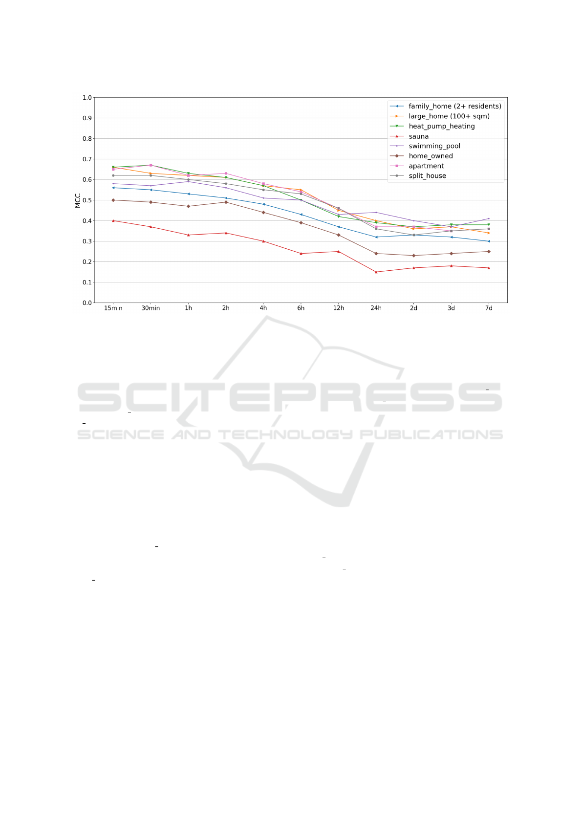
Figure 2: Matthews Correlation Coefﬁcient (MCC) for the classiﬁcation result of the

XGBoost

classiﬁer for all time granularities.

The colors represent the household-speciﬁc socio-demographic characteristics listed in the legend.

characteristics has been observed. For time granular-

ities ranging from 15 minutes to one hour, the pre-

diction performance remains consistent and achieves

similar results. However, beyond one hour, a drop

in accuracy is observed for most characteristics, ex-

cept for home owned and sauna. For example, fam-

ily home starts with an MCC of 0.57 at 15 minutes

and declines to 0.54 at one hour. To put this in to per-

spective, an MCC falling within the range of +0.7 to

+0.4 is generally considered to signify moderate clas-

siﬁcation performance, while +0.2 to +0.4 indicates

moderate performance. MCC values near 0 suggest

random guessing, and those below +0.2 indicate poor

classiﬁcation (Chicco et al., 2021).

Between a time-granularity of 2-hour and 24-

hour, the prediction performance for all selected

socio-demographic characteristics drops, signiﬁcantly.

Sauna and swimming pool performs not as consistent

as the other characteristics for this time-granularity

range. For instance, the performance of the swim-

ming pool drop considerably between 6 hours and 12

hours and increases slightly between 12 and 24 hours.

Whereas, the sauna illustrates the contrary trend and

increases slightly between 6 and 12 hours, followed

by a huge drop from 12 to 24 hours. Beyond 24 hours,

the trends remain relatively stable, with no signiﬁcant

changes for most characteristics.

A similar decline in performance over time is ob-

served for the

MLP

and

SVM

classiﬁers, although their

overall prediction performance is lower compared to

XGBoost

. The trend across time granularities remains

consistent with what is shown in Figure 2. Due to

space limitations, detailed plots for the

MLP

and

SVM

classiﬁers are provided separately in the Git repository.

Figure 3 shows a precision-over-recall analysis

for the socio-demographic characteristics large home

(left) and swimming pool (right) using the

XGBoost

classiﬁer. These characteristics have been chosen due

to their prominence in the literature (see Section 6).

The x-axis represents recall, indicating the proportion

of actual positives correctly identiﬁed, while the y-

axis represents precision, reﬂecting the proportion of

correct positive predictions.

The symbols illustrate the variation in prediction

performance with different time granularities. The

cross symbol (X) indicates the level of biased random

guessing, whose performance increases with higher

imbalance ratio of the class labels. For both charac-

teristics an increase of the time granularity reduces

both precision and recall. The impact is less severe for

large home, a more stable characteristic, compared to

swimming pool which is more variable. Despite the

decline, the classiﬁer’s performance performance re-

mains above random guessing for both characteristics.

6 DISCUSSION & COMPARISON

TO RELATED WORK

In this section, we ﬁrst summarize the results, followed

by a discussion of the limitations and a comparison

of our methodology with the most similar existing ap-

proaches. If a decision has to be made concerning the

SMARTGREENS 2025 - 14th International Conference on Smart Cities and Green ICT Systems

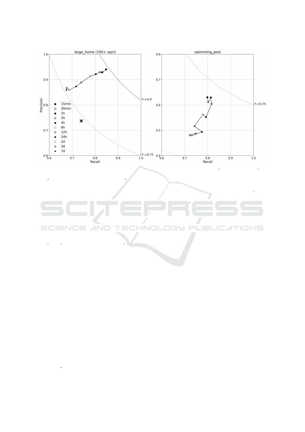
Figure 3: Prediction performance of the

XGBoost

classiﬁer as a precision-over-recall plot for large home and swimming pool.

Legend symbols represent different time granularities, with the cross symbolizing biased random guessing, visible for

large home but outside the range for swimming pool, where Recall and Precision are around 0.3.

granularity of collected load data, our ﬁndings suggest

that use cases which require data minimization or max-

imum privacy may use one-hour data without loss of

classiﬁcation performance. Conversely, for use cases

which require maximum granularity (15 minutes), e.g.,

for legal or regulatory reasons, no better prediction

performance is achieved by using higher granularity.

Best results regarding prediction performance

are exhibited for the household characteristics

heat pump heating, apartment and large home with

values between

0.6

and

0.65

, when relying on weekly

snippets with 15-minute time granularity. While vary-

ing MCC values are reported for the eight examined

household characteristics, the consistent decline in the

prediction performance across all characteristics indi-

cates that the type of characteristic being predicted is

not the most signiﬁcant factor in the trade-off between

data utility and privacy preservation. Instead, it sug-

gests that the increase in time granularity may play a

more signiﬁcant role in the change of the performance.

The approach here is limited by possible inaccu-

racy of the ground truth as the answers provided by

the participants in the questionnaire may be incorrect,

unclear, or based on estimation. Furthermore, utiliza-

tion information about household characteristics for

all single weeks is missing: the data does not specify

in which week each socio-demographic characteristic

is utilized. While some characteristics to predict are

constant for each week in the year, such as the ﬂoor

space of a house or the type of the household (apart-

ment, split house), others may ﬂuctuate such as the

number of residents present in a week (family home)

or the types of appliances in use in a given weekly snip-

pet (swimming pool or sauna). However, the dataset

is not labeled week-by-week, which prompted us to

construct labels for each week from the information

given for a household’s yearly load proﬁle. It is to be

noted that this results in some weeks possibly being

mislabeled or not containing the necessary information

for the classiﬁer to perform an informed decision on

whether a certain ﬂuctuating characteristic is present in

an arbitrary week or not. In spite of this, the classiﬁca-

tion results for all eight examined socio-demographic

household characteristics are above what is expected

from random guessing.

The approach here is also limited as it considers

features taken from (Beckel et al., 2014) which were

constructed with a time-resolution of 30 minutes as

underlying resolution in mind. Most of the computed

features are designed to capture special daily periods

i.e., the total consumption in the evening or the ratio

between the total consumption of the morning and the

total consumption of the noon. Here, these features

are used even with coarser granularities than 24 hours,

e.g., 2 days, 3 days, and 7 days. The deﬁnition of

features that are able to capture similar information

over coarser time granularities then 24 hours is future

work and need to be investigated.

As already stated in Section 2, it was not clear,

whether our methodology that uses training data of one

year and predicts a single, arbitrary week of the year

is better than the one from (Beckel et al., 2014) where

Predicting Socio-Demographic Characteristics from Load Proﬁles with Varying Time Granularities

training and testing data are from the same, single

week of the year. It turns out that our approach leads

to better performance values: the ﬁgures in (Beckel

et al., 2014) show MCC values

0.4 for the labels

familyhome (0.34), largehome (0.18), and housetype

(0.2), classiﬁed with the SVM. Our approach leads

to values up to 0.65 at the same time granularity of

30 min which are consistently higher for those labels.

While the deﬁnition of the labels are not exactly the

same it should be noted that (i) we tried to mimic the

labels from (Beckel et al., 2014) as good as possible to

enable a fair comparison (for example we did not have

information about children in our dataset) and (ii) the

choice of the thresholds did not include any kind of op-

timization with respect to classiﬁcation performance.

The inﬂuence of time granularity on socio-

demographic features differs signiﬁcantly from that

on appliance detection, as shown in the comparison

with (Eibl and Engel, 2015). In their study, time gran-

ularity starts at 3 seconds, and except for light usage,

privacy is largely preserved at our coarsest granularity

of 15 minutes. Additionally, privacy is achieved differ-

ently: while their privacy gains stem from a decrease

in recall with stable precision, in our case, both recall

and precision decline with coarser time granularities

(Figure 3).

Our prediction performance compares well

with (Ferner et al., 2019) and (Burkhart et al., 2018),

where swimming pool existence have been predicted

using load proﬁles from a whole year. Despite our

use of only a single week’s data and standard features

from (Beckel et al., 2013), our approach remains com-

petitive. For instance, while Ferner et al. achieved

0.93 accuracy and 0.67 precision using SVM with

Gaussian and handcrafted features, we obtained an

overall precision of 0.63 and accuracy of 0.81 at the

same 15-minute granularity (Ferner et al., 2019). With

XGBoost

, however, we achieve nearly the same accu-

racy of 0.92.

7 CONCLUSION & OUTLOOK

We introduce a novel evaluation methodology tai-

lored for the prediction of household-speciﬁc socio-

demographic characteristics, utilizing load proﬁles

with varying time granularities, all obtained from a

single, randomly chosen week within one year. This

sets our methodology apart from existing methods,

which either choose a speciﬁc week of the year for

both training and evaluation or employ an entire year’s

worth of data for prediction. Despite the increased

complexity of randomly selecting a week within a

year for prediction, our classiﬁcation algorithm demon-

strates improved performance for a selected subset of

household-speciﬁc socio-demographic characteristics

in comparison to the utilization of a single known week

and the application of an entire year’s data.

Our ﬁndings also indicate that, as time granu-

larity becomes coarser, progressing from 15 min-

utes to 7 days, the prediction performance for socio-

demographic characteristics generally declines notice-

ably, as expected. However, we observe two plateaus:

First, surprisingly, one-hour granularity exhibits pre-

diction performance comparable to that of 15-minute

granularity. Second, the prediction performance be-

tween 24 hours and 7 days of time granularity remains

nearly constant, possibly due to the customized design

of the numerical characteristics extracted from load

proﬁles during feature extraction. Both plateaus mean

that there are multiple intervals of granularities within

which detection performance varies only to an insignif-

icant extent. Consequently, depending on the use case,

the coarsest, the ﬁnest or any granularity within such

an interval can be chosen to achieve desired classiﬁca-

tion performance.

One limitation of our work is the custom design,

which restricts the information captured by numerical

characteristics for granularities over 24 hours. Future

research should address this and explore novel numeri-

cal representations for weekly load proﬁles to improve

the balance between data utility and privacy. Addition-

ally, incorporating advanced techniques like recurrent

autoencoders and deep neural networks could further

enhance feature extraction. One further approach for

investigation pertains to whether the observed trends

remain consistent when handling monthly, quarterly,

or yearly data snippets. Finally, there is signiﬁcant

room for improvement concerning the correct match-

ing of weekly load proﬁles to their associated socio-

demographic characteristics. We assume the charac-

teristics to be constant for the whole year, even if the

presence of some characteristics (e.g. the use of appli-

ances such as sauna or swimming pool, or the number

of residents present in a given week) may ﬂuctuate

over the course of a year, leading to incorrect training

results for the classiﬁer employed. This would require

new datasets with weekly logging of appliance uses.

ACKNOWLEDGMENTS

The ﬁnancial support by the Federal State of Salzburg

PRISMATICS research project is gratefully acknowl-

edged.

SMARTGREENS 2025 - 14th International Conference on Smart Cities and Green ICT Systems

REFERENCES

Abreu, J. M., Pereira, F. C., and Ferr

ao, P. (2012). Using

pattern recognition to identify habitual behavior in resi-

dential electricity consumption. Energy and Buildings,

49:479–487.

Alahakoon, D. and Yu, X. (2016). Smart electricity meter

data intelligence for future energy systems: A survey.

IEEE Transactions on Industrial Informatics, 12:425–

436.

Armel, K. C., Gupta, A., Shrimali, G., and Albert, A. (2013).

Is disaggregation the holy grail of energy efﬁciency?

the case of electricity. Energy Policy, 52:213–234.

Asghar, M. R., D

an, G., Miorandi, D., and Chlamtac, I.

(2017). Smart meter data privacy: A survey. IEEE

Communications Surveys Tutorials, 19:2820–2835.

Beckel, C., Kleiminger, W., Cicchetti, R., Staake, T., and

Santini, S. (2014). The eco data set and the perfor-

mance of non-intrusive load monitoring algorithms. In

Proceedings of the 1st ACM International Conference

on Embedded Systems for Energy-Efﬁcient Buildings,

BuildSys ’14, page 80–89, New York, NY, USA. Asso-

ciation for Computing Machinery.

Beckel, C., Sadamori, L., and Santini, S. (2012). Towards

automatic classiﬁcation of private households using

electricity consumption data. In Proceedings of the

Fourth ACM Workshop on Embedded Sensing Systems

for Energy-Efﬁciency in Buildings, BuildSys ’12, page

169–176, New York, NY, USA. Association for Com-

puting Machinery.

Beckel, C., Sadamori, L., and Santini, S. (2013). Automatic

socio-economic classiﬁcation of households using elec-

tricity consumption data. In Proceedings of the 4th

ACM International Conference on Future Energy Sys-

tems (e-Energy 2013), pages 75–86, New York, NY,

USA. ACM.

Birt, B. J., Newsham, G. R., Beausoleil-Morrison, I., Arm-

strong, M. M., Saldanha, N., and Rowlands, I. H.

(2012). Disaggregating categories of electrical energy

end-use from whole-house hourly data. Energy and

Buildings, 50:93–102.

Bishop, C. M. (2006). Pattern Recognition and Ma-

chine Learning (Information Science and Statistics).

Springer-Verlag, Berlin, Heidelberg.

Burkhart, S., Unterweger, A., Eibl, G., and Engel, D. (2018).

Detecting swimming pools in 15-minute load data. In

17th IEEE International Conference On Trust, Secu-

rity And Privacy In Computing And Communications

(TrustCom 2018), pages 1651–1655, New York, NY,

USA. IEEE.

Chen, D., Barker, S., Subbaswamy, A., Irwin, D., and

Shenoy, P. (2013). Non-intrusive occupancy monitor-

ing using smart meters. In Proceedings of the 5th ACM

Workshop on Embedded Systems For Energy-Efﬁcient

Buildings - BuildSys’13, pages 1–8, New York, NY,

USA. Association for Computing Machinery.

Chen, T. and Guestrin, C. (2016). Xgboost: A scalable tree

boosting system. In Proceedings of the 22nd ACM

SIGKDD International Conference on Knowledge Dis-

covery and Data Mining, KDD ’16, page 785–794,

New York, NY, USA. Association for Computing Ma-

chinery.

Chicco, D. and Jurman, G. (2020). The advantages of the

matthews correlation coefﬁcient (mcc) over f1 score

and accuracy in binary classiﬁcation evaluation. BMC

genomics, 21:1–13.

Chicco, D., Starovoitov, V. V., and Jurman, G. (2021). The

beneﬁts of the matthews correlation coefﬁcient (mcc)

over the diagnostic odds ratio (dor) in binary classiﬁca-

tion assessment. IEEE Access, 9:47112–47124.

Chicco, G. (2016). Customer behaviour and data analytics.

In 2016 International Conference and Exposition on

Electrical and Power Engineering (EPE), pages 771–

779, Iasi, Romania. IEEE.

Commission, E. (2012). 2012/148/eu: Commission recom-

mendation of 9 march 2012 on preparations for the

roll-out of smart metering systems.

Darby, S. (2010). Smart metering: What potential for house-

holder engagement? Building Research and Informa-

tion, 38:442–457.

Efthymiou, C. and Kalogridis, G. (2010). Smart grid pri-

vacy via anonymization of smart metering data. In

2010 First IEEE International Conference on Smart

Grid Communications, pages 238–243, Gaithersburg,

Maryland, USA. IEEE.

Eibl, G. and Engel, D. (2015). Inﬂuence of data granularity

on smart meter privacy. IEEE Transactions on Smart

Grid, 6:930–939.

Engel, D. and Eibl, G. (2017). Wavelet-based multiresolution

smart meter privacy. IEEE Transactions on Smart Grid,

8:1710–1721.

Erkin, Z., Troncoso-Pastoriza, J. R., Lagendijk, R. L., and

Perez-Gonzalez, F. (2013). Privacy-preserving data

aggregation in smart metering systems: An overview.

IEEE Signal Processing Magazine, 30:75–86.

Fan, Z., Kulkarni, P., Gormus, S., Efthymiou, C., Kalogridis,

G., Sooriyabandara, M., Zhu, Z., Lambotharan, S.,

and Chin, W. H. (2013). Smart grid communications:

Overview of research challenges, solutions, and stan-

dardization activities. IEEE Communications Surveys

and Tutorials, 15:21–38.

Ferner, C., Eibl, G., Unterweger, A., Burkhart, S., and We-

genkittl, S. (2019). Pool detection from smart metering

data with convolutional neural networks. Energy Infor-

matics, 2:1–9.

Finster, S. and Baumgart, I. (2014). Privacy-aware smart

metering: A survey. IEEE Communications Surveys &

Tutorials, 16:1732–1745.

Granell, R., Axon, C. J., and Wallom, D. C. (2015). Impacts

of raw data temporal resolution using selected clus-

tering methods on residential electricity load proﬁles.

IEEE Transactions on Power Systems, 30(6):3217–

3224.

Greveler, U., Justus, B., and L

ohr, D. (2012). Multime-

dia content identiﬁcation through smart meter power

usage proﬁles. In Proceedings of the International Con-

ference on Information and Knowledge Engineering

(IKE), pages 1–8, Athens, GA, USA. CSREA Press.

Hart, G. (1992). Nonintrusive appliance load monitoring.

Proceedings of the IEEE, 80(12):1870–1891.

Predicting Socio-Demographic Characteristics from Load Proﬁles with Varying Time Granularities

Haykin, S. (1998). Neural Networks: A Comprehensive

Foundation. Prentice Hall PTR, USA, 2nd edition.

He, H. and Garcia, E. (2009). Learning from imbalanced

data. Knowledge and Data Engineering, IEEE Trans-

actions on, 21:1263–1284.

Hearst, M., Dumais, S., Osuna, E., Platt, J., and Scholkopf,

B. (1998). Support vector machines. IEEE Intelligent

Systems and their Applications, 13(4):18–28.

Hernandez, J. C., Sanchez-Sutil, F., Cano-Ortega, A., and

Baier, C. R. (2020). Inﬂuence of data sampling fre-

quency on household consumption load proﬁle fea-

tures: A case study in spain. Sensors, 20:6034.

Hopf, K., Sodenkamp, M., Kozlovkiy, I., and Staake, T.

(2016). Feature extraction and ﬁltering for house-

hold classiﬁcation based on smart electricity meter

data. Computer Science - Research and Development,

31:141–148.

Huchtkoetter, J. and Reinhardt, A. (2020). On the impact

of temporal data resolution on the accuracy of non-

intrusive load monitoring. In Proceedings of the 7th

ACM International Conference on Systems for Energy-

Efﬁcient Buildings, Cities, and Transportation, pages

270–273, New York, NY, USA. Association for Com-

puting Machinery.

Japkowicz, N. (2000). The class imbalance problem: Sig-

niﬁcance and strategies. In Proc. of the Int’l Conf. on

artiﬁcial intelligence, volume 56, pages 111–117.

Kim, H., Marwah, M., Arlitt, M. F., Lyon, G., and Han,

J. (2011). Unsupervised disaggregation of low fre-

quency power measurements. In Proceedings of the

2011 SIAM International Conference on Data Mining

(SDM), pages 747–758, Mesa, Arizona, USA. SIAM /

Omnipress.

Kleiminger, W., Beckel, C., and Santini, S. (2015). House-

hold occupancy monitoring using electricity meters.

In Proceedings of the 2015 ACM International Joint

Conference on Pervasive and Ubiquitous Computing,

pages 975–986, New York, NY, USA. Association for

Computing Machinery.

Kleiminger, W., Beckel, C., Staake, T., and Santini, S.

(2013). Occupancy detection from electricity consump-

tion data. In Proceedings of the 5th ACM Workshop

on Embedded Systems For Energy-Efﬁcient Buildings,

pages 1–8, New York, NY, USA. Association for Com-

puting Machinery.

Kolter, J. Z. and Jaakkola, T. (2012). Approximate inference

in additive factorial hmms with application to energy

disaggregation. Journal of Machine Learning Research

- Proceedings Track, 22:1472–1482.

Lisovich, M., Mulligan, D., and Wicker, S. (2010). Inferring

personal information from demand-response systems.

IEEE Security & Privacy, 8:11–20.

Matthews, B. (1975). Comparison of the predicted and

observed secondary structure of t4 phage lysozyme.

Biochimica et Biophysica Acta (BBA) - Protein Struc-

ture, 405(2):442–451.

Molina-Markham, A., Shenoy, P., Fu, K., Cecchet, E., and

Irwin, D. (2010). Private memoirs of a smart meter.

In Proceedings of the 2nd ACM Workshop on Embed-

ded Sensing Systems for Energy-Efﬁciency in Building,

pages 61–66, New York, NY, USA. ACM.

Osborne, J. (2002). Notes on the use of data transformations.

Practical assessment, research, and evaluation, 8:6.

Pathak, N., Lachut, D., Roy, N., Banerjee, N., and Robucci,

R. (2018). Non-intrusive air leakage detection in resi-

dential homes. In Proceedings of the 19th International

Conference on Distributed Computing and Networking,

page 10, Varanasi, India. ACM.

Radovanovic, D., Unterweger, A., Eibl, G., Engel, D., and

Reichl, J. (2022). How unique is weekly smart meter

data? Energy Informatics, 5:1–13.

Silva, D. D., Yu, X., Alahakoon, D., and Holmes, G. (2011).

A data mining framework for electricity consumption

analysis from meter data. IEEE Transactions on Indus-

trial Informatics, 7:399–407.

Sokolova, M. and Lapalme, G. (2009). A systematic analysis

of performance measures for classiﬁcation tasks. Infor-

mation Processing and Management, 45(4):427–437.

Verdu, S. V., Garcia, M. O., Senabre, C., Marin, A. G.,

and Franco, F. J. G. (2006). Classiﬁcation, ﬁltering,

and identiﬁcation of electrical customer load patterns

through the use of self-organizing maps. IEEE Trans-

actions on Power Systems, 21:1672–1682.

Viegas, J. L., Vieira, S. M., and Sousa, J. M. (2016). Min-

ing consumer characteristics from smart metering data

through fuzzy modelling. Communications in Com-

puter and Information Science, 610:562–573.

Wang, Y., Chen, Q., Gan, D., Yang, J., Kirschen, D. S.,

and Kang, C. (2019a). Deep learning-based socio-

demographic information identiﬁcation from smart me-

ter data. IEEE Transactions on Smart Grid, 10:2593–

2602.

Wang, Y., Chen, Q., Hong, T., and Kang, C. (2019b). Review

of smart meter data analytics: Applications, method-

ologies, and challenges. IEEE Transactions on Smart

Grid, 10:3125–3148.

Weranga, K. S. K., Kumarawadu, S., and Chandima, D. P.

(2014). Smart Metering Applications. Springer Singa-

pore, Singapore.

Zeifman, M. and Roth, K. (2011). Nonintrusive appliance

load monitoring: Review and outlook. IEEE Transac-

tions on Consumer Electronics, 57:76–84.

Zoha, A., Gluhak, A., Imran, M. A., and Rajasegarar, S.

(2012). Non-intrusive load monitoring approaches for

disaggregated energy sensing: A survey. Sensors 2012,

12:16838–16866.

SMARTGREENS 2025 - 14th International Conference on Smart Cities and Green ICT Systems