Spatio-Temporal Trafﬁc Prediction for Efﬁcient ITS Management

Aram Nasser

and Vilmos Simon

Department of Networked Systems and Services, Faculty of Electrical Engineering and Informatics,

Budapest University of Technology and Economics, Budapest, H-1111, Hungary

Keywords:

Intelligent Transportation Systems, Trafﬁc Prediction, Attention, Encoder-Decoder, Spatio-Temporal Data

Presentation.

Abstract:

Trafﬁc forecasting is a crucial element of Intelligent Transportation Systems (ITSs), exerting signiﬁcant in-

ﬂuence on the optimization of urban mobility. Through precise anticipation of trafﬁc patterns, ITS facilitates

proactive trafﬁc ﬂow management, leading to a multitude of beneﬁts for both the city and its inhabitants.

However, the intricate topological structure of road networks and the changing temporal patterns in trafﬁc

create challenging problems that demand solutions considering both the spatial and temporal aspects of trafﬁc

characteristics. Most existing trafﬁc prediction models are inﬂuenced by Graph Neural Networks (GNNs) to

capture the spatial structure of road networks. However, this approach typically relies on the adjacency matrix,

which might not always reﬂect the dynamic state of trafﬁc conditions. In addition, GNNs are not universally

applicable across different trafﬁc topologies. What works for one road network may not yield the same results

for another, owing to disparities in the number of roads, thus graph nodes, and the unique characteristics of

each location. Therefore, in this paper, the Spatio-Temporal Multi-Head Attention (ST-MHA) model is in-

troduced to solve this issue. ST-MHA depends on a modiﬁed version of the Multi-Head Attention (MHA)

mechanism to capture the spatial structure of the road network implicitly, as well as a GRU-based encoder-

decoder structure for integrating the temporal characteristics. Our model outperforms three state-of-the-art

baseline models, which include temporal, spatial, and spatio-temporal models. This enhanced performance is

evident across three different prediction horizons when evaluated on a real-world trafﬁc dataset.

1 INTRODUCTION

The unprecedented expansion of cities has imposed

increased pressure on transportation networks, result-

ing in a negative inﬂuence on human health, the econ-

omy, and the environment (Levy et al., 2010), (Zhang

and Batterman, 2013). This pressure has prompted

concerned people and organizations in smart cities

to contribute to the creation of systems for utilizing

information, communication, and sensing technolo-

gies in transportation and transit systems, referred to

as Intelligent Transportation Systems (ITSs) (Wang,

2010). One of the key elements of ITSs is predict-

ing trafﬁc characteristics, such as speed, as it provides

a futuristic view of the trafﬁc situation. This insight

gives the authorities the time needed to take action be-

fore congestion arises, ultimately leading to a reduc-

tion in pollution and commute time for individuals.

The integration of innovative technologies, as well as

https://orcid.org/0000-0001-9696-7387

https://orcid.org/0000-0002-7627-3676

novel data collection techniques, like sensors (includ-

ing ﬂoating car and wide-area sensors) and connected

vehicles, have increased the complexity of analyz-

ing and managing trafﬁc data (Rahmani et al., 2023),

(Kaffash et al., 2021).

The problem of trafﬁc prediction has evolved from

a statistical challenge into a problem tackled by Ma-

chine Learning and, most recently, Deep Learning. It

can be analyzed as time series data, allowing for fu-

ture predictions based on past observations and par-

ticularly considering the evolving trafﬁc values over

time (Yuan et al., 2022). Nevertheless, in some cases,

because trafﬁc data are gathered from real spatially-

located sensors, spatial information is integrated as

an external factor to improve trafﬁc prediction. The

spatial topology of the road network can be mapped

as graphs with vertices and edges, describing the sen-

sors as well as the connections among them, respec-

tively. The initial graphs are usually built based on

adjacency matrices, which can be constructed on four

distinct bases: road-based, distance-based, similarity-

based, and dynamic matrices, according to (Jiang and

Nasser, A. and Simon, V.

Spatio-Temporal Trafﬁc Prediction for Efﬁcient ITS Management.

DOI: 10.5220/0013229700003941

Paper published under CC license (CC BY-NC-ND 4.0)

In Proceedings of the 11th International Conference on Vehicle Technology and Intelligent Transport Systems (VEHITS 2025), pages 45-53

ISBN: 978-989-758-745-0; ISSN: 2184-495X

Luo, 2022). However, although the spatial topology

of the roads is static, the connections, in reality, are

not and might be strong at some periods while weak

or negligible at others. As a result, GNNs can be per-

fect for time-static data, which is not the case in trafﬁc

prediction.

To address this concern, researchers are endeavor-

ing to integrate the temporal dimension with GNNs,

enabling dynamic adjustments of connections over

time. Most available spatio-temporal models use the

GNNs to capture the spatial features of trafﬁc data,

where the adjacency matrix is usually needed to for-

mulate the initial relationship among trafﬁc detectors.

This matrix must be prepared earlier, and its dimen-

sions are ﬁxed throughout the training process, which

restricts the ability to use the same model for different

road networks interchangeably. In other words, using

the model for another road network indicates build-

ing a new adjacency matrix speciﬁcally for that new

topology. In addition, building the adjacency matrix

can be a time-consuming task, and it varies based on

the scale. For example, for the same country, the ad-

jacency matrix used for the intra-city road network

differs from the one employed for inter-city or metro

stations.

These limitations have encouraged us to introduce

our novel model, ST-MHA, where the adjacency ma-

trix is no longer needed to capture the spatial depen-

dencies. Instead, ST-MHA can implicitly infer the

spatial topology from the data. In this manuscript,

we provide a spatio-temporal model that adjusts the

MHA mechanism to capture the spatial interactions

of data while a GRU-based encoder-decoder for the

integration of temporal information. The rest of this

article is organized as follows: the next section is ded-

icated to introducing state-of-the-art literature on traf-

ﬁc prediction models, encompassing spatial, tempo-

ral, and spatio-temporal aspects. The detailed struc-

ture of ST-MHA, along with the elucidation of the

problem addressed by our model, is outlined in sec-

tion 3. In the following chapter, the experimental

setup, including the utilized dataset, evaluation met-

rics, and parameter designing, as well as the ﬁnal re-

sults and discussions, are examined in 4. Finally, the

conclusion of our research is presented in the last sec-

tion.

2 RELATED WORK

Classic statistical models, like the ARIMA model and

its variants, have been widely used in the past to an-

alyze and predict future trafﬁc status (Ahmed and

Cook, 1979), (Levin and Tsao, 1980), (Lee and Fam-

bro, 1999), (Williams, 2001), (Williams and Hoel,

2003), (Kamarianakis and Prastacos, 2003). How-

ever, these models assume the time series to be sta-

tionary (Karlaftis and Vlahogianni, 2011), (Li and

Shahabi, 2018), which hinders the trafﬁc prediction

process. Thus, the advancement of non-parametric

models, such as Support Vector Regression (SVR)

(Castro-Neto et al., 2009), (Su et al., 2007), (Jin

et al., 2007), and Neural Networks (NNs) (Hua

and Faghri, 1994), (Dougherty and Cobbett, 1997),

(Ledoux, 1997), with improved efﬁciency and height-

ened predictive precision, has made statistical mod-

els less common, especially for complex data model-

ing. Initial non-parametric models have vigorously

challenged the classical parametric models. How-

ever, when it comes to handling temporal data, even

these models have their limitations due to the time-

based associations among time steps. This issue

prompted the introduction of Recurrent Neural Net-

work (RNN) (Rumelhart et al., 1986), a special type

of NNs equipped with memory cells to help cap-

ture the temporal features of the time series. Nev-

ertheless, the vanilla RNN suffers from the vanish-

ing gradient problem (Hochreiter, 1998) that is miti-

gated by its variants like the Long-Short Term Mem-

ory (LSTM) (Hochreiter and Schmidhuber, 1997) and

Gated Recurrent Unit (GRU) (Cho et al., 2014a).

These RNNs can also be structured as models like

the RNN Encoder-Decoder architecture (Cho et al.,

2014b) to allow for a deeper structure and additional

improvement of trafﬁc prediction. While these mod-

els successfully address the trafﬁc prediction issue as

a temporal problem, some models integrated the spa-

tial features as exogenous inputs to capitalize on the

spatial interactions among roads in the road network.

To fully leverage spatial features of the road net-

work, some researchers use modiﬁed versions of the

GNNs (Gori et al., 2005) to capture adjacent inter-

actions among distinct roads in the road network.

These models are extended by integrating Convolu-

tional Neural Networks(CNNs) (Lecun et al., 1998),

in both the spectral and time domains, with GNNs to

allow the extraction of multi-scale localized spatial

features and form GCNs (Kipf and Welling, 2017),

(Zhou et al., 2020). Other GNNs can also be ex-

tended by using the attention mechanism to over-

come the shortcomings of convolution-based GNNs

(Veli

ckovi

c et al., 2017). According to (Veli

ckovi

et al., 2017), these drawbacks are solved by calcu-

lating different weights to various nodes in a neigh-

borhood implicitly and avoiding the dependence on

knowing the graph structure upfront. Nonetheless,

these models lack the ability to capture the tempo-

ral features of trafﬁc. Thus, incorporating models that

VEHITS 2025 - 11th International Conference on Vehicle Technology and Intelligent Transport Systems

consider both time and space is essential to tackle the

spatio-temporal problem.

Harnessing the advantages of both temporal and

spatial characteristics of trafﬁc data through the inte-

gration of these features into spatio-temporal models

has gained signiﬁcant attention among researchers. In

(Zhao et al., 2020), GCNs are combined with GRU

units to simultaneously capture the spatial and tem-

poral dependencies within trafﬁc data, respectively.

The authors then extended the model by incorporating

the attention mechanism into the existing framework

to improve prediction accuracy (Bai et al., 2021).

Trafﬁc ﬂow spatio-temporal dynamics are modeled as

a diffusion process in (Li et al., 2018), where spa-

tial interdependence is grasped through bidirectional

random walks on graphs and temporal interdepen-

dence is handled by employing the encoder-decoder

architecture with scheduled sampling. Dynamic Time

Warping (DTW), a technique used for matching and

alignment, is utilized and improved to what is called

“fast-DTW” to generate temporal graphs (Li and Zhu,

2021). These temporal graphs are then incorporated

into a novel Spatio-Temporal Fusion Graph Neural

(STFGN) model. Several STFGN are treated in par-

allel and their outputs are concatenated and added

with Gated CNN output to act as the input of the

next STFGN layer. Authors of SST-GNN (Roy et al.,

2021) introduce a streamlined framework that encap-

sulates two different models, current-day and histor-

ical, to capture daily and weekly patterns of traf-

ﬁc data via a weighted spatio-temporal aggregation

scheme. In (Chen et al., 2019), the authors intro-

duced the MRA-BGCN model, which is comprised

of two parts. The ﬁrst incorporates two graphs, node

and edge-wise graphs, and provides explicit model-

ing of interactions among nodes and edges. The sec-

ond is to autonomously learn the signiﬁcance of dis-

tinct neighborhood ranges. In LSGCN (Huang et al.,

2020), a new graph attention network, called cosAtt,

is combined with GCN to grasp the spatial features

of trafﬁc. In addition, a Gated Linear Unit (GLU)

is adopted for the temporal characteristics simulta-

neously. Zheng et. al. introduced GMAN (Zheng

et al., 2020), where spatio-temporal correlations are

modeled by employing an encoder-decoder architec-

ture that combines several spatio-temporal attention

mechanism blocks. Furthermore, a transform atten-

tion layer is devised between the encoder and the de-

coder to mitigate the impact of error propagation to

enhance long-term prediction performance. A variant

of the GCN, called LPGCN, is introduced in (Qi et al.,

2022) to model the spatial characteristics of trafﬁc.

On the other hand, a multi-path CNN is utilized to

learn the collective inﬂuence of past trafﬁc conditions

on future ones, which is further modiﬁed by an at-

tention mechanism. All the aforementioned spatio-

temporal models use adjacency matrices to construct

the GNNs and GCNs used in their models. These ad-

jacency matrices have their limitations, as mentioned

earlier, in addition to their impracticality while deal-

ing with large and sparse graphs -due to the large

number of zeros they might have in this case. In this

paper, the ST-MHA model is introduced to capture

both spatial and temporal features of trafﬁc data by

utilizing a modiﬁed version of the MHA mechanism

and GRU-based encoder-decoder, respectively.

3 METHODOLOGY

The full architecture of the Spatio-Temporal Multi-

Head Attention Based Trafﬁc prediction model is out-

lined in Fig. 1, where each block represents a speciﬁc

stage of the model. The lower part of each stage delin-

eates its inputs for each time step, the middle segment

displays its outputs, and the upper section indicates its

name. These stages are grouped into two components:

Spatial and Temporal. Further elaboration on these

components and their sections is provided in subse-

quent sub-sections 3.2 and 3.3, respectively. Never-

theless, before diving into the details of ST-MHA, the

problem this paper addresses is deﬁned in the next

subsection 3.1.

3.1 Problem Deﬁnition and Statement

This paper addresses the problem of estimating fu-

ture trafﬁc speeds over a given time horizon based on

present and past data. The data are collected from

multiple speed loop detectors positioned in various lo-

cations, and the objective is to capture this spatial dis-

tribution without relying on predeﬁned graph struc-

tures. This spatial modeling is then integrated with a

temporal representation of data to achieve a compre-

hensive spatio-temporal framework for representation

and prediction.

Given T current and historical time steps

(t−T −1)

, ...., X

(t−1)

, X

}, where X is the trafﬁc data

of N roads, the aim is to predict future trafﬁc data

(t+1)

, ..., X

(t+τ)

}, where τ is the prediction horizon.

While this issue can be approached as a time series

problem, the integration of the spatial features could

improve trafﬁc forecasting accuracy. The objective

of our proposed model, ST-MHA, is to utilize im-

plicit spatial and temporal patterns without the need

for creating graph structures that are restricted by the

number of nodes. To achieve that, our approach in-

volves employing a modiﬁed MHA model to capture

Spatio-Temporal Trafﬁc Prediction for Efﬁcient ITS Management

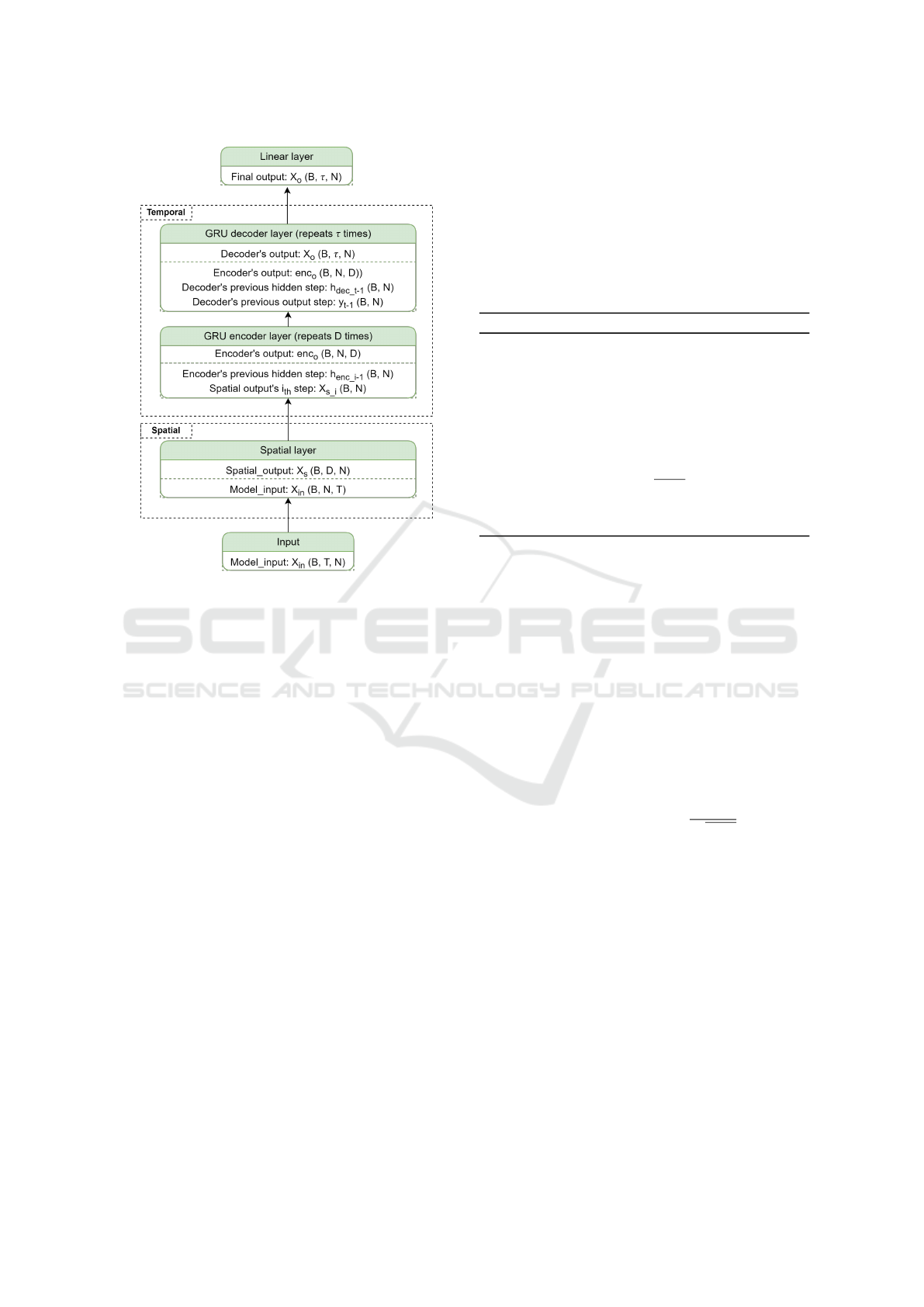
Figure 1: ST-MHA model.

the spatial properties, as well as integrating a GRU-

based encoder-decoder model to handle the temporal

characteristics.

Our model can improve trafﬁc management by

helping authorities make informed decisions to re-

duce congestion, optimize trafﬁc ﬂow, and support

route planning for mapping applications. By predict-

ing trafﬁc speeds, it provides real-time insights, al-

lowing authorities to adjust signal timings, optimize

light cycles, and implement diversions to minimize

delays. This leads to smoother trafﬁc movement,

fewer bottlenecks, and more efﬁcient travel for all

road users.

3.2 The Spatial Component

To obtain the spatial properties of trafﬁc data with-

out relying on adjacency matrices or building graph

neural networks, the interactions among several road

detectors’ data are computed over the time dimension

spanning H periods, called “heads.” In other words,

the input time series is divided into several heads,

each describing distinct periods of the past data. Nev-

ertheless, this direct approach has two problems. The

ﬁrst one arises when the available historical data are

scarce, which might make it challenging to partition

the data into segments. The second involves the care-

ful consideration of the number of input time steps,

ensuring that this number is divisible by the number

of heads H. Failing to meet this condition can lead to

the failure of the whole model. To solve these issues

and minimize the dependence on a varying number of

past time steps, the time dimension is mapped onto

the size of the model’s hidden dimension. Therefore,

the interactions are rendered within a consistent di-

mension, typically larger than the initial one.

Algorithm 1: Spatial Component.

Input: Input sequence X

Data: Model’s hidden size D, Number of

heads H

Result: Output sequence X

X ← Linear(X

) // Mapped input

Q ← Linear

(X) // Queries

K ← Linear

(X) // Keys

V ← Linear

(X) // Values

scores ← (Q · K)/

D/H // Scores

att

← Softmax(scores)

← ReLU(concat[W

att

·V ])

Following the extension of the time dimension,

the scaled dot product MHA mechanism is utilized

as described in equations 1 and 2, akin to the MHA

model in (Vaswani et al., 2017). The input time se-

ries are projected on three linear layers, yielding the

Query, Key, and Value matrices, denoted as Q, K, and

V, respectively. Subsequently, each of these matrices

is further reshaped and divided into H heads depict-

ing various periods of the past time steps. Each at-

tention head, AH

hereafter, discerns speciﬁc depen-

dencies within the input time series, thus allowing the

model to learn different representations of the input

by attending to different parts of the sequence.

) = so f tmax(

D/H

) ∗V

(1)

MHA(Q,K,V ) = Relu(concat[AH

,...., AH

]) (2)

To capture the interactions among the road data,

D/H matrix multiplications are undertaken between

Q and K in parallel. After that, the Softmax func-

tion is utilized to constrain the outputs between zero

and one. This operation yields a matrix, denoted as

attn

, whose dimensions are (B, D/H, N, N), where

N is the number of trafﬁc detectors, illustrating how

trafﬁc data spatially inﬂuence each other interchange-

ably over H time periods. Subsequently, this matrix

is used to scale the V matrix by another matrix-to-

matrix multiplication. The outcome of this process

is a scaled representation of the input matrix, which

VEHITS 2025 - 11th International Conference on Vehicle Technology and Intelligent Transport Systems

varies based on the importance of each trafﬁc detec-

tor’s inﬂuence on the rest. It is noteworthy to men-

tion that the values obtained from the matrix multi-

plication of Q and K are divided by the square root

of D/H to avoid a potentially large magnitude of the

dot product, which might push the Softmax function

into regions with exceedingly low gradients. These

interactions are then concatenated and processed with

the Relu activation function (Agarap, 2018) to form

the modiﬁed MHA. For a deeper understanding, the

pseudo code that describes the spatial component of

ST-MHA is given in algorithm 1.

3.3 The Temporal Component

The temporal part is a GRU-based encoder-decoder

model. Before delving into the details of this com-

ponent, it is important to clarify that the GRU cell

incorporates multiple gates as described in equation

(3)(ArunKumar et al., 2022):

= σ (W

∗ [h

t−1

])

= σ (W

∗ [h

t−1

])

= tanh(W ∗ [r

∗ h

t−1

])

= (1 − z

) ∗ h

t−1

+ z

∗

(3)

where x

is the input at time t. z

and r

are the update

and reset gates at time t, respectively. h

is the hidden

state at time t, while

is the new candidate mem-

ory cell at time t. Symbols (σ) and (tanh) denote the

Sigmoid and hyperbolic tangent activation functions,

respectively, whereas ([;]) and (∗) represent concate-

nation and the element-wise multiplication.

The encoder is simply a GRU layer used to se-

quentially encode the outputs of the spatial compo-

nent with a zero-initiated hidden state. It iterates over

the spatial component’s output as described in equa-

tion 3. The decoder alters the concatenation-based at-

tention weights stated in (Luong et al., 2015). This

attention mechanism is chosen here to offer a straight-

forward approach for generating the temporal output,

one step at a time. The decoder’s hidden state at time

t-1, h

dec

t−1

is considered as the query q, and the en-

coder’s hidden states, enc

, as the keys K. This pro-

cess is done by concatenating the query and keys, the

parenthesis [;] in Algorithm 2, and applying a linear

layer followed by Softmax. Since there is no h

dec

t−1

the beginning of the process, it is initialized with the

last encoder’s hidden state, h

enc

D−1

. The resulting at-

tention weights are then multiplied with the previous

output of the model, y

t−1

, which is considered as the

values matrix V, unlike the traditional mechanism that

considers h

dec

t−1

to be the V. At this step, the GRU

cell is utilized as stated in equation 3, where the input

Algorithm 2: Temporal component.

Input: Input sequence X

Result: Output sequence X

Encoder:

for i = 0 to D do

enc

← GRUCell(X

enc

i−1

)

enc

i−1

← h

enc

← append(h

enc

)

end

Decoder:

for t ← 0 to τ do

scores ← Linear(concat[h

dec

t−1

,enc

])

← So f tmax(scores)

gru

← w

· y

t−1

dec

← GRUCell(y

t−1

gru

)

← Linear(h

dec

)

t−1

← X

← append(X

)

end

is the previous model’s output and the hidden state is

the result of the attention mechanism. The output of

each iteration is then concatenated to form the ﬁnal

output of the model. A comprehensive elucidation of

the temporal aspect and matrix dimensions at every

step is offered in algorithm 2.

4 PRACTICAL ANALYSIS

4.1 Dataset

ST-MHA is trained and evaluated on a real-world

dataset collected from the highways of Los Angeles

city via loop detectors. As in (Zhao et al., 2020),

speed data of N=207 detectors are chosen from the

1st of March till the 7th of March, 2012. Missing data

were amputated using linear interpolation. The result-

ing values are normalized between zero and one, then

reverted to their original scale at the end of the train-

ing for better results interpretation. Fig. 2 illustrates

the distribution of the road detectors over the city of

Los Angeles (Lu et al., 2020).

Trafﬁc speeds are aggregated every 5 minutes to

form 2016 data points for each trafﬁc speed detec-

tor, where the training is run on 80% of the data or

1612*207 points. The remaining 20%, or 404*207

points, are used to evaluate the model. Two hours of

past data are used as inputs to predict the next 15, 30,

and 45 minutes of future trafﬁc speeds.

Spatio-Temporal Trafﬁc Prediction for Efﬁcient ITS Management

Figure 2: Distribution of detectors over the highways of Los

Angeles County (METR-LA).

4.2 Evaluation Metrics

Four evaluation metrics are used to evaluate the per-

formance of the ST-MHA model based on ground

truth values Y

and predicted ones

. These met-

rics are the Mean Squared Error (MSE), Root Mean

Squared Error (RMSE), Mean Absolute Error (MAE),

and Mean Absolute Percentage Error (MAPE), which

are given as in the equations 4, 5, 6, and 7, respec-

tively. MSE is the average of the squared differences

between the actual and predicted values, offering a

measure to assess the average squared deviation be-

tween ground truth and predictions. However, its in-

terpretability is hindered by the squaring operation.

RMSE is the square root of MSE, and it shares the

same unit as the original data, making it more inter-

pretable. Both MSE and RMSE give higher weight to

large errors due to squaring, making them sensitive to

outliers. MAE, on the other hand, represents the aver-

age of the absolute differences between the actual and

estimated values. MAE is less sensitive to outliers

compared to MSE and RMSE and is often preferred

when outliers are present and a more balanced view

of the errors is needed. MAPE is a percentage that

describes the size of the errors compared to the actual

values. MAPE has a big limit when actual values are

close to zero, which can produce an overshoot MAPE

value. Therefore, zero values in Y were exempt while

calculating the MAPE.

MSE =

∑

i=1

− ˆy

)

(4)

RMSE =

∑

i=1

− ˆy

)

(5)

MAE =

∑

i=1

− ˆy

) (6)

MAPE =

100

∑

i=1

− ˆy

(7)

4.3 Model Parameters Designing

Two of the main parameters of ST-MHA are the

model’s hidden size and the number of heads H.

Each one of these parameters can signiﬁcantly affect

the prediction results of ST-MHA. After conducting

many experiments, the hidden size of D=128 units

and H=8 are chosen as they provide the best perfor-

mance results. Another less important parameter is

the learning rate, lr hereafter, which describes the step

by which the model is modiﬁed. lr is initiated to 0.01

and is decreased by 90% every 1000 iterations.

Due to the limited number of data samples in the

time domain, the batch size is chosen to be relatively

small, at eight samples per iteration, to enable a larger

number of training iterations per epoch. All experi-

ments are conducted over 200 epochs, where 24 past

values (equivalent to 2 hours) are used as inputs into

the model, while the prediction horizons utilized as

outputs are 15, 30, and 45 minutes.

4.4 Results and Discussion

Three benchmark models are employed to validate

our model, ST-MHA. These models are chosen to

cover the temporal, spatial, and spatio-temporal ap-

proaches. The ﬁrst is an RNN Encoder–Decoder

model (Cho et al., 2014b), encoder-decoder hereafter,

where vanilla RNNs are replaced with GRU units for

better prediction accuracy. Second is a GCN model

(Kipf and Welling, 2017) that uses the spatial fea-

tures to predict future trafﬁc speeds. The third is the

state-of-the-art spatio-temporal model TGCN, which

is conﬁgured with a model’s hidden size of 64, as re-

ported by the authors, to achieve the best results (Zhao

et al., 2020). As shown in Table 1, our model pro-

duced superior results in all metrics with relatively

stable outcomes as the prediction horizon increases.

The spatial model, GCN, demonstrates relatively

stable results, where the difference in training results

does not dramatically change as the prediction hori-

zon increases. Yet, it still performs poorer than the

temporal model when dealing with a short predic-

tion horizon at a 15-minute horizon. Nevertheless,

ST-MHA achieved improved prediction accuracy by

at least 26.43%, 14.23%, 21.47%, and 18.57% for

MSE, RMSE, MAE, and MAPE, respectively, across

all prediction horizons.

The encoder-decoder model showed relatively

good results for a short prediction period, while it

struggles to forecast longer horizons. ST-MHA per-

formed better than the encoder-decoder model in all

horizons and metrics. With ST-MHA, MSE, RMSE,

MAE, and MAPE are decreased by 12.65%, 6.55%,

VEHITS 2025 - 11th International Conference on Vehicle Technology and Intelligent Transport Systems

Table 1: Prediction results for 15, 30, and 45 minutes.

15 min encoder-decoder GCN TGCN ST-MHA

MSE 53.59 67.92 54.76 46.81

RMSE 7.32 8.24 7.4 6.84

MAE 4.56 5.63 5.085 4.38

MAPE 13.52% 15.6% 14.086% 12.003%

30 min encoder-decoder GCN TGCN ST-MHA

MSE 102.07 78.5 77.93 55.88

RMSE 10.1 8.86 8.83 7.47

MAE 6.38 5.94 6.07 4.55

MAPE 20.22% 17.17% 17.83% 13.98%

45 min encoder-decoder GCN TGCN ST-MHA

MSE 113.72 87.41 88.79 64.3

RMSE 10.66 9.34 9.42 8.01

MAE 7.1 6.24 6.39 4.9

MAPE 20.8% 18.35% 19.3 % 14.44%

3.94%, and 11.22%, respectively, for the 15-minute

prediction horizon, while attaining a reduction of

45.25%, 26.03%, 28.68%, 30.86%, respectively, for

the 30-minute, and 43.45%, 24.85%, 30.98%, and

30.57%, for the 45-minute forecasting horizon.

Compared to the TGCN model, ST-MHA scored

a drop of 14.51%, 7.56%, 13.86%, and 14.78% on

MSE, RMSE, MAE, and MAPE, respectively, for the

15-minute prediction horizon. And the enhancement

is becoming better for larger prediction horizons.

For the 30-minute prediction horizon, for example,

ST-MHA achieved a decrease of 28.29%, 15.402%,

25.04%, and 21.59% in MSE, RMSE, MAE, and

MAPE, respectively, while for the 45-minute horizon

is 27.58%, 14.96%, 23.31%, 25.18%, respectively.

Our algorithm runs fast, making it suitable for

real-time trafﬁc prediction. For example, for a 15-

minute prediction horizon, it takes 06.66 seconds to

predict future values. Given that the sample size is 5

minutes, predictions can be made while new samples

are being received, ensuring real-time functionality.

5 CONCLUSIONS

This paper presents the novel Spatio-Temporal Multi-

Head Attention model, ST-MHA, to solve the prob-

lem of jointly incorporating spatial and temporal traf-

ﬁc characteristics without relying on initial adjacency

matrices or utilizing graph structures. Instead, spa-

tial characteristics are captured internally through

the modiﬁed multi-head attention mechanism, which

considers the interactions among trafﬁc speeds over

various time segments, referred to as heads. Our

model incorporates this information with the temporal

component to accurately predict future trafﬁc speeds.

Employing ST-MHA can signiﬁcantly help to manage

and improve trafﬁc conditions, a critical aspect of In-

telligent Transportation Systems (ITS). By accurately

predicting trafﬁc patterns, authorities gain valuable

insights to make well-informed decisions aimed at al-

leviating congestion and enhancing trafﬁc ﬂow. To

ensure the efﬁciency of our model, ST-MHA is com-

pared with three baseline models: one employs tem-

poral data, another utilizes spatial data, and the third

uses spatio-temporal data. Our model demonstrates

signiﬁcant improvement over these models across

various prediction horizons in four key metrics: MSE,

RMSE, MAE, and MAPE. Although our method is

computationally efﬁcient, integrating lower-cost at-

tention techniques, such as sparse attention, could im-

prove its functionality for longer sequences and pro-

vide a promising avenue for future research.

REFERENCES

Agarap, A. F. (2018). Deep learning using rectiﬁed linear

units (relu). arXiv preprint arXiv:1803.08375.

Ahmed, M. S. and Cook, A. R. (1979). Analysis of free-

way trafﬁc time-series data by using Box-Jenkins tech-

niques. Number 722.

ArunKumar, K., Kalaga, D. V., Mohan Sai Kumar, C.,

Kawaji, M., and Brenza, T. M. (2022). Compar-

ative analysis of gated recurrent units (gru), long

short-term memory (lstm) cells, autoregressive inte-

grated moving average (arima), seasonal autoregres-

sive integrated moving average (sarima) for forecast-

ing covid-19 trends. Alexandria Engineering Journal,

61(10):7585–7603.

Bai, J., Zhu, J., Song, Y., Zhao, L., Hou, Z., Du, R., and Li,

H. (2021). A3t-gcn: Attention temporal graph convo-

lutional network for trafﬁc forecasting. ISPRS Inter-

national Journal of Geo-Information, 10(7).

Spatio-Temporal Trafﬁc Prediction for Efﬁcient ITS Management

Castro-Neto, M., Jeong, Y.-S., Jeong, M.-K., and Han, L. D.

(2009). Online-svr for short-term trafﬁc ﬂow predic-

tion under typical and atypical trafﬁc conditions. Ex-

pert systems with applications, 36(3):6164–6173.

Chen, W., Chen, L., Xie, Y., Cao, W., Gao, Y., and Feng,

X. (2019). Multi-range attentive bicomponent graph

convolutional network for trafﬁc forecasting. In AAAI

Conference on Artiﬁcial Intelligence.

Cho, K., Van Merri

enboer, B., Bahdanau, D., and Bengio,

Y. (2014a). On the properties of neural machine trans-

lation: Encoder-decoder approaches. arXiv preprint

arXiv:1409.1259.

Cho, K., Van Merri

enboer, B., Gulcehre, C., Bahdanau, D.,

Bougares, F., Schwenk, H., and Bengio, Y. (2014b).

Learning phrase representations using rnn encoder-

decoder for statistical machine translation. arXiv

preprint arXiv:1406.1078.

Dougherty, M. S. and Cobbett, M. R. (1997). Short-term

inter-urban trafﬁc forecasts using neural networks. In-

ternational journal of forecasting, 13(1):21–31.

Gori, M., Monfardini, G., and Scarselli, F. (2005). A new

model for learning in graph domains. In Proceedings.

2005 IEEE International Joint Conference on Neural

Networks, 2005., volume 2, pages 729–734 vol. 2.

Hochreiter, S. (1998). The vanishing gradient problem dur-

ing learning recurrent neural nets and problem solu-

tions. International Journal of Uncertainty, Fuzziness

and Knowledge-Based Systems, 6(02):107–116.

Hochreiter, S. and Schmidhuber, J. (1997). Long short-term

memory. Neural computation, 9(8):1735–1780.

Hua, J. and Faghri, A. (1994). Apphcations of artiﬁcial neu-

ral networks to intelligent vehicle-highway systems.

Transportation Research Record, 1453:83.

Huang, R., Huang, C., Liu, Y., Dai, G., and Kong, W.

(2020). Lsgcn: Long short-term trafﬁc prediction with

graph convolutional networks. In IJCAI, volume 7,

pages 2355–2361.

Jiang, W. and Luo, J. (2022). Graph neural network for

trafﬁc forecasting: A survey. Expert Systems with Ap-

plications, 207:117921.

Jin, X., Zhang, Y., and Yao, D. (2007). Simultaneously pre-

diction of network trafﬁc ﬂow based on pca-svr. In

Advances in Neural Networks–ISNN 2007: 4th Inter-

national Symposium on Neural Networks, ISNN 2007,

Nanjing, China, June 3-7, 2007, Proceedings, Part II

4, pages 1022–1031. Springer.

Kaffash, S., Nguyen, A. T., and Zhu, J. (2021). Big data al-

gorithms and applications in intelligent transportation

system: A review and bibliometric analysis. Interna-

tional Journal of Production Economics, 231:107868.

Kamarianakis, Y. and Prastacos, P. (2003). Forecasting traf-

ﬁc ﬂow conditions in an urban network: Compari-

son of multivariate and univariate approaches. Trans-

portation Research Record, 1857(1):74–84.

Karlaftis, M. G. and Vlahogianni, E. I. (2011). Statisti-

cal methods versus neural networks in transportation

research: Differences, similarities and some insights.

Transportation Research Part C: Emerging Technolo-

gies, 19(3):387–399.

Kipf, T. N. and Welling, M. (2017). Semi-Supervised Clas-

siﬁcation with Graph Convolutional Networks. In

Proceedings of the 5th International Conference on

Learning Representations, ICLR ’17.

Lecun, Y., Bottou, L., Bengio, Y., and Haffner, P. (1998).

Gradient-based learning applied to document recogni-

tion. Proceedings of the IEEE, 86(11):2278–2324.

Ledoux, C. (1997). An urban trafﬁc ﬂow model integrat-

ing neural networks. Transportation Research Part C:

Emerging Technologies, 5(5):287–300.

Lee, S. and Fambro, D. B. (1999). Application of subset

autoregressive integrated moving average model for

short-term freeway trafﬁc volume forecasting. Trans-

portation research record, 1678(1):179–188.

Levin, M. and Tsao, Y.-D. (1980). On forecasting freeway

occupancies and volumes (abridgment). Transporta-

tion Research Record, (773).

Levy, J. I., Buonocore, J. J., and Von Stackelberg, K. (2010).

Evaluation of the public health impacts of trafﬁc con-

gestion: a health risk assessment. Environmental

health, 9:1–12.

Li, M. and Zhu, Z. (2021). Spatial-temporal fusion graph

neural networks for trafﬁc ﬂow forecasting. Proceed-

ings of the AAAI Conference on Artiﬁcial Intelligence,

35(5):4189–4196.

Li, Y. and Shahabi, C. (2018). A brief overview of machine

learning methods for short-term trafﬁc forecasting and

future directions. Sigspatial Special, 10(1):3–9.

Li, Y., Yu, R., Shahabi, C., and Liu, Y. (2018). Diffusion

convolutional recurrent neural network: Data-driven

trafﬁc forecasting. In International Conference on

Learning Representations.

Lu, H., Huang, D., Song, Y., Jiang, D., Zhou, T., and Qin, J.

(2020). St-trafﬁcnet: A spatial-temporal deep learning

network for trafﬁc forecasting. Electronics, 9(9).

Luong, M.-T., Pham, H., and Manning, C. D. (2015). Ef-

fective approaches to attention-based neural machine

translation. arXiv preprint arXiv:1508.04025.

Qi, J., Zhao, Z., Tanin, E., Cui, T., Nassir, N., and Sarvi,

M. (2022). A graph and attentive multi-path convo-

lutional network for trafﬁc prediction. IEEE Transac-

tions on Knowledge and Data Engineering.

Rahmani, S., Baghbani, A., Bouguila, N., and Patterson, Z.

(2023). Graph neural networks for intelligent trans-

portation systems: A survey. IEEE Transactions on

Intelligent Transportation Systems, 24(8):8846–8885.

Roy, A., Roy, K. K., Ahsan Ali, A., Amin, M. A., and Rah-

man, A. K. M. M. (2021). Sst-gnn: Simpliﬁed spatio-

temporal trafﬁc forecasting model using graph neural

network. In Karlapalem, K., Cheng, H., Ramakrish-

nan, N., Agrawal, R. K., Reddy, P. K., Srivastava, J.,

and Chakraborty, T., editors, Advances in Knowledge

Discovery and Data Mining, pages 90–102, Cham.

Springer International Publishing.

Rumelhart, D. E., Hinton, G. E., and Williams, R. J. (1986).

Learning representations by back-propagating errors.

nature, 323(6088):533–536.

Su, H., Zhang, L., and Yu, S. (2007). Short-term trafﬁc

ﬂow prediction based on incremental support vector

VEHITS 2025 - 11th International Conference on Vehicle Technology and Intelligent Transport Systems

regression. In Third international conference on natu-

ral computation (ICNC 2007), volume 1, pages 640–

645. IEEE.

Vaswani, A., Shazeer, N., Parmar, N., Uszkoreit, J., Jones,

L., Gomez, A. N., Kaiser, Ł., and Polosukhin, I.

(2017). Attention is all you need. Advances in neural

information processing systems, 30.

Veli

ckovi

c, P., Cucurull, G., Casanova, A., Romero, A., Lio,

P., and Bengio, Y. (2017). Graph attention networks.

arXiv preprint arXiv:1710.10903.

Wang, F.-Y. (2010). Parallel control and management for

intelligent transportation systems: Concepts, architec-

tures, and applications. IEEE Transactions on Intelli-

gent Transportation Systems, 11(3):630–638.

Williams, B. M. (2001). Multivariate vehicular trafﬁc ﬂow

prediction: evaluation of arimax modeling. Trans-

portation Research Record, 1776(1):194–200.

Williams, B. M. and Hoel, L. A. (2003). Modeling and fore-

casting vehicular trafﬁc ﬂow as a seasonal arima pro-

cess: Theoretical basis and empirical results. Journal

of transportation engineering, 129(6):664–672.

Yuan, T., Da Rocha Neto, W., Rothenberg, C. E., Obraczka,

K., Barakat, C., and Turletti, T. (2022). Machine

learning for next-generation intelligent transporta-

tion systems: A survey. Transactions on emerging

telecommunications technologies, 33(4):e4427.

Zhang, K. and Batterman, S. (2013). Air pollution and

health risks due to vehicle trafﬁc. Science of the to-

tal Environment, 450:307–316.

Zhao, L., Song, Y., Zhang, C., Liu, Y., Wang, P., Lin,

T., Deng, M., and Li, H. (2020). T-gcn: A tempo-

ral graph convolutional network for trafﬁc prediction.

IEEE Transactions on Intelligent Transportation Sys-

tems, 21(9):3848–3858.

Zheng, C., Fan, X., Wang, C., and Qi, J. (2020). Gman:

A graph multi-attention network for trafﬁc prediction.

In Proceedings of the AAAI conference on artiﬁcial

intelligence, volume 34, pages 1234–1241.

Zhou, J., Cui, G., Hu, S., Zhang, Z., Yang, C., Liu, Z.,

Wang, L., Li, C., and Sun, M. (2020). Graph neu-

ral networks: A review of methods and applications.

AI Open, 1:57–81.

Spatio-Temporal Trafﬁc Prediction for Efﬁcient ITS Management

REFERENCES

Agarap, A. F. (2018). Deep learning using rectified linear