Agile Effort Estimation Improved by Feature Selection and Model
Explainability
V
´
ıctor P
´
erez-Piqueras
a
, Pablo Bermejo L
´
opez
b
and Jos
´
e A. G
´
amez
c
Computing Systems Department, Universidad de Castilla-La Mancha, Spain
Keywords:
Software Effort Estimation, Feature Subset Selection, Explainability.
Abstract:
Agile methodologies are widely adopted in the industry, with iterative development being a common practice.
However, this approach introduces certain risks in controlling and managing the planned scope for delivery at
the end of each iteration. Previous studies have proposed machine learning methods to predict the likelihood
of meeting this committed scope, using models trained on features extracted from prior iterations and their
associated tasks. A crucial aspect of any predictive model is user trust, which depends on the model’s explain-
ability. However, an excessive number of features can complicate interpretation. In this work, we propose
feature subset selection methods to reduce the number of features without compromising model performance.
To ensure interpretability, we leverage state-of-the-art explainability techniques to analyze the key features
driving model predictions. Our evaluation, conducted on five large open-source projects from prior studies,
demonstrates successful feature subset selection, reducing the feature set to 10% of its original size without
any loss in predictive performance. Using explainability tools, we provide a synthesis of the features with the
most significant impact on iteration performance predictions across agile projects.
1 INTRODUCTION
Software project management is a crucial and risky
process in the development of any software. Over
time, agile methodologies have been widely adopted,
as documented by the 17th State of Agile Report
(Digital.ai, 2023), which shows that 71 percent of
organizations report using agile methods. One of
the core practices in agile is iterative development,
achieved by splitting work into sprints to avoid long-
term, high-risk planning. These iterations typically
last between two and four weeks. During the planning
of an iteration, it is common to define and refine the
tasks to be completed. As part of this task refinement,
effort estimation is often performed, offering several
benefits: first, it encourages the team to discuss the
task and reach a shared understanding; second, the
estimate helps decide whether to include a particu-
lar task in the iteration, based on the team’s capacity
and the balance between the task’s expected value and
the effort required to implement it. As a result, effort
estimation is regularly carried out by teams through-
a
https://orcid.org/0000-0002-2305-5755
b
https://orcid.org/0000-0001-7595-910X
c
https://orcid.org/0000-0003-1188-1117
out the development of a software project, consum-
ing some development time but providing valuable in-
sight to decision-makers.
In this scenario, several problems can arise. Ef-
fort estimations may be inaccurate, leading to poor
planning and affecting the project’s chances of suc-
cess. Additionally, the process is repetitive and time-
consuming. Research in software effort estimation
has developed techniques to automate estimation by
learning from past project data. Some studies focus
on waterfall approaches, aiming to predict the overall
effort required to complete a project. Other research
considers agile values, seeking to predict either the
outcome of an upcoming iteration or the individual
effort required for specific software tasks.
There are some valuable advantages of using an
automated task effort estimator. Contrary to human
estimators, it can efficiently use all the past informa-
tion of the project to calculate the estimations. The
decision is not biased by opinions or personal pref-
erences. Lastly, the method is repeatable and pre-
dictable. However, there is not value only in the
knowledge of the estimates themselves, but also on
the reasons behind those estimations. Thus, a deci-
sion maker could find valuable to understand the rea-
soning behind these estimators, which would require
54
Pérez-Piqueras, V., Bermejo López, P. and Gámez, J. A.
Agile Effort Estimation Improved by Feature Selection and Model Explainability.
DOI: 10.5220/0013229800003928
Paper published under CC license (CC BY-NC-ND 4.0)
In Proceedings of the 20th International Conference on Evaluation of Novel Approaches to Software Engineering (ENASE 2025), pages 54-66
ISBN: 978-989-758-742-9; ISSN: 2184-4895
Proceedings Copyright © 2025 by SCITEPRESS – Science and Technology Publications, Lda.

explainability mechanisms on their side.
In this paper, we focus on estimating the differ-
ence between the actual and committed amount of
work done (velocity) of an iteration, in the context
of an agile project. Specifically, we analyze estima-
tion techniques and models, which make use of the
features of past iterations and the features of the tasks
done, in order to predict the velocity difference in the
current iteration. We provide a framework to reduce
the number of features of the model by selecting the
most important ones, in order to facilitate the upcom-
ing explainability. Then, we apply state of art explain-
ability methods to the predictions made by the model.
The model is trained using a corpus of five software
projects extracted from a previous work (Choetkier-
tikul et al., 2018). The explanations are analyzed,
evaluating whether they are reasonable or not. We
summarize the most common features and discuss the
value they provide and the underlying consequences
that these can have in the project iteration.
The rest of the article is organized as follows. Sec-
tion 2 presents the previous approaches to sofware es-
timation and discusses the gaps and demanding ar-
eas. In Section 3, we present Feature Subset Se-
lection methods and model explainability techniques.
Section 4 presents the experimental methodology fol-
lowed in this paper. Section 5 presents the results ob-
tained from the experiments. Lastly, Section 6 sum-
marizes the conclusions and future research direc-
tions.
2 RELATED WORK
Software Development Effort Estimation (SDEE) can
be broadly classified into two categories: expert judg-
ment and data-driven techniques (Trendowicz and
Jeffery, 2014). Expert judgment relies on the expe-
rience and knowledge of one or more experts who an-
alyze the project and provide an estimate of the ef-
fort required to complete it. In contrast, data-driven
methods utilize historical data from previous, simi-
lar projects. These data-driven methods can be either
analogy-based or model-based. Analogy-based meth-
ods search for the most similar project and reuse its
estimates, while model-based methods use historical
data as input to a model, which then predicts the effort
required. Machine Learning (ML) models are widely
used in SDEE, leveraging both supervised and unsu-
pervised learning techniques.
Effort estimation in software development can be
applied at different levels of granularity, depending
on the prediction target. Several studies focus on pre-
dicting the total effort required to develop an entire
software project (Mockus et al., 2003), (Kocaguneli
et al., 2012), (Sarro et al., 2016a).
A more agile-oriented approach involves focusing
on finer-grained predictions. Many studies have con-
centrated on predicting effort at the task level. One of
the most common task types defined in agile frame-
works is the user story (Cohn, 2004), which is often
estimated using story points (SPs), a relative measure
of effort. Given the increasing use of user stories, nu-
merous studies have aimed at predicting their effort.
Various techniques have been applied to user story ef-
fort estimation, using different factors for prediction
(e.g., textual, personnel, product, and process) and
different effort metrics, such as SPs, time, or function
points (Alsaadi and Saeedi, 2022).
The study by (Abrahamsson et al., 2011) applied
several ML models, such as regression, Neural Net-
works (NN), and Support Vector Machines (SVM), to
estimate the effort for user stories. Similarly, (Porru
et al., 2016) confirmed that features extracted from
a user story, such as its category and the TF-IDF
scores from its title and description, were useful pre-
dictors for SP estimation. Later, (Scott and Pfahl,
2018) found that incorporating developer-related fea-
tures alongside user story features improved the accu-
racy of predictions, using SVM models. (Choetkier-
tikul et al., 2019) proposed a deep learning approach,
Deep-SE, for predicting SPs from issue titles and
descriptions using long short-term memory and re-
current highway networks. Subsequently, (Abadeer
and Sabetzadeh, 2021) evaluated the effectiveness
of Deep-SE for SP prediction and found that Deep-
SE outperformed random guessing and baseline mea-
sures such as mean and median, though with a small
effect size. (Fu and Tantithamthavorn, 2023) intro-
duced GPT2SP, a Transformer-based deep learning
model for SP estimation of user stories, which they
evaluated against Deep-SE, outperforming it in all
tested scenarios. Later, (Tawosi et al., 2023) con-
ducted a replication study comparing Deep-SE and
TF/IDF-SVM models for SP prediction, finding that
Deep-SE outperformed TF/IDF-SVM in only a few
cases.
Other studies have focused on predicting time
instead of SPs. For example, (Panjer, 2007) and
(Bhattacharya and Neamtiu, 2011) investigated the
prediction of bug-fixing time and risk of resolution,
while (Malgonde and Chari, 2019) attempted to pre-
dict the time required to complete a user story, tak-
ing into account features related to the story, sprint,
and team. Their study compared ensemble methods
against common ML algorithms from the literature.
Often, the primary concern in a software project
is not to predict the exact effort of individual tasks
Agile Effort Estimation Improved by Feature Selection and Model Explainability
55

within a iteration but rather identifying whether the it-
eration is at risk of failing to deliver its planned work,
given the need for rapid delivery (Cohn, 2005). In
agile development, it is common to divide the work
into iterations or sprints to reduce the risk of devel-
oping the wrong product. Following this perspective,
(Abrahamsson et al., 2007) applied ML techniques to
predict the effort required to successfully complete an
iteration.
A common metric to measure the rate of deliv-
ery during an iteration is the velocity, which is the
sum of SPs of all issues done during an iteration.
The work of (Hearty et al., 2009) introduced the
concept of predicting project velocity—the rate at
which the team completes tasks, measured in effort
points—using Bayesian networks. Later, (Choetkier-
tikul et al., 2018) proposed aggregating both task-
and iteration-level features, using feature aggregation
statistics, a Bag-of-Words approach, and graph-based
complexity measures. Their approach aimed to pre-
dict the amount of work completed by the end of an
iteration relative to the amount committed at the start,
that is, the velocity difference (vel
di f f
):
velocity(di f f erence) =
velocity(delivered) − velocity(committed) (1)
Their results showed that by leveraging both issue
and iteration features, ML models can effectively esti-
mate whether an iteration is at risk. Consequently, es-
timating the likelihood of completing the work com-
mitted in an iteration becomes a practical option, pro-
viding a single prediction rather than multiple pre-
dictions for each task. This approach helps avoid er-
ror propagation and reduces the burden on developers
during daily work.
3 FEATURE SUBSET SELECTION
AND EXPLAINABILITY
In machine learning, models often rely on a large
number of features. However, not all features con-
tribute equally to the model’s performance. Reducing
the number of features not only helps in simplifying
the model but also enhances its interpretability. This
process is known as Feature Subset Selection (FSS)
(Guyon and Elisseeff, 2003), introduced in Section
3.1, where the goal is to determine the optimum sub-
set of features that yield the most accurate estimations
(Mendes, 2010). A reduced subset of features allow
us to apply explainaibility mechanisms that will pro-
vide feedback on how these selected features impact
the model’s predictions.
3.1 Feature Subset Selection
The main motivations behind FSS are: (i) reduced
complexity: by limiting the number of features, the
model becomes simpler and often faster to train; (ii)
improved generalization: reducing irrelevant or re-
dundant features can help mitigate overfitting, lead-
ing to better performance on unseen data; (iii) en-
hanced interpretability: by focusing on a smaller set
of relevant features, we can more easily interpret the
model’s predictions and understand which features
truly influence the outcomes.
By reducing the number of variables, FSS brings
additional advantages, summarized by the acronym
CLUB (Bermejo et al., 2011):
• Compactness. Producing a more compact dataset
without losing the semantic meaning of the vari-
ables, unlike other dimensionality reduction tech-
niques such as Principal Component Analysis
(PCA), which can obscure the original meaning
of features.
• Lightness. The models require fewer computa-
tional resources to build, making them more effi-
cient.
• Understandability. Predictive models built from
the reduced dataset are easier for domain experts
to interpret compared to models constructed from
thousands of variables.
• Better. The models are theoretically free from re-
dundant or irrelevant variables, which enhances
their expected performance.
We can classify FSS methods into three cate-
gories: filter, wrapper, and hybrid.
Filter methods select features based on their
intrinsic properties, independently of the machine
learning model. These methods use statistical tech-
niques to evaluate the relevance of each feature to the
target variable and select or rank features accordingly.
The evaluation is done prior to model training, so fil-
ter methods are fast and computationally inexpensive.
Wrappers evaluate feature subsets based on the
performance of a specific model, treating the model
as a ”black box” evaluator. The evaluation process
is repeated for each subset, with the subset genera-
tion guided by a search strategy. However, wrappers
tend to be slower than filters because their evaluation
relies on the computational demands of training and
validating the model for each subset.
While the use of black-box methods has tradition-
ally been seen as a limitation due to their lack of in-
terpretability, this is no longer as significant an issue
thanks to the emergence of machine learning explain-
ability techniques in recent years.
ENASE 2025 - 20th International Conference on Evaluation of Novel Approaches to Software Engineering
56

3.2 Explainability
Machine learning techniques generate predictions,
but the ultimate goal of these predictions is to pro-
vide actionable insights to project decision-makers,
enabling them to plan effectively. A critical concern
in this process is building trust in the model’s predic-
tions. User trust is directly influenced by their ability
to understand the model’s behavior. Therefore, offer-
ing explanations for how the model operates is cru-
cial to fostering confidence in its predictions. In this
context, an interpretable model is one that provides
a clear qualitative understanding of the relationship
between input variables and results (Ribeiro et al.,
2016). To achieve this, we can utilize a range of tools
designed to enhance the interpretability of machine
learning models, or at the very least, their individual
decisions.
Tools like Local Interpretable Model-agnostic Ex-
planations (LIME, (Ribeiro et al., 2016)) provide lo-
cal explainability, that is, explanations of how a spe-
cific prediction was made with a model. Although it is
proven to be useful, it is not sufficient to interpret how
a model operates globally. On the other hand, tools
like SHapley Additive exPlanations provide insights
of the model’s behavior across the entire dataset.
3.2.1 Shapley Additive Explanations
SHapley Additive exPlanations (SHAP) is a method
designed to explain the predictions of machine learn-
ing models by calculating the contribution of each
feature to the prediction (Lundberg and Lee, 2017).
It uses Shapley values from game theory, where the
features of a data instance act like players in a game,
and the Shapley values distribute the “payout” (the
prediction) among the features fairly.
In SHAP, a feature can represent an individual
value or a group of values. SHAP builds on Shapley
values but frames them as an additive feature attribu-
tion method, which is a linear model. This connection
links SHAP to methods like LIME, which also aim to
provide model interpretability. The SHAP explana-
tion is represented as:
g(z
′
) = φ
0
+
M
∑
j=1
φ
j
z
′
j
(2)
Here, g is the explanation model, z
′
is a binary
vector representing the presence (1) or absence (0) of
features in the coalition, M is the number of features,
and φ
j
are the Shapley values for each feature j.
SHAP ensures that the explanation satisfies im-
portant properties like:
• Local Accuracy. The predicted value is equal to
the sum of the Shapley values.
• Missingness. If a feature is missing (i.e., z
′
j
= 0),
its Shapley value is 0.
• Consistency. If a model changes so that the con-
tribution of a feature increases or remains the
same, the Shapley value for that feature will also
increase or stay the same.
These properties make SHAP a reliable and con-
sistent method for explaining model predictions, ad-
hering to the principles of fairness and interpretability
drawn from game theory.
The authors of SHAP developed a Python library
1
that provides a wide variety of analysis and plotting
tools, which cover both local and global interpretabil-
ity of our ML models.
4 METHODOLOGY OF
EXPERIMENTATION
This section outlines the experimental framework
used in this study. First, we present the research
questions that guided the experimentation. We then
describe the datasets used to train the models and
explain how they were generated. Next, we pro-
vide the experimental settings, ensuring reproducibil-
ity by listing the ML models and configurations used.
Finally, we introduce the performance metrics em-
ployed to evaluate the model predictions and the sta-
tistical methods used.
4.1 Research Questions
The research questions (RQs) we aim to answer in this
study are as follows:
• RQ1. Minimum Subset of Features. What is the
minimum subset of features needed to estimate the
effort in agile iterations? To answer this question,
we compare the model’s performance using all the
features against models that use a reduced subsets
of the original feature list. By observing when the
model’s performance deteriorates compared to the
full feature set, we can identify the smallest subset
of features capable of accurately estimating agile
iterations.
• RQ2. Common Features Across Projects. Is
there a common subset of features across multi-
ple projects that can predict agile development ef-
fort? Using explainability tools like SHAP, we
analyze the features selected by the ML models
in each project. While the importance of features
1
https://github.com/shap/shap
Agile Effort Estimation Improved by Feature Selection and Model Explainability
57

may vary due to the unique characteristics of each
project, we aim to determine whether certain fea-
tures consistently influence iterations across agile
projects.
4.2 Datasets
The datasets used in this study were created by
(Choetkiertikul et al., 2018). They collected data
on iterations and issues from five large open-source
projects (Apache, JBoss, JIRA, MongoDB, and
Spring) that followed Scrum-like methodologies. The
data was gathered using Jira’s API, their project track-
ing tool. After a data cleaning process described in
their work, the final dataset consists of 3,834 itera-
tions from the five projects, totaling 56,687 issues.
A variety of techniques were used to generate fea-
tures for both iterations and issues.
For iterations, Table 1 summarizes the features
considered. These features encompass aspects such
as elapsed time (e.g., iteration duration), workload
(e.g., no. of issues at start time), and team compo-
sition (e.g., no. of team members).
The features for issues are listed in Table 2 and
range from basic attributes like issue type and prior-
ity to more complex information, such as issue de-
pendencies, frequency of changes to issue attributes,
and complexity analysis of issue descriptions (Gun-
ning Fog index).
To incorporate information about the issues within
each iteration, a statistical aggregation of the issue
features is computed and added to the iteration’s fea-
ture set. Table 3 lists the aggregations used.
The variable to predict in these datasets is the
vel
di f f
, described in Section 2. The vel
di f f
depends
on the time when the prediction is made. At the start
of the iteration, the delivered velocity is often lower
than at the end of it, as more issues get done. To eval-
uate the models with varying levels of knowledge—at
the start of the iteration, and at 30%, 50%, and 80%
of its planned duration—the authors of the datasets
created four instances for each project’s dataset cor-
responding to these prediction times. In their study,
(Choetkiertikul et al., 2018) concluded that by the
30% mark of the iteration, sufficient information is
available to make predictions with adequate precision.
Therefore, we will conduct our experiment using the
datasets at the 30% prediction time.
As far as the authors are aware, the datasets are
only available on the GitHub repository
2
maintained
by the dataset creators.
2
https://github.com/morakotch/datasets
4.3 Experimental Settings
Random Forest (RF) was the machine learning model
used in the experiments. It was configured to replicate
the parameters set by (Choetkiertikul et al., 2018),
specifically using 500 regression trees. Since the
maximum depth was not specified, we tested with a
value of 7.
The experiments were conducted using Python
3.10 and the Scikit-learn library (version 1.5.2),
which provided the models and tools required for this
study.
We first trained and evaluated the RF model with-
out applying FSS to establish a baseline. This ini-
tial evaluation enabled us to assess whether the mod-
els with FSS improved performance over the full set
of features. Of course, each tree in a random forest
inherently performs its own embedded feature selec-
tion.
Regarding FSS, we tested both filter and wrap-
per methods. For the filter method, we used Scikit-
learn’s SelectPercentile function, which selects a per-
centile of features that contribute most to a given scor-
ing function in the RF model. Specifically, our filter
method selected the n
th
percentile of features based on
their importances, obtained by training the RF model
in advance. We tested a range of percentiles from
{1, 5, 10, 20, 40, 60, 80}
th
.
For the wrapper method, we employed a Sequen-
tial Forward Search (SFS), specifically, Scikit-learn’s
SequentialFeatureSelector. This method adds fea-
tures in a greedy manner to form a feature subset. At
each stage, it selects the best feature to add based on
the RF model’s cross-validation score. We configured
this method to select features until a threshold toler-
ance of 0.001 does not change between two consecu-
tive feature additions.
We defined a Scikit-learn pipeline consisting of
two steps. The first step performs a FSS, while the
second step involves the RF model. We run a ten-
fold cross-validation where iterations of the dataset
are sorted chronologically by their start date, and ev-
ery i
th
iteration out of ten is included in the i
th
fold.
During each iteration, the cross-validator splits the
fold into training and testing sets. The training set
is processed by the FSS step, which reduces the set of
features. Then, the RF model is trained by using only
the selected feature subset and makes predictions us-
ing the testing set. We then calculate the score of these
predictions relative to the testing set. This process is
repeated separately for each project dataset.
The codebase, experiments and results have been
made available in a public repository
3
.
3
https://github.com/uclm-simd/sdee
ENASE 2025 - 20th International Conference on Evaluation of Novel Approaches to Software Engineering
58

Table 1: Features of an iteration.
Feature Description
Iteration duration The number of days from the start date to the planned completion date
No. of issues at start time The number of issues committed at the beginning of an iteration
Velocity at start time The sum of story points committed at the beginning of an iteration
No. of issues added The number of issues added during an iteration (between start time and predic-
tion time)
Added velocity The sum of story points of issues added during an iteration (between start time
and prediction time)
No. of issues removed The number of issues removed during an iteration (between start time and pre-
diction time)
Removed velocity The sum of story points of issues removed during an iteration (between start
time and prediction time)
No. of to-do issues The number of to-do issues in an iteration by prediction time
To-do velocity The sum of story points of to-do issues by prediction time
No. of in-progress issues The number of in-progress issues in an iteration by prediction time
In-progress velocity The sum of story points of in-progress issues by prediction time
No. of done issues The number of done issues in an iteration by prediction time
Done velocity The sum of story points of done issues by prediction time
Scrum master The number of Scrum masters
Scrum team members The number of team members working on an iteration
Table 2: Features of an issue.
Feature Description
Type Issue type
Priority Issue priority
No. of comments The number of comments
No. of affect versions The number of versions for which an issue has been found
No. of fix versions The number of versions for which an issue was or will be fixed
Issue links The number of dependencies of an issue
No. of blocking issues The number of issues that block this issue from being resolved
No. of blocked issues The number of issues that are blocked by this issue
Changing of fix versions The number of times a fix version was changed
Changing of priority The number of times an issue’s priority was changed
Changing of description The number of times an issue description was changed
Complexity of description The readability index (Gunning Fog) indicating the complexity level of a de-
scription, encoded as easy or hard
4.4 Performance Metrics
Various metrics are used in the literature to assess the
accuracy of machine learning models. In this study,
we follow the recommendations from previous works
(Shepperd and MacDonell, 2012), (Langdon et al.,
2016), (Sarro et al., 2016b). One widely used metric
is the Mean Absolute Error (MAE), which provides a
standardized measure that is not biased toward under-
or overestimates. The MAE is defined as follows:
MAE =
1
n
∑
n
i=1
|actual
i
− predicted
i
| (3)
where actual
i
and predicted
i
represent the actual and
predicted velocity differences, respectively.
While other metrics, such as NMAE (Normalized
Mean Absolute Error), are useful for comparing error
measures across projects with varying error ranges,
our study focuses on a different objective. We aim to
determine whether there are differences in error mea-
sures when reducing the feature set and to assess the
coherence of the final subsets of selected features.
To statistically compare results among predictive
models, we applied a set of statistical tests. Since
we are comparing multiple models, we first used the
non-parametric Friedman test to assess whether there
are significant differences across the groups of data
for each project separately. If significant differences
were found, we then used a paired Wilcoxon signed-
rank test to compare each feature selection configu-
Agile Effort Estimation Improved by Feature Selection and Model Explainability
59

Table 3: Statistical aggregations applied to all the features
issue i.
Function Description
min The minimum value in V
i
max The maximum value in V
i
mean The average value across V
i
median The median value in V
i
std The standard deviation of V
i
var The variance of V
i
(measures
how far a set of numbers is
spread out)
range The difference between the low-
est and highest values in V
i
frequency The summation of the frequency
of each categorical value
ration against the full set of features. The Wilcoxon
test is a non-parametric statistical test that does not
assume a normal distribution of the errors or data.
We apply the two-sided version of the Wilcoxon test
because we are interested in detecting any signifi-
cant differences in performance—whether positive or
negative—between the reduced feature sets and the
full feature set. This approach allows us to iden-
tify configurations that lead to statistically signifi-
cant improvements or deteriorations in model predic-
tions. For this analysis, we set a significance level of
α = 0.05. We also applied Holm-Bonferroni correc-
tion to address the possibility of obtaining false nega-
tives after multiple comparisons. Additionally, it is of
interest to quantify the effect size of the two methods
being compared. For that purpose, and following rec-
ommendations from the literature (Arcuri and Briand,
2014), we also apply the non-parametric Vargha and
Delaney’s
ˆ
A
12
statistic.
5 RESULTS
5.1 RQ1. Minimum Subset of Features
For all projects, the Friedman test found that there
were significant group differences. Thus, we also ap-
plied the paired Wilcoxon test with Holm-Bonferroni
correction. Significant differences are noted in Ta-
ble 4, which summarizes the mean MAE values ob-
tained by each FSS method against the full set of fea-
tures. For the filter method, in the Apache and Spring
datasets, MAE increases with a feature subset of 10%
or less, while in JBoss, Jira and MongoDB, it is re-
quired a feature subset of less than 5% to see an in-
crease in MAE. Regarding statistical significance, af-
ter applying the Holm-Bonferroni correction, statisti-
cal significance only appears in subsets of 1% for all
projects except Spring, which showed significance at
5%.
Regarding the SFS, we observe that it returns an
acceptable MAE for all projects except Apache’s,
where the MAE is significantly higher than that with
the full set of features. In all projects, SFS ended
up selecting, on average, between nine and thirteen
features on average over the ten-fold cross validation.
For this method, no statistical difference against the
full set of features was found in any project.
Overall, from the initial set of features, that in-
cluded around 100 features (it varies per project de-
pending on the priority and issue type categories), we
can reduce it to over 10 features without predictability
losses.
Answer to RQ1:
We can conclude that a feature subset of 10%
of its original size is sufficient enough to ef-
fectively predict the difference in velocity in
an agile iteration, as tested in all the project
datasets in the experiment.
5.2 RQ2. Common Features Across
Projects
For each project, we trained the model with the
10% feature subset using the SelectPercentile method.
Then, we calculated the SHAP values using the SHAP
library described in Section 3.2. A feature with a large
SHAP value indicates that the feature greatly influ-
ences the predictions of the model. In the context of
our experiment, a positive SHAP value for a feature
means that the feature influences the model to pre-
dict a higher vel
di f f
. A positive vel
di f f
means that the
team delivered over the target. Therefore, a feature
with a positive SHAP value influences the model to
predict a better outcome for the iteration than initially
planned.
We gather for each project the top five most impor-
tant features, and analyze how they influence the pre-
dictions of the model, in order to perform a more fine-
grane analysis. Figure 1 depicts the SHAP beeswarm
plots of all projects. Each point is a Shapley value
for a feature and an instance. The position on the x-
axis is determined by its Shapley value. The position
on the y-axis is given by the feature that generated
that point and by the jittering created by the plot when
there are many overlapping points, to generate a sense
of the distribution of Shapley values. The color indi-
cates whether the feature value was high (red) or low
(blue) for that instance.
ENASE 2025 - 20th International Conference on Evaluation of Novel Approaches to Software Engineering
60

Table 4: Mean MAE values and
ˆ
A
12
statistic per project and FSS method. Values that are significantly different from the
100% feature subset are shown with an asterisk and in bold.
Apache JBoss Jira MongoDB Spring
FSS method MAE
ˆ
A
12
MAE
ˆ
A
12
MAE
ˆ
A
12
MAE
ˆ
A
12
MAE
ˆ
A
12
None (all features) 4.7651 - 3.0324 - 2.1808 - 4.6089 - 12.0792 -
RF percentile: 80% 4.7691 0.520 3.0171 0.470 2.1796 0.480 4.6058 0.490 12.0676 0.500
RF percentile: 60% 4.7642 0.470 3.0189 0.500 2.1796 0.460 4.6251 0.540 12.1143 0.500
RF percentile: 40% 4.7383 0.510 3.0126 0.490 2.1827 0.500 4.6153 0.510 12.0648 0.510
RF percentile: 20% 4.7546 0.520 3.0185 0.490 2.1683 0.450 4.6560 0.540 12.0318 0.470
RF percentile: 10% 5.0205 0.620 3.1111 0.540 2.1703 0.470 4.7257 0.570 12.7277 0.570
RF percentile: 5% 5.2476 0.660 3.1914 0.560 2.2169 0.550 4.8886 0.640 *13.9567 0.730
RF percentile: 1% *7.2539 0.960 *4.2065 0.840 *2.9588 0.990 *5.7492 0.800 *25.3318 1.000
SFS (∼9-13%) 5.2808 0.640 3.0698 0.520 2.2296 0.580 4.5238 0.490 12.1392 0.450
If we observe a feature with most blue points on
the negative x-axis and most red points on the posi-
tive x-axis (for example, Frequency of Gunning Fog
Hard in Figure 1e), we can assume that higher val-
ues for this feature correlate with better outcomes. In
our scenario, features showing this behavior predict a
“better” velocity, meaning a high vel
di f f
, indicating
delivery beyond what was initially committed for the
iteration. Conversely, if high values (red points) are
predominantly on the left and low values (blue points)
on the right, this suggests the feature negatively im-
pacts the vel
di f f
.
Differences from the committed velocity can be
both positive and negative. A positive vel
di f f
may re-
sult from tasks being easier than expected (beneficial)
or from overestimation of issues (less favorable). A
negative vel
di f f
, meanwhile, may occur when work
is more challenging than anticipated (unfavorable) or
due to underestimation of issues (also unfavorable).
In general, predicting a positive vel
di f f
is preferred,
as it implies the scope is being met, and additional
work can be tackled.
5.2.1 Apache
In the Apache project, the feature with the greatest
impact is To-do Velocity (the sum of all story points
for to-do issues at prediction time). The plot shows
that when this feature has a low value, the predicted
velocity is better than expected (i.e., the delivered ve-
locity is higher than the committed velocity), indicat-
ing that the iteration target is being exceeded. Con-
versely, when too much work remains undone, the
predicted velocity worsens, which is reasonable. The
second most influential feature is Velocity at Start
Time (the sum of all story points assigned to an it-
eration at its start). A low Velocity at Start Time pre-
dicts a higher vel
di f f
, suggesting that when a signif-
icant amount of work is initially committed, deliver-
ing all of it can become more challenging. The next
three features are related to issue characteristics. A
high frequency of issues with complex descriptions
(Frequency of Gunning Fog Hard) appears to cor-
relate with a better-than-committed velocity. Mean-
wile, a low frequency of complex descriptions does
not seem to affect the prediction. The categorization
of issues also affects the model: both the frequency
of issues labeled Improvement and priority level Ma-
jor have higher SHAP values. This could indicate that
in Apache, major issues and improvements are over-
estimated.
5.2.2 JBoss
The most important feature in the JBoss project is
also the To-do Velocity, with a distribution very sim-
ilar to that observed in Apache. Planned work is also
a key factor: the next two features are the Number
of Issues and the Velocity at Start Time. Both have
minimal effect on predictions when their values are
low. However, when the Number of Issues is suf-
ficiently high, SHAP values are negative, indicating
under-performance. Often, a high WIP (Work In Pro-
cess) leads to bad development performance due to
context switching (Anderson, 2010). Conversely, the
Velocity at Start Time has the opposite effect. For In-
Progress Velocity, only when a large number of issues
are in progress does the model predict a low vel
di f f
,
suggesting under-performance. Finally, an increasing
number of changes to issue descriptions slightly shifts
the vel
di f f
towards positive values, possibly indicat-
ing a beneficial impact on the iteration when issues
are refined and clarified.
5.2.3 Jira
To-do Velocity shows similar effects in the Jira
project, predicting underperformance when a signif-
icant amount of work remains unstarted by the pre-
diction time. The categorization of issues as Improve-
ment influences the vel
di f f
positively, but only when
there is a high count of improvement issues in the it-
eration, leading to a higher vel
di f f
. This may suggest
Agile Effort Estimation Improved by Feature Selection and Model Explainability
61

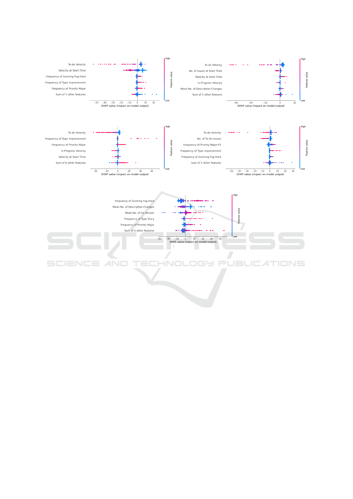
(a) Apache. (b) JBoss.
(c) Jira. (d) MongoDB.
(e) Spring.
Figure 1: Top five most important features per project, and how they influence predictions.
that improvement-type issues are often overestimated.
Similarly, when many major issues are included in the
iteration, the model predicts similar outcomes, possi-
bly reflecting a tendency for developers to overesti-
mate high-priority issues to allow some buffer in case
of unforeseen challenges. In-Progress Velocity has a
negative impact: a high volume of ongoing work by
prediction time tends to lower the expected vel
di f f
,
similar to the effect seen in Apache. Lastly, with re-
spect to Velocity at Start Time, low values do not af-
fect the prediction, but when a high number of story
points is planned at the start, the model predicts either
underperformance or overperformance. This suggests
a loss of predictability when large amounts of work
are committed upfront.
5.2.4 MongoDB
As in other projects, To-do Velocity is the most in-
fluential feature for MongoDB. The second key fea-
ture is the Number of To-Do Issues at prediction time;
when too many issues remain unstarted, this tends to
predict a lower vel
di f f
, which is reasonable. Simi-
lar to other projects, issues categorized as Improve-
ment or with a high priority (specifically Major-P3 in
the MongoDB project) also impact the model’s pre-
diction, suggesting that developers may overestimate
these types of issues here as well. Finally, we observe
that the Frequency of Gunning Fog Hard affects this
project as it does in Apache, with slightly higher ve-
locity predictions when issue descriptions are more
complex.
5.2.5 Spring
The Spring project stands out as the only project
where To-do Velocity is not among the top five fea-
tures. Here, the most influential feature is the Fre-
quency of Gunning Fog Hard. The impact of this fea-
ture is more pronounced compared to other projects:
issues with a low readability index (low Frequency of
Gunning Fog Hard) tend to predict a lower vel
di f f
,
whereas issues with higher readability index predict a
higher vel
di f f
. The second feature, Mean No. of De-
scription Changes, indicates that fewer changes in de-
scriptions correlate with higher predictions, perhaps
ENASE 2025 - 20th International Conference on Evaluation of Novel Approaches to Software Engineering
62

Table 5: Feature ranking across projects using Borda count,
and Bucket Pivot in brackets.
Feature Ranking
To-do Velocity 1 (1)
Frequency of Gunning Fog Hard 2 (2)
Frequency of Priority Major 3 (3)
Velocity at Start Time 4 (3)
In-Progress Velocity 5 (3)
Frequency of Type Improvement 6 (3)
No. of Issues at Start Time 7 (3)
Mean No. of Description Changes 8 (3)
Mean No. of Fix Version 9 (3)
No. of To-Do Issues 10 (3)
Frequency of Gunning Fog Easy 11 (3)
Frequency of Type Bug 12 (3)
Frequency of Type Documentation 13 (3)
Mean No. of Changing Fix Versions 14 (3)
No. of Issues In Progress 15 (3)
Frequency of Priority Major-P3 16 (3)
Frequency of Priority Critical 17 (3)
Mean No. of Comments 18 (3)
Frequency of Type Story 19 (3)
Frequency of Priority Blocker - P1 20 (3)
No. of Team Members 21 (3)
Variance No. of Changing Fix Versions 22 (3)
No. of Issues Removed 23 (3)
Added Velocity 24 (3)
Removed Velocity 25 (3)
Frequency of Type Task 26 (3)
Frequency of Priority Minor 27 (3)
suggesting that unclear issues could lead to underde-
livery. For the Mean No. of Fix Version (the number
of versions for which an issue was or will be fixed),
middle values have no predictive effect, while high
values are associated with higher vel
di f f
. Iterations in
this project that include many issues labeled as Story
or with the priority Major also show a tendency to
perform better than initially committed, potentially
because developers might overestimate these types of
issues.
5.2.6 Answer to RQ2
To find a consensus of the most influential features
across projects, we collect the mean absolute SHAP
values ranking for the top ten features of each project.
There are various approaches within the scope of
Rank Aggregation Problems for consolidating mul-
tiple rankings. The most traditional, known as the
Kemeny problem (Ali and Meil
˘
a, 2012), involves ag-
gregating a set of strict rankings (with no ties al-
lowed) to produce a consensus ranking that minimizes
the overall distance from the individual rankings be-
ing aggregated. Conversely, when ties are permit-
ted—indicating indifference between tied items—the
Optimal Bucket Order Problem (OBOP) is applied
(Aledo et al., 2017). In both cases, the input rankings
may be incomplete, as is the case here, where not all
features are ranked in every project.
In Table 5, we present the aggregated ranking
of features, using the Borda count method com-
bined with Bucket Order values in brackets. Features
ranked higher in each project accumulate more Borda
count points, resulting in a final score that represents
their overall influence across all projects. Addition-
ally, the Bucket Order values enhance this analysis
by grouping features into broader tiers where they are
considered equally ranked in importance. By assign-
ing Bucket Pivot values, we categorize features that
have close ranks across projects into the same bucket,
indicating an approximate level of influence rather
than an exact rank. This approach allows us to aggre-
gate incomplete rankings by summing up the points
assigned to each feature, creating a consolidated or-
der where the highest-scoring features appear at the
top of the list.
We observe that the top feature in the aggre-
gated ranking is To-do Velocity, which appears in four
projects. The second feature is Frequency of Gunning
Fog Hard, present in three projects, followed by the
remaining features in order according to the Bucket
Order.
The most important features that we observed in
the SHAP plots in Figure 1 can be grouped into cat-
egories that help us understand how they are related.
Table 6 summarizes the results for each project.
We observe that the starting status of the iteration
has a significant impact on the predicted vel
di f f
. The
number of issues at start time negatively impacts ve-
locity in one project. In contrast, Velocity at Start
Time shows negative effects in Apache and Jira but
has a positive effect in JBoss. Although the impor-
tance of this feature is evident, its influence is not con-
sistent across projects. One possible reason may be
the relative nature of SPs and the maturity of teams
in estimating issue complexity. Additionally, some
teams may allow new issues during their iterations,
while others do not.
Progress within the iteration is also a critical fac-
tor. Metrics related to the remaining workload con-
sistently appear across all projects. In four projects, a
high number of unstarted story points (To-do Veloc-
ity) predicts a lower vel
di f f
. It is reasonable to infer
that if much work remains unstarted, the iteration may
not be progressing as expected. Similar results appear
with No. of To-do Issues and In Progress Velocity.
Additionally, the clarity of requirements affects
delivery. A large proportion of issues with a high
Agile Effort Estimation Improved by Feature Selection and Model Explainability
63

Table 6: Top five most important features per project, grouped by feature category. (+) means positive effect on vel
di f f
, and
(-) means negative effect on vel
di f f
.
Feature Group Feature Apache JBoss Jira MongoDB Spring
Start of iteration status
Velocity at start time - + -
No. of issues at start time -
Iteration progress
To-do velocity - - - -
No. of To-do Issues -
In Progress Velocity - -
Clarity indicators
Mean No. of Description Changes + -
Frequency of Gunning Fog Hard + + +
Issue descriptors
Mean No. of Fix Version +
Freq. of priority Major + + + +
Freq. of type Story +
Freq. of type Improvement + + +
complexity in their descriptions predicts a better
vel
di f f
in the iteration in four projects. Furthermore,
a high number of changes to issue descriptions tends
to correlate with overdelivery.
Lastly, the type and priority of issues in an iter-
ation influence its outcome. These features are spe-
cific to each project, given that teams define their
own issue categories and priority levels. However,
we observe that a high count of issues marked as
Improvement or with a Major priority often results
in higher SHAP values, predicting a higher vel
di f f
in four projects. Other issue characteristics with a
smaller influence include the mean number of fix ver-
sions an issue affects and issues tagged as Story.
Answer to RQ2:
We find that features measuring the amount of
work at the start of an iteration significantly
impact predictions, though whether they af-
fect delivered velocity positively or negatively
varies across projects. Progress indicators
during the iteration also play an important
role in predictions: To-do velocity emerged as
significant in four out of five projects. Clar-
ity indicators, such as the Gunning Fog in-
dex for issue descriptions and the number of
changes made to descriptions, also influence
predictions. Lastly, there appears to be a pat-
tern with specific issue types, particularly pri-
ority Major or type Improvement, which tend
to be overestimated. Although categorization
varies by project, attention should be paid to
any emerging patterns in this regard.
5.3 Threats to Validity
Construct Validity. We address threats to construct
validity by utilizing real-world data from large open-
source projects provided by a prior study (Choetkier-
tikul et al., 2018). The target variable for predic-
tion, vel
di f f
, is measured in SPs. Although this unit
of measurement is commonly used in agile environ-
ments, it presents some challenges: SPs are relative
units that rely on human judgment, often achieved
through consensus, which may introduce bias into the
estimation process.
Conclusion Validity. We mitigate threats to conclu-
sion validity by employing a set of statistical tests
commonly found in the literature, ensuring a fair com-
parison of our model’s performance metrics. With re-
gards to the explainability techniques used, while we
can only speculate about the reasoning behind the se-
lected features and their impact on vel
di f f
, the use of
state-of-the-art interpretable models suggests that cer-
tain groups of features significantly influence iteration
performance.
Internal Validity. Regarding internal validity, we ac-
knowledge concerns raised in (Choetkiertikul et al.,
2018) related to preprocessing, handling of missing
data, and treatment of outliers within their datasets.
Their dataset extraction required imputing SP esti-
mates for 30% of issues that were not originally es-
timated, using the mean SPs from each project. Ad-
ditionally, they removed outliers in vel
di f f
and itera-
tions that had zero issues.
External Validity. To enhance external validity, we
used a large dataset encompassing five open-source
projects, which included 3,834 iterations and 56,687
issues. These projects vary in size and involve di-
verse development teams and issue management prac-
tices. However, despite the dataset’s size, it may
not represent all types of software projects. Indus-
trial projects might exhibit different behaviors, po-
ENASE 2025 - 20th International Conference on Evaluation of Novel Approaches to Software Engineering
64

tentially providing stronger insights into the common
features that should be considered when estimating
velocity. Therefore, further research with additional
datasets from industrial projects is necessary to deter-
mine whether our findings are also applicable in an
industrial context.
6 CONCLUSION
Agile methodologies are widely applied, being one of
the most adopted practices the iterative development.
In this work, we have proposed the use of feature sub-
set selection to reduce the complexity of the machine
learning models often used in the literature to predict
software effort estimation. We have statistically tested
that reducing the feature subset to 10% of its orig-
inal size can be done without incrementing the ob-
tained error measures. With a minimal subset of fea-
tures, we have applied state-of-art global explanabil-
ity methods. Specifically, we made use of SHAP val-
ues to analyze the topmost important features that in-
fluence the difference between the committed and the
actual velocity of an iteration. We find out that there
are common features that appear in multiple projects,
which can be grouped into categories that help us un-
derstand their effects on the predicted velocity.
In future works, we plan to expand this study with
datasets from industrial projects, to assess whether
our findings can be extended to wider contexts. Fur-
thermore, it might be interesting to explore the effect
on vel
di f f
through the interaction of two or more fea-
tures, rather than considering only univariate effects.
ACKNOWLEDGEMENTS
This work has been partially funded by the
Government of Castilla-La Mancha and “ERDF
A way of making Europe” under project SB-
PLY/21/180225/000062 and by the Universidad de
Castilla-La Mancha and “ERDF A Way of Making
Europe” under project 2022-GRIN-34437.
REFERENCES
Abadeer, M. and Sabetzadeh, M. (2021). Machine learning-
based estimation of story points in agile development:
Industrial experience and lessons learned. In 2021
IEEE 29th International Requirements Engineering
Conference Workshops (REW), pages 106–115.
Abrahamsson, P., Fronza, I., Moser, R., Vlasenko, J., and
Pedrycz, W. (2011). Predicting development effort
from user stories. 2011 International Symposium on
Empirical Software Engineering and Measurement,
pages 400–403.
Abrahamsson, P., Moser, R., Pedrycz, W., Sillitti, A.,
and Succi, G. (2007). Effort prediction in iterative
software development processes – incremental versus
global prediction models. In First International Sym-
posium on Empirical Software Engineering and Mea-
surement (ESEM 2007), pages 344–353.
Aledo, J. A., G
´
amez, J. A., and Rosete, A. (2017). Utopia
in the solution of the bucket order problem. Decision
Support Systems, 97:69–80.
Ali, A. and Meil
˘
a, M. (2012). Experiments with kemeny
ranking: What works when? Mathematical Social
Sciences, 64(1):28–40. Computational Foundations of
Social Choice.
Alsaadi, B. and Saeedi, K. (2022). Data-driven effort esti-
mation techniques of agile user stories: a systematic
literature review, volume 55. Springer Netherlands.
Anderson, D. (2010). Kanban: Successful Evolutionary
Change for Your Technology Business. Blue Hole
Press.
Arcuri, A. and Briand, L. (2014). A hitchhiker’s guide to
statistical tests for assessing randomized algorithms in
software engineering. Software Testing, Verification
and Reliability, 24(3):219–250.
Bermejo, P., De La Ossa, L., and Puerta, J. M. (2011).
Global feature subset selection on high-dimensional
datasets using re-ranking-based edas. In Proceedings
of the 14th International Conference on Advances in
Artificial Intelligence: Spanish Association for Artifi-
cial Intelligence, page 54–63. Springer-Verlag.
Bhattacharya, P. and Neamtiu, I. (2011). Bug-fix time pre-
diction models: can we do better? In Proceedings
of the 8th Working Conference on Mining Software
Repositories, MSR ’11, page 207–210, New York,
NY, USA. Association for Computing Machinery.
Choetkiertikul, M., Dam, H. K., Tran, T., Ghose, A., and
Grundy, J. (2018). Predicting delivery capability in
iterative software development. IEEE Transactions on
Software Engineering, 44:551–573.
Choetkiertikul, M., Dam, H. K., Tran, T., Pham, T., Ghose,
A., and Menzies, T. (2019). A deep learning model for
estimating story points. IEEE Transactions on Soft-
ware Engineering, 45:637–656.
Cohn, M. (2004). User Stories Applied: For Agile Software
Development. Addison Wesley Longman Publishing
Co., Inc., USA.
Cohn, M. (2005). Agile Estimating and Planning. Prentice
Hall PTR, USA.
Digital.ai (2023). The 17th state of agile report.
Fu, M. and Tantithamthavorn, C. (2023). Gpt2sp: A
transformer-based agile story point estimation ap-
proach. IEEE Transactions on Software Engineering,
49(2):611–625.
Guyon, I. and Elisseeff, A. (2003). An introduction to
variable and feature selection. J. Mach. Learn. Res.,
3(null):1157–1182.
Hearty, P., Fenton, N., Marquez, D., and Neil, M. (2009).
Predicting project velocity in xp using a learning dy-
Agile Effort Estimation Improved by Feature Selection and Model Explainability
65

namic bayesian network model. Software Engineer-
ing, IEEE Transactions on, 35:124 – 137.
Kocaguneli, E., Menzies, T., and Keung, J. W. (2012). On
the value of ensemble effort estimation. IEEE Trans-
actions on Software Engineering, 38(6):1403–1416.
Langdon, W. B., Dolado, J., Sarro, F., and Harman, M.
(2016). Exact mean absolute error of baseline pre-
dictor, marp0. Information and Software Technology,
73:16–18.
Lundberg, S. M. and Lee, S.-I. (2017). A unified ap-
proach to interpreting model predictions. In Guyon,
I., Luxburg, U. V., Bengio, S., Wallach, H., Fer-
gus, R., Vishwanathan, S., and Garnett, R., editors,
Advances in Neural Information Processing Systems,
volume 30. Curran Associates, Inc.
Malgonde, O. and Chari, K. (2019). An ensemble-based
model for predicting agile software development ef-
fort, volume 24.
Mendes, E. (2010). Chapter 5 - an overview of web ef-
fort estimation. In Advances in Computers: Improving
the Web, volume 78 of Advances in Computers, pages
223–270. Elsevier.
Mockus, A., Weiss, D., and Zhang, P. (2003). Understand-
ing and predicting effort in software projects. Pro-
ceedings - International Conference on Software En-
gineering.
Panjer, L. D. (2007). Predicting eclipse bug lifetimes. In
Fourth International Workshop on Mining Software
Repositories (MSR’07:ICSE Workshops 2007), pages
29–29.
Porru, S., Murgia, A., Demeyer, S., Marchesi, M., and
Tonelli, R. (2016). Estimating story points from issue
reports. In Proceedings of the The 12th International
Conference on Predictive Models and Data Analytics
in Software Engineering, PROMISE 2016, New York,
NY, USA. Association for Computing Machinery.
Ribeiro, M. T., Singh, S., and Guestrin, C. (2016). ”why
should i trust you?”: Explaining the predictions of any
classifier. In Proceedings of the 22nd ACM SIGKDD
International Conference on Knowledge Discovery
and Data Mining, KDD ’16, page 1135–1144, New
York, NY, USA. Association for Computing Machin-
ery.
Sarro, F., Petrozziello, A., and Harman, M. (2016a). Multi-
objective software effort estimation. In Proceedings
of the 38th International Conference on Software En-
gineering, ICSE ’16, page 619–630, New York, NY,
USA. Association for Computing Machinery.
Sarro, F., Petrozziello, A., and Harman, M. (2016b). Multi-
objective software effort estimation. In Proceedings
of the 38th International Conference on Software En-
gineering, ICSE ’16, page 619–630, New York, NY,
USA. Association for Computing Machinery.
Scott, E. and Pfahl, D. (2018). Using developers’ features to
estimate story points. In Proceedings of the 2018 In-
ternational Conference on Software and System Pro-
cess, ICSSP ’18, page 106–110, New York, NY, USA.
Association for Computing Machinery.
Shepperd, M. and MacDonell, S. (2012). Evaluating predic-
tion systems in software project estimation. Informa-
tion and Software Technology, 54(8):820–827. Spe-
cial Issue: Voice of the Editorial Board.
Tawosi, V., Moussa, R., and Sarro, F. (2023). Agile effort
estimation: Have we solved the problem yet? insights
from a replication study. IEEE Transactions on Soft-
ware Engineering, 49:2677–2697.
Trendowicz, A. and Jeffery, R. (2014). Software Project
Effort Estimation. Springer, Berlin.
ENASE 2025 - 20th International Conference on Evaluation of Novel Approaches to Software Engineering
66