Optimizing Truck Flow in Ship Unloading: A Real-Time Simulation

Approach for the Port of Itaqui

Carlos Eduardo V. Gomes

, Victor Jos

e B. A. Martinez

, Jo

ao Augusto F. N. de Carvalho

Francisco Glaubos Nunes Cl

ımaco

, Geraldo Braz J

unior

, Tiago Bonini Borchatt

and Jo

ao Dallyson Sousa de Almeida

ucleo de Computac

ao Aplicada, Universidade Federal do Maranh

ao (UFMA), S

ao Lu

ıs, MA, Brazil

{carlos.evg, victor.martinez, augusto.joao}@discente.ufma.br,

{fra a.br

Keywords:

Truck Congestion, Port Operation, Operational Efﬁciency, Real-Time Discrete Simulation.

Abstract:

Truck congestion in port yards is a signiﬁcant issue that impacts the operational efﬁciency and competitive-

ness of port terminals. This study examines the logistics ﬂow dynamics in the ship unloading area of the

Port of Itaqui. Through modeling and simulation methodologies, it aims to identify bottlenecks and optimize

operations. We collected and analyzed port data to establish simulation parameters, which were categorized

into various groups, including system administration, truck ﬂows, and required resources. Based on the con-

ceptual modeling of truck and ship movements, we developed a simulation system that visualizes the effects

of different operational decisions. The results of the simulation are crucial for identifying critical points and

formulating strategies to reduce congestion.

1 INTRODUCTION

The unloading operations of bulk products in ports

represent a fundamental step in the global logistics

and distribution of goods. These products, including

grains, minerals, coal, and liquids, are transported in

large quantities and require specialized infrastructure

and procedures to be unloaded efﬁciently and safely.

The efﬁciency of these operations is crucial, as delays

can result in increased costs, congestion, and a nega-

tive impact on the supply chain (Du et al., 2023).

One of the main challenges in these operations

is balancing unloading speed with operational safety.

Due to the large volume of material to be handled, the

risk of accidents and environmental damage is signif-

icant. Moreover, the variability in the characteristics

of bulk products, such as density and particle size, can

directly impact the efﬁciency of unloading equipment

and the stability of port structures (de Le

on et al.,

https://orcid.org/0009-0007-0273-4373

https://orcid.org/0009-0001-8759-8927

https://orcid.org/0009-0004-1165-1228

https://orcid.org/0000-0002-1357-1318

https://orcid.org/0000-0003-3731-6431

https://orcid.org/0000-0002-3709-8385

https://orcid.org/0000-0001-7013-9700

2021).

Another critical aspect is the optimization of oper-

ational costs. The maintenance of equipment, work-

force training, and management of operation times

directly inﬂuence the total costs of port operations.

Therefore, ﬁnding the ideal balance between efﬁ-

ciency, safety, and cost is a constant challenge for port

operators.

The Port of Itaqui, in the state of Maranh

ao (see

1), known for handling solid and liquid bulk, stands

out for its deep waters, rail connections, and struc-

tured terminals, providing competitive logistics for its

clients. Historically, the port has focused on grain

exports, especially soybeans and corn, and receiving

petroleum products such as diesel, gasoline, and fer-

tilizers. In 2022, Itaqui reached its highest cargo vol-

ume in history, handling 33.61 million tons, with solid

bulk accounting for 23 million tons, a 19% increase

over the previous year. In 2023, for the ﬁrst time, the

port registered the handling of 2 million tons of soy-

beans in a single month, consolidating its position as

the 4th largest public port in Brazil, according to the

2023 Aquatic Performance Report released by AN-

TAQ (National Agency for Waterway Transportation

(ANTAQ), 2024).

This study aims to address key operational chal-

lenges at the Port of Itaqui by identifying bottlenecks

444

Gomes, C. E. V., Martinez, V. J. B. A., N. de Carvalho, J. A. F., Clímaco, F. G. N., Braz Júnior, G., Borchatt, T. B. and Sousa de Almeida, J. D.

Optimizing Truck Flow in Ship Unloading: A Real-Time Simulation Approach for the Port of Itaqui.

DOI: 10.5220/0013232800003929

Paper published under CC license (CC BY-NC-ND 4.0)

In Proceedings of the 27th International Conference on Enterprise Information Systems (ICEIS 2025) - Volume 1, pages 444-455

ISBN: 978-989-758-749-8; ISSN: 2184-4992

Figure 1: Port of Itaqui, on the west coast of the island

ao Marcos Bay), 11 km from S

ao Lu

ıs (EMAP - Empresa

Maranhense de Administrac¸

ao Portu

aria, 2024).

in truck ﬂow, both within the port’s infrastructure and

at external logistical support points. It also seeks to

clarify the relationship between truck volume in the

primary operational area and the ship discharge rate,

offering a detailed understanding of how many trucks

are needed to efﬁciently meet active contracts. These

insights are crucial for optimizing resource allocation

and streamlining port operations.

Directly observing dynamics in the physical port

environment poses signiﬁcant challenges due to spa-

tial and logistical constraints. To overcome these

limitations and gain a comprehensive understanding

of how each component affects port operations, this

study has developed an innovative real-time simula-

tion system. The main contribution of this simulator

is allows for a detailed examination of the current port

conditions and serves as a dynamic platform to test

the effects of variable adjustments on truck ﬂow, ship

discharge efﬁciency, and overall port activity. More-

over, with this system, it becomes possible to create

data-driven strategies that address operational inefﬁ-

ciencies, thereby enhancing both the throughput and

resilience of the Port of Itaqui’s logistics framework.

The rest of the article is structured as follows: Sec-

tion 2 presents the theoretical framework necessary

for understanding the work developed; Section 3 de-

tails the methodological procedures used for the de-

velopment of the simulator; Section 4 provides the

description of the simulated scenarios and the analysis

of the results obtained; and ﬁnally, Section 5 presents

the conclusions and possibilities for future work.

2 RELATED WORK

There are several causes for truck congestion in ports.

Many ports face space constraints, limiting their abil-

ity to efﬁciently handle large volumes of trucks. This

problem is exacerbated by the growth of the interna-

tional market, which increases the demand for port

services beyond the available capacity (Napitupulu

et al., 2022).

Bulk cargo unloading operations at ports are es-

sential components of the supply chain, directly af-

fecting the efﬁciency and effectiveness of logistics

operations. These activities involve complex inter-

actions between various elements, such as schedul-

ing, coordination, and cargo handling. To understand

the main concepts involved and their impact on sup-

ply chain efﬁciency, we can analyze the following as-

pects:

Truck Appointment Systems (TAS): Implement-

ing TAS in port terminals can signiﬁcantly increase

yard efﬁciency, reduce congestion, and balance de-

mand with available capacity. This system helps min-

imize truck wait times and container handling, essen-

tial factors for maintaining smooth operations at the

port’s land interface (Wang et al., 2023). TAS allows

for better distribution of trucks throughout the day,

optimizing infrastructure use and reducing unneces-

sary queues, resulting in more efﬁcient operations.

Train Scheduling: In ports specializing in bulk

cargo, train scheduling for unloading is a complex

task due to uncertainties in processing times. Effec-

tive scheduling, whether deterministic or stochastic,

is essential to ensure deadlines are met, and cargo

transfer to warehouses occurs in a timely manner.

Techniques such as mixed integer programming, con-

straint programming, and greedy randomized algo-

rithms are commonly used to optimize these opera-

tions (Menezes et al., 2016).

Disruption Management: Bulk cargo operations

often face disruptions, making effective uncertainty

management essential. Frequent rescheduling and en-

hanced dispatching rules can mitigate the deteriora-

tion of operational performance, ensuring adherence

to schedules and consequently increasing overall efﬁ-

ciency (Menezes et al., 2016). The ability to quickly

adjust the schedule in the face of unexpected events is

a determining factor in avoiding delays and minimiz-

ing operational impacts.

Port operations, especially those related to the un-

loading of bulk products, face signiﬁcant challenges

due to truck congestion. To analyze and mitigate this

problem, many authors explore modeling and simu-

lation approaches widely used to optimize truck ﬂow

and minimize delays. Among the most common ap-

proaches are discrete event simulation models, which

allow the replication of port operations in virtual sce-

narios, simulating the impact of different operational

variables, such as truck ﬂow, unloading times, and in-

frastructure bottlenecks (Iannone et al., 2016). Ad-

Optimizing Truck Flow in Ship Unloading: A Real-Time Simulation Approach for the Port of Itaqui

445

ditionally, agent-based modeling (ABM) techniques

have been used to model the interactions between

trucks, port operators, and available resources, con-

sidering behavioral variability and uncertainties in op-

erations (Uthpala et al., 2023). Stochastic optimiza-

tion models and linear programming also appear in

the literature to solve allocation and scheduling prob-

lems, aiming to minimize waiting times and conges-

tion.

The Port of Los Angeles successfully imple-

mented PierPass, a program that shifts part of port

operations to off-peak hours, signiﬁcantly reducing

daytime congestion. Another successful case was the

use of Truck Appointment Systems (TAS) at the Port

of Hamburg, Germany, where optimized truck arrival

coordination managed to balance port capacity with

demand, improving efﬁciency and truck ﬂow (Notte-

boom et al., 2022). However, there are also failures

in congestion management. At the Port of Santos,

Brazil, the implementation of ﬂow control technolo-

gies was insufﬁcient due to the lack of proper integra-

tion with operations outside the port, resulting in long

truck queues and delays, demonstrating that the effec-

tiveness of solutions like TAS depends on expanded

infrastructure and coordination policies (Hilsdorf and

Nogueira Neto, 2015).

Although modeling and simulation have provided

advances in understanding truck ﬂow, there are still

opportunities to better explore integrating intelligent

logistics systems, such as new approaches and strate-

gies to more proactively predict and mitigate conges-

tion. Moreover, most studies focus on large-scale

ports, leaving a gap concerning the application of

these solutions in medium and small ports, which of-

ten do not have the same technological resources or ﬁ-

nancial capacity to implement advanced management

solutions.

3 METHODOLOGY

The methodology applied in this work consists of

multiple steps, including the deﬁnition of the object

studied and its problems, the analysis of port data, and

the development of a simulation system (see Figure

2). The system covers not only the conceptual models

but also its computational applications. Each step is

detailed in the following sections.

3.1 Object of Study and Its Problems

Meetings were held with managers and operators, and

technical on-site visits were to understand the differ-

ent scenarios characterizing the logistical and opera-

Methodology

Understanding the study

object and its problems

Simulation system development

Port data analysis Parameters definition

Definition of simulation

models

Figure 2: Methodology diagram.

tional ﬂow in the ship unloading area at the Port of

Itaqui. These interactions provided a deeper insight

into the cyclical activities of the trucks, the stages of

the port ﬂow, the role of operators in the port’s pri-

mary area, and the importance of equipment such as

scales and scanners to maintain the efﬁcient ﬂow of

trucks.

Based on these observations, the following key

concepts are deﬁned for the operability of port activi-

ties:

• Truck Flow (carousel). Refers to the cycli-

cal movement of trucks between the different

phases of unloading products from ships and sub-

sequently delivering them to customers. This ﬂow

is essential to maintain the pace of port operations

and prevent bottlenecks.

• Window. This refers to a registry system at the

Port associated with a contract. Each window is

linked to a speciﬁc ship, a product type, a client,

and the number of trucks involved in transporta-

tion.

• Pull. This is the authorization granted to a truck

to leave the “logistical support area” and proceed

to the remaining stages of the ﬂow process within

the port.

Based on these concepts, it can be said that con-

trolling the truck ﬂow at the port is essentially control-

ling the ﬂow of trucks for each window in operation.

This control is carried out by port operators, who use

two key parameters to manage the pull:

• Initial Pull. A manually deﬁned parameter speci-

fying the number of trucks that should be between

the stages of “Access Gate Entry” and the “Collec-

tion Point” (quay area) for each window

• Blocking Pull. Also manually deﬁned, this pa-

rameter sets the maximum limit of trucks between

the stages of “Access Gate Entry” and “Access

Gate Exit” for each window.

To identify the inﬂuences of controlling the ﬂows

of each window and the various impacts that pull pa-

rameters have across the Port, data analysis has be-

gun.

ICEIS 2025 - 27th International Conference on Enterprise Information Systems

446

3.2 Analysis of Port Data

Data collection and analysis of the operational pro-

cesses at the Port of Itaqui were performed to conduct

an accurate simulation. These analyses included the

following aspects:

• Average Time of Truck Stages in the Flow.

Analysis of the average times trucks spend in each

process phase, from entry to exit, including un-

loading time and internal movements.

• Number of Trucks at each Stage of the Flow.

Evaluation of the number of trucks moving be-

tween the different stages of the port process, aim-

ing to understand how truck density affects oper-

ational performance.

• Analysis of the Pulls Performed by Operators.

Study of operator behavior regarding pull control,

identifying patterns and impacts on the smooth-

ness of truck ﬂow.

Based on these analyses, simulation control pa-

rameters were deﬁned to manage the behavioral and

technical aspects of the simulated scenarios. These

parameters were organized into ten groups: conﬁg-

uration, existence, truck ﬂows, timing, delays, load,

resources, pull, and context. Each group encom-

passes speciﬁc elements that reﬂect real-world op-

erational conditions in the port sector, including the

movement and handling of trucks, allocation of crit-

ical resources, and management of delays and load

weights. After deﬁning the simulator input param-

eters and identifying the aspects to be implemented

and observed, conceptual models were developed to

represent the operations of these components.

3.3 Simulation Models

The simulation model was structured in four great

ﬂows: trucks’ ﬂow, ships’ ﬂow, pulls, and simula-

tion, besides auxiliary managers of resources, win-

dows, and operators.

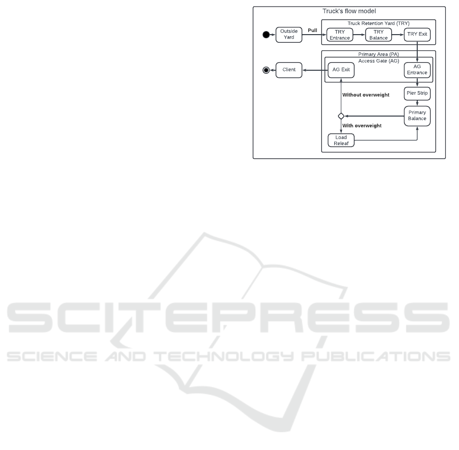
3.3.1 Trucks’ Flow Model

The model shown in Figure 3 is the primary reference

for understanding the simulator’s behavior. It helps

identify potential bottlenecks at each ship’s unloading

process stage. The key steps in this ﬂow are:

• External Yard. This is where trucks wait to be

pulled to begin their activities. It is also the place

where trucks return to start a new cycle after de-

livering products to the client;

• Truck Retention Yard (TRY). After being

pulled, this is where trucks go to be weighed on

Truck Retention Yard (TRY)

Primary Area (PA)

Access Gate (AG)

Truck's flow model

Outside

Yard

Client

Entrance

TRY

Entrance

TRY

Balance

TRY Exit

Pull

AG Exit

Pier Strip

Primary

Balance

Load

Releaf

With overweight

Without overweight

Figure 3: Trucks’ ﬂow model.

the TRY scale. This stage is important for the

subsequent weighing of the trucks loaded with the

products from the ships;

• Primary Area:

– Access Gate (GA). A checkpoint responsible

for identifying trucks entering and exiting the

primary area;

– Quay Strip. The location where the grabbing

cranes are situated, where the trucks are loaded

with products from the ships;

– Primary Scale. Weighing of the truck to iden-

tify overweight loads;

– Load Relief. The location where trucks ofﬂoad

excess weight that exceeds the truck’s capacity;

• Client. This is the stage where the products col-

lected from the port trucks are delivered to the

contracting clients.

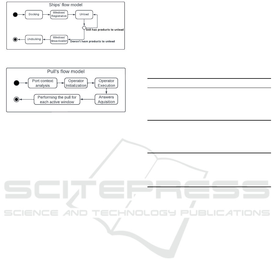
3.3.2 Ships’ Flow Model

Next, the ship ﬂow model was developed, as shown

in ﬁgure 4. This model is essential for simulating

sufﬁciently long periods, allowing the arrival and de-

parture of ships from the port docks. The interaction

between the ship and truck ﬂows is crucial, as it di-

rectly inﬂuences the port’s capacity to handle large

cargo volumes efﬁciently. The main stages of the ship

activity cycle are presented in this model:

• Docking and Undocking. When the ship arrives

and departs from the port. It is important to in-

troduce new products into the simulation so that

operations do not cease;

• Window Registration. This involves registering

contracts for each product, ship, and customer in

the simulation. This step is essential to deﬁne

new windows and allow new operations within the

port;

Optimizing Truck Flow in Ship Unloading: A Real-Time Simulation Approach for the Port of Itaqui

447

Ships' flow model

Docking

Undocking

Windows'

Registration

Windows'

desactivation

Unload

Still has products to unload

Doesn't have products to unload

Figure 4: Ships’ ﬂow model.

Pull's flow model

Port context

analysis

Performing the pull for

each active window

Operator

Initialization

Operator

Execution

Answers

Aquisition

Figure 5: Pull’s ﬂow model.

• Unloading. The stage where trucks unload prod-

ucts from the ships while they are docked;

• Window Deactivation. After all the products

from the ship are unloaded, all its windows are

deactivated, and the undocking process begins.

3.3.3 Pulls’ Flow Model and Operators Manager

To properly deﬁne and execute port activities through

pull control, a model reﬂecting the pull execution ﬂow

was developed, as shown in ﬁgure 5. This model is

essential as it outlines the steps in activating the port’s

operations. By using this model, it becomes easier to

deﬁne the methodology for setting parameters, such

as the initial pull and block pull, which are determined

by the operator. Below are the main stages of the pull

activity ﬂow:

• Port Context Analysis. At this stage, the simula-

tor compiles data related to the presence of trucks

in the primary area and delivers it to the operator;

• Operator Initialization. The stage where the

method to be used for executing the pull is de-

ﬁned;

• Operator Execution. The operator performs cal-

culations based on the current port context to de-

termine the pull values;

• Response Acquisition. At this stage, the simula-

tor converts the values deﬁned by the operator into

the parameters “initial pull” and “block pull”;

• Pull Execution for Each Active Window. The

pull is then properly executed, pulling the trucks

for each active window at that moment.

Two operation models were also developed to de-

ﬁne the pull methodology. The ﬁrst model, titled

“guided pull,” presented in Table 1, deﬁnes a guide

for the initial pull and block pull parameters based on

analyzing actual pull data performed at the port. This

model determines predeﬁned values for the parame-

ters “initial pull” and “block pull” according to the

number of docked ships in operation and the number

of windows open simultaneously per ship. These val-

ues were empirically deﬁned by professionals work-

ing at the Itaqui port.

Table 1: Operation model for a port-driven pull system.

Ships Open windows Initial pull Blocking pull

1 15 60

2 9 30

3 6 20

4 5 15

5 5 12

1 15 30

2 6 15

3 5 10

4 5 8

5 3 6

1 8 20

2 6 10

3 5 7

4 5 5

5 3 4

The second model, titled “minimum pull,” always

performs the smallest possible pull that guarantees the

correct execution of port operations. This model re-

lies on two input parameters: “minimum queue size at

the dockside” and “maximum queue size at the dock-

side.” The queue at the dockside deﬁnes the num-

ber of trucks that are either using a collector, waiting

for one, or moving towards one. Thus, the model al-

ways tries to pull the smallest possible value within

the range deﬁned by these parameters.

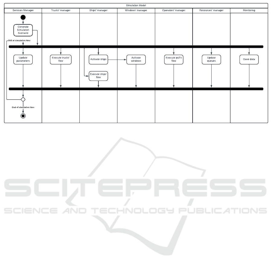
3.3.4 Simulation’s Flow Model

The simulation ﬂow, presented in Figure 6, was cre-

ated from the truck and ship ﬂow models and the re-

source and window managers. This ﬂow integrates all

the system’s elements, allowing for a holistic analysis

of port operations. It enables the simulation of various

scenarios, including changes in the number of ships,

types of cargo, truck availability, and operational con-

ditions. The simulation model encompasses six main

managers:

• Service Manager. Controls all services and other

managers. In addition to initializing each man-

ager’s operation, it manages the creation of clients

for the simulation, updates the simulation pa-

rameters throughout its execution, controls the

ICEIS 2025 - 27th International Conference on Enterprise Information Systems

448

Simulation Model

Services Manager Trucks' manager Ships' manager Windows' manager Operators' manager Resources' manager Monitoring

Activate

windows

Activate ships

Execute trucks'

flow

Save data

Execute ships'

flow

Update

parameters

Update

queues

Still at simulation time

End of simulation time

Execute pull's

flow

Generate

Simulation

Scenario

Figure 6: Simulation model.

simulation time, and ensures the program con-

cludes once the maximum duration of operations

is reached.

• Truck Manager. Responsible for ensuring that

each truck follows the ﬂow presented in ﬁgure 3

correctly, as well as generating and activating new

trucks when necessary.

• Ship Manager. Responsible for executing the

ﬂow of each ship throughout the simulation and

managing its products.

• Window Manager. Controls and deﬁnes which

windows enter and exit activity.

• Operator Manager. Responsible for executing

the pulls throughout the simulation based on the

operator modeling described in Section 3.3.

• Resource Manager. Controls the use of scales,

gates, and collectors throughout the operation and

is crucial for sending messages for their monitor-

ing.

Monitoring. Responsible for observing the sim-

ulation and storing the state of each truck, ship, re-

source, and port region. It is essential to save the

simulation results, provide important data to all other

managers, and ensure smooth operations.

The simulation model comprises two main activ-

ity groups: the ﬁrst is the initialization of the simu-

lation context, in which all managers start their pro-

cesses, and the second is the simulation execution,

where all managers perform their activities in paral-

lel within a loop as long as the simulation time has

not ﬁnished.

3.4 Simulation System Development

The simulation models for the Port of Itaqui were im-

plemented using SimPy (Simpy, 2024), a Python li-

brary designed for discrete-event simulation. Each

main model—truck ﬂow, ship ﬂow, and resource man-

agement—was structured as a separate process within

SimPy. The truck ﬂow model simulates the move-

ment of trucks through various stages, such as wait-

ing in the external yard, weighing, and cargo collec-

tion at the dock. Resources like scales and collection

points were modeled using SimPy’s Resource class,

ensuring that multiple trucks or ships can interact with

these limited resources realistically. The simulation

uses Python generator functions to manage parallel

activities, allowing trucks, ships, and other entities

to progress simultaneously through their respective

stages. SimPy’s real-time event scheduling enables

precise control over these operations, adhering to con-

straints like waiting times and resource availability.

Additionally, veriﬁcation and validation routines

were implemented to ensure model accuracy. This in-

cluded comparing the simulation results with histori-

cal data from the Port of Itaqui and conducting sensi-

tivity tests to understand how changes in key parame-

ters impact system performance.

The resulting simulation system allows for the

analysis of port operation ﬂows and provides a plat-

form to test interventions that can improve efﬁciency,

reduce congestion, and optimize resource manage-

ment at the port.

Optimizing Truck Flow in Ship Unloading: A Real-Time Simulation Approach for the Port of Itaqui

449

4 RESULTS AND DISCUSSION

In this section, the results obtained from the simula-

tion of the pre-determined scenarios will be presented

and discussed. The main objective is to evaluate the

impact of the controlled variables on truck ﬂow and

identify potential bottlenecks in port operations. The

simulation was structured to test various parameters,

such as event timing, pull control, and resource ca-

pacity, considering different operational conditions.

Each simulation generates, as its ﬁnal result, a

multi-page spreadsheet that covers various aspects of

port logistics. The spreadsheet was built based on the

simulation models and presents the following infor-

mation:

• Truck Flows. Contains the complete history of

truck ﬂows within the port, covering each step

taken by each truck. It also tracks all stages of the

logistical process, including weightings, entries,

and exits from speciﬁc port areas;

• Pulls. Lists the number of trucks pulled within

time windows, relating them to the ship, client,

and product. It also provides information on the

“initial pull” and “blocking pull” parameters ap-

plied by the operator, as well as the status of trucks

in the unloading areas;

• Delays. Records truck delays at different stages

of the carousel;

• Trucks per Area. Monitors the number of trucks

in each area throughout the truck ﬂow;

• Trucks per Ship. Displays the distribution of

trucks by ship in the primary area and overall port

ﬂow;

• Scales, Access Gates, and Scanners. Details the

queue waiting time and processing time in the

main operational areas of the port.

The simulator has important base conﬁgurations

that are valid for executing all simulation scenarios

presented in section 4.1. These include the total sim-

ulation duration—conﬁgured for 48 hours, the base

time unit, i.e., the discrete-time interval advanced at

each step of the simulator—set to 1 minute, the num-

ber of clients and trucks per client—conﬁgured to 4

and 30, respectively, the number of ships docked at

the same time, the number of products loaded by each

ship, and the number of active windows per docked

ship—conﬁgured to 1, 2, and 5, respectively. Finally,

the base conﬁguration for port resources includes de-

termining the number of scales in the Truck Retention

Yard (TRY) and the Primary Area (AP), both of which

are set to 2. Additionally, the number of grab cranes

per ship is set to 1. This conﬁguration is parameter-

ized and serves as a common context for various sim-

ulation scenarios.

4.1 Discussion Analysis of Simulation

Scenarios

To analyze the behavior of truck ﬂow in the port area,

a systematic variation of 8 parameters was proposed:

• Availability of trucks to be pulled;

• Number of docked ships;

• Number of active windows per docked ship;

• Availability of scales along the port ﬂow;

• Availability of grab cranes;

• Minimum percentage of truck overload;

• Minimum percentage of truck delays for each

stage of the ﬂow;

• Minimum and maximum limits for pulls in the

minimum pull model.

The following results are from different simu-

lation scenarios executed on an Intel® Core™ i7-

12700F computer with 32 GiB of RAM. For each

variation, it is important to observe and understand

how each one affects the duration of truck ﬂows, the

unloading rate of products from each ship, and the

presence of bottlenecks throughout the carousel.

4.1.1 Number of Ships Docked and Active

Windows per Ship

As presented in the conceptual model, the guided pull

model depends on the number of ships docked and ac-

tive windows per ship. Thus, to validate the inﬂuence

of this model, the parameters for the number of ships

docked in the port and the number of open windows

simultaneously per ship vary from 1 to 3 and from 1 to

5, respectively. The simulations produced the results

presented in this section from the variation of these

parameters.

Figures 7, 8, and 9 display the average number

of trucks in the primary area and its respective sub-

regions over the entire simulation period, which was

divided into 10-minute intervals. This data corre-

sponds to scenarios with one, two, and three ships

docked at the port. This allows for a clear observa-

tion of how guided pull affects port activities.

In all three ﬁgures, seasonality is evident, charac-

terized by smaller peaks and valleys throughout the

operations. This pattern arises from the cyclical na-

ture of truck and ship movements, which occur peri-

odically. The primary factor contributing to this peri-

odicity is the pull operation, which activates groups of

ICEIS 2025 - 27th International Conference on Enterprise Information Systems

450

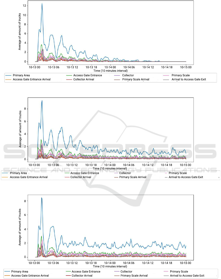
Figure 7: Average of the amount of trucks per region through time for 1 ship.

Figure 8: Average of the amount of trucks per region through time for 2 ships.

Figure 9: Average of the amount of trucks per region through time for 3 ships.

Optimizing Truck Flow in Ship Unloading: A Real-Time Simulation Approach for the Port of Itaqui

451

Figure 10: Average of the queues’ size per resource through time for 3 ships.

trucks. These trucks move together in a coordinated

manner through the carousel, creating a “burst” effect

in their movement.

At the beginning of operations, many trucks are

concentrated in the primary area. However, by the end

of the process, there are few or no trucks remaining.

This change occurs due to the ﬂow of ships; once they

deliver their cargo, they depart the port to make space

for incoming ships. As a result, there is a temporary

decrease in port activities.

In Figure 7, we observe the behavior of port oper-

ations when only one ship can dock at a time, high-

lighting the variation in the number of active win-

dows available simultaneously. Towards the end of

the graph, it becomes evident that no more trucks are

in the primary area, as all windows have been ﬁlled.

This indicates that no additional products will be de-

livered, leading the ship to leave the port and result-

ing in a prolonged period of idleness. This situation is

undesirable because it not only limits service to a few

ships at a time but also extends the waiting period for

the arrival of new ships. Consequently, this increases

overall operational costs by delaying service to ves-

sels and the delivery of products to customers.

Figures 8 and 9 illustrate the port regions when

two and three ships are docked, respectively. In both

scenarios, the operations remain active throughout the

simulation period. This suggests that even when all

tasks for a ship are completed, there is only a tempo-

rary reduction in activities, which is clearly evident in

Figure 8 and more subtly in Figure 9. The key take-

away is that the port is better equipped to meet cus-

tomer demands and maintain continuous operations

when multiple ships are docked simultaneously.

In all the scenarios presented, it is evident that

no sub-region within the primary area reaches four

trucks. This suggests no signiﬁcant bottlenecks in

these port areas for the scenarios examined. The

queues’ sizes for each port resource were analyzed to

assess potential congestion in the port regions. Figure

10 illustrates the average queue size over the simu-

lation period, recorded every minute, for each scale,

gate, and collector present in the port during the sce-

nario with three ships docked.

Among the presented resources, the scales in the

truck retention yard are the only ones that show a

larger queue size, indicating a bottleneck point that

can be observed. The other resources present in the

primary area align with the behavior presented in Fig-

ures 7, 8, and 9, as they do not show considerable

queues. Thus, it becomes evident to identify idleness

and congestion in port activities through the simula-

tion and variation of the number of docked ships and

active windows.

4.1.2 Variation of Input Values for the Minimum

Pull Model

As presented in the conceptual modeling, the mini-

mum pull model depends on the variation of parame-

ters, such as the minimum and maximum queue sizes

in the quay area (collection region). Thus, to validate

the inﬂuence of these aspects, these parameters were

varied in intervals of 1 to 10 and 10 to 20, respec-

tively. Through these conﬁgurations, the simulations

produced the results presented in this section.

Figures 11, 12, 13, and 14 illustrate the average

number of trucks in the primary area and surrounding

regions throughout the entire simulation, which was

divided into 10-minute intervals. This analysis per-

tains to a ship docked at the port with ﬁve active win-

dows. Figures 11 and 13 showcase the port’s behav-

ior according to the minimum pull method. In con-

trast, Figures 12 and 14 highlight the effects of the

ICEIS 2025 - 27th International Conference on Enterprise Information Systems

452

guided pull method. This allows for comparing the

two pull methods, outlining their advantages and dis-

advantages for the port.

In Figures 11 and 12, the standard seasonality

present at the port remains evident. However, larger

variations between peaks and valleys are observed in

the ﬁrst ﬁgure compared to the second. This occurs

because in the second ﬁgure — where the guided pull

model carries out the pulls — the trucks enter oper-

ation more uniformly due to the consistency of the

pull method. Another important factor is the differ-

ence in the number of trucks in the “Exit Access Gate

(Client)” area, representing the number of trucks de-

livering products unloaded from the ships. This dif-

ference arises again due to the difference in pull pat-

terns. In Figure 11, where the pulls are performed by

the minimum pull model, the model determines that

the minimum required value of the “initial pull” pa-

rameter for port operations to be correctly executed

must be higher at the beginning of operations. On the

other hand, since the model considers the current state

of the port in the primary area, there is more signif-

icant ﬂuctuation in the values of the pull parameters,

which is why there are moments with few or no trucks

in operation.

Based on the behaviors shown in both graphs, it

can be concluded that the minimum pull model serves

windows more efﬁciently. In Figure 11, port activities

are completed, while in Figure 12, they are still on-

going. Additionally, the signiﬁcant difference in the

number of trucks delivering products to customers be-

tween the two graphs further supports this conclusion.

Figure 11 shows a considerably larger number of de-

liveries occurring in a short period. Therefore, the

minimum pull model proves to be an effective strat-

egy for managing port operations.

As the minimum queue size at the quay increases,

certain behaviors persist, as shown in Figure 13. This

ﬁgure is characterized by the minimum pull model,

while Figure 13 is characterized by the guided pull

model. There are two subtle differences between the

graphs in Figures 11 and 12 that are important to

highlight for the minimum pull model: ﬁrst, in Fig-

ure 13, the number of trucks accumulating in the area

approaching the truck retention yard (TRY) is lower;

second, the time required to complete the active win-

dows is slightly shorter. These two factors suggest

that fewer trucks remain in the truck retention yard

despite minor ﬂuctuations in the number of trucks in

the primary area and deliveries to customers. This

allows for greater continuity in the operational ﬂow.

However, it is crucial also to analyze other factors,

such as idleness and the service distribution for active

windows.

The differences in ﬂuctuations between the two

curves are signiﬁcant, as shown in Figures 13 and

14. The ﬁrst graph shows noticeable instances where

no trucks are in the primary area. This suggests that

the pull methodology used experiences various peri-

ods of idleness, indicating frequent drops in delivery

volume. In contrast, the second graph displays more

periodic and predictable behavior. It is more uniform

and shows a higher level of continuity in port activi-

ties. Therefore, although deliveries may be completed

later, the guided pull model ensures that the port re-

mains consistently active.

A signiﬁcant difference between the two ap-

proaches is evident when examining how services are

distributed to the windows. The minimum pull model

completes all activities sooner but experiences sub-

stantial ﬂuctuations in the number of trucks deliver-

ing to customers, which occur sporadically and un-

evenly, as shown in Figures 11 and 13. This indicates

that windows are served in an unequal and sequential

manner. In contrast, the guided pull model, illustrated

in Figures 12 and 14, distributes trucks more evenly

across the windows.

This analysis highlights the key factors that inﬂu-

ence the minimum pull method, its effects on port

activities, and its advantages and disadvantages com-

pared to the guided pull model. While the minimum

pull method is more efﬁcient regarding operational

time at the port, it often leads to idle periods and re-

sults in uneven fulﬁllment of port activities.

5 CONCLUSIONS

The results from the simulation of truck ﬂow during

ship unloading at the Port of Itaqui highlight the sig-

niﬁcance of effective resource management in reduc-

ing operational bottlenecks. Variations in factors such

as the number of trucks at docked ships and the avail-

ability of scales and loading arms directly affect the

unloading rate and the time trucks spend at the port.

It was observed that an overload of trucks, delays, and

poor distribution of activities within the port signiﬁ-

cantly worsened congestion, negatively impacting lo-

gistical ﬂow and overall operational efﬁciency. The

simulation proved to be an effective tool for predict-

ing and adjusting critical variables, allowing for de-

veloping strategies that enhance operational capacity

without compromising efﬁciency and safety in port

operations.

For future improvements, it would be beneﬁcial

to include interruption events in the simulation, such

as equipment failures or adverse weather conditions,

as these factors can signiﬁcantly affect the efﬁciency

Optimizing Truck Flow in Ship Unloading: A Real-Time Simulation Approach for the Port of Itaqui

453

Figure 11: Average of the number of trucks per region through time for minimum queue size equals 1 for the pull min model.

Figure 12: Average of the number of trucks per region through time for minimum queue size equals 1 for the guided pull

model.

Figure 13: Average of the number of trucks per region through time for minimum queue size equals 10 for the pull min model.

ICEIS 2025 - 27th International Conference on Enterprise Information Systems

454

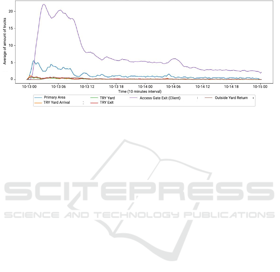
Figure 14: Average of the number of trucks per region through time for minimum queue size equals 10 for the guided pull

model.

of port operations. Additionally, an important ad-

vancement would be to develop an interactive simu-

lation with a graphical interface that allows operators

to monitor progress in real time and adjust operational

variables as needed. Expanding the guided pull con-

cept to accommodate more ships and multiple oper-

ating windows would also enhance the model’s appli-

cability in more complex scenarios.

Additionally, it would be helpful to expand the

pull operation models to include various strategies

that can address different scenarios, such as changes

in truck demand and new allocation policies. Another

important consideration is integrating additional met-

rics into the simulation. This should encompass op-

erational costs, environmental impacts (like pollutant

emissions), and maintenance expenses to analyze port

operations comprehensively.

REFERENCES

de Le

on, A. D., Lalla-Ruiz, E., Meli

an-Batista, B.,

and Moreno-Vega, J. M. (2021). A simula-

tion–optimization framework for enhancing robust-

ness in bulk berth scheduling. Engineering Applica-

tions of Artiﬁcial Intelligence, 103:104276.

Du, L., Zhang, T., and Zhang, J. (2023). Simulation of road

trafﬁc ﬂow in the port. In Nayyar, A. and Kolivand,

H., editors, Fourth International Conference on Sig-

nal Processing and Computer Science (SPCS 2023),

volume 12970, page 129700B. International Society

for Optics and Photonics, SPIE.

EMAP - Empresa Maranhense de Administrac¸

ao Portu

aria

(2024). Location of porto do itaqui. Accessed:

September 22, 2024.

Hilsdorf, W. d. C. and Nogueira Neto, M. d. S. (2015). Porto

de santos: prospecc¸

ao sobre as causas das diﬁculdades

de acesso. Gest

ao & Produc¸

ao, 23:219–231.

Iannone, R., Miranda, S., Prisco, L., Riemma, S., and

Sarno, D. (2016). Proposal for a ﬂexible discrete

event simulation model for assessing the daily oper-

ation decisions in a ro–ro terminal. Simulation Mod-

elling Practice and Theory, 61:28–46.

Menezes, G. C., Mateus, G. R., and Ravetti, M. G. (2016).

A hierarchical approach to solve a production plan-

ning and scheduling problem in bulk cargo terminal.

Computers & Industrial Engineering, 97:1–14.

Napitupulu, E., Jinca, M., and Riyanto, B. (2022). The con-

gestion factors of container truck travel from tanjung

emas port to the hinterland region. Civil Engineering

and Architecture, 10(6).

National Agency for Waterway Transportation (ANTAQ)

(2024). Database of the waterway statistical system.

Accessed: October 24, 2024.

Notteboom, T., Pallis, A., and Rodrigue, J.-P. (2022). Port

economics, management and policy. Routledge.

Simpy, T. (2020-2024). Simpy - discrete event simulation

for python. Accessed: October 23, 2024.

Uthpala, N., Hansika, N., Dissanayaka, S., Tennakoon, K.,

Dharmarathne, S., Vidanarachchi, R., Alawatugoda,

J., and Herath, D. (2023). Analyzing transportation

mode interactions using agent-based models. SN Ap-

plied Sciences, 5(12):357.

Wang, J., Zhang, X., Guo, W., Yang, Z., and Anselem

Tengecha, N. (2023). Disruption management-based

coordinated scheduling for vessels and ship loaders

in bulk ports. Advanced Engineering Informatics,

56:101989.

Optimizing Truck Flow in Ship Unloading: A Real-Time Simulation Approach for the Port of Itaqui

455