Learning Neural Velocity Fields from Dynamic 3D Scenes via
Edge-Aware Ray Sampling
Sota Ito
1
, Yoshikazu Hayashi
1
, Hiroaki Aizawa
2
and Kunihito Kato
1
1
Faculty of Engineering, Gifu University 1-1 Yanagido, Gifu City, Gifu 501-1112, Japan
2
Graduate School of Advanced Science and Engineering, Hiroshima University 1-3-2 Kagamiyama, Higashi-Hiroshima,
Hiroshima 739-0046, Japan
Keywords:
Neural Radiance Field, Physics-Informed Neural Network, Dynamic 3D Scene.
Abstract:
Neural Velocity Fields enables future frame extrapolation by learning not only the geometry and appearance
but also the velocity of dynamic 3D scenes, by incorporating physics-based constraints. While the divergence
theorem employed in NVFi enforces velocity continuity, it also inadvertently imposes continuity at the bound-
aries between dynamic objects and background regions. Consequently, the velocities of dynamic objects are
reduced by the influence of background regions with zero velocity, which diminishes the quality of extrapo-
lated frames. In our proposed method, we identify object boundaries based on geometric information extracted
from NVFi and apply the divergence theorem exclusively to non-boundary regions. This approach allows for
more accurate learning of velocities, enhancing the quality of both interpolated and extrapolated frames. Our
experiments on the Dynamic Object Dataset demonstrated a 1.6% improvement in PSNR [dB] for interpolated
frames and a 0.8% improvement for extrapolated frames.
1 INTRODUCTION
The three-dimensional world we interact with daily
operates according to physical laws, which are in-
tuitively understood by humans, allowing short-term
motion prediction. The ability to automatically model
the geometry and physical properties of dynamic 3D
scenes and predict future motion is essential in fields
such as VR/AR, gaming, and the motion picture in-
dustry.
The Neural Radiance Field (NeRF) (Mildenhall
et al., 2021) and its derivative methods (Park et al.,
2021; Pumarola et al., 2021; Cao and Johnson, 2023;
Fridovich-Keil et al., 2023; Li et al., 2021; Xian et al.,
2021) have achieved high-precision modeling of dy-
namic 3D scenes, including deformable and articu-
lated objects. These methods excel in frame interpo-
lation within the temporal range of the training data.
Nevertheless, they face limitations in frame extrapo-
lation beyond this timeframe, as they do not explicitly
learn physical properties such as velocity.
Recent studies have proposed methods that inte-
grate physics-informed constraints into NeRF-based
approaches (Chu et al., 2022; Li et al., 2024) for mod-
eling dynamic 3D scenes. These methods can simul-
taneously reconstruct the geometry, appearance, and
physical properties of complex dynamic scenes, such
as floating smoke. Neural Velocity Fields (NVFi) (Li
et al., 2024) learns the geometry, appearance, and ve-
locity of dynamic 3D scenes from multi-view videos
without the need for material properties or predefined
masks.
NVFi learns velocity by applying constraints
based on the Navier-Stokes equations, which gov-
ern fluid dynamics, and the divergence theorem. The
method captures velocity by considering temporal
continuity through the Navier-Stokes equations, while
preserving object geometry by enforcing velocity
consistency through the divergence theorem. How-
ever, since the divergence theorem imposes velocity
continuity even at the boundaries between dynamic
objects and the zero-velocity background, the veloc-
ities of dynamic objects are diminished by the influ-
ence of the zero-velocity surrounding regions, as il-
lustrated in Fig. 2. This results in reduced quality in
extrapolated frames and interpolated frames.
Our proposed method identifies object boundaries
using 3D edges computed from NVFi’s geometric in-
formation and applies the divergence theorem exclu-
sively to non-boundary regions. This approach en-
ables the learning of more accurate velocities, leading
to improved quality in both interpolated and extrapo-
Ito, S., Hayashi, Y., Aizawa, H. and Kato, K.
Learning Neural Velocity Fields from Dynamic 3D Scenes via Edge-Aware Ray Sampling.
DOI: 10.5220/0013233600003912
Paper published under CC license (CC BY-NC-ND 4.0)
In Proceedings of the 20th International Joint Conference on Computer Vision, Imaging and Computer Graphics Theory and Applications (VISIGRAPP 2025) - Volume 2: VISAPP, pages
699-706
ISBN: 978-989-758-728-3; ISSN: 2184-4321
Proceedings Copyright © 2025 by SCITEPRESS – Science and Technology Publications, Lda.
699

GT NVFi Ours
GT NVFi
Ours
GT NVFi
Ours
GT NVFi
Ours
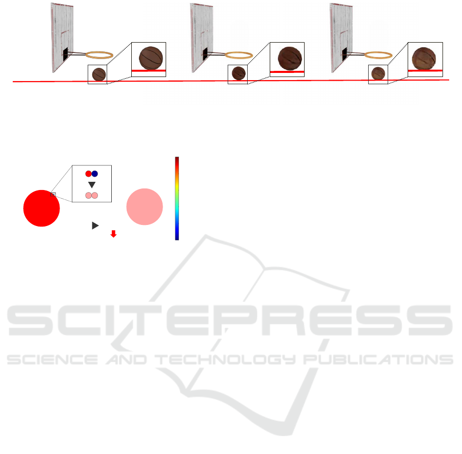
Figure 1: Comparison of rendered images for the free-falling ball sequence at timestamps beyond the training data range. Our
method effectively resolves the issue of velocity degradation observed in NVFi’s velocity learning process, enabling more
accurate velocity field estimation, leading to more accurate predictions of the ball’s terminal position.
Dynamic
Object
Velocity
High
Low
Reduction
in the velocity
ℒ
𝐝𝐢𝐯_𝐟𝐫𝐞𝐞
Dynamic Object
Velocity Reduction
Object boundary
Dynamic
Object
Figure 2: Limitation of the Divergence Theorem at Object
Boundaries. The loss function based on the divergence
theorem, expressed in Eq.(4), reduces the velocity of dy-
namic objects near object boundaries. This occurs because
the velocities of dynamic objects are influenced by the zero-
velocity background regions.
lated frames.
We evaluated our method using the Dynamic Ob-
ject Dataset (Li et al., 2024) from the original NVFi
work. The experimental results demonstrated that our
method outperformed NVFi, achieving a 1.6% im-
provement in PSNR[dB] for interpolation and a 0.8%
improvement for extrapolation.
2 RELATED WORK
2.1 Static 3D Representation
Traditional static 3D scene representation techniques
rely on discrete approaches, such as voxels (Choy
et al., 2016), point clouds (Fan et al., 2017), oc-
trees (Tatarchenko et al., 2017), and meshes (Groueix
et al., 2018). However, these representation methods
are hindered by high memory consumption and com-
putational costs in scene modeling.
Neural network-based approaches for continuous
3D scene representation have attracted significant at-
tention in recent years. These methods offer signif-
icant advantages over traditional discrete approaches
by efficiently representing continuous geometry and
appearance with low memory requirements. Notably,
Neural Radiance Field (NeRF) (Mildenhall et al.,
2021) achieved high-quality novel view synthesis by
implicitly representing rigid scenes through radiance
fields.
2.2 Dynamic 3D Representation
Since the NeRF paper was published, various NeRF-
based methods for modeling dynamic 3D scenes have
been proposed (Park et al., 2021; Pumarola et al.,
2021; Cao and Johnson, 2023; Fridovich-Keil et al.,
2023), and these methods can be classified into two
main categories.
The first approach consists of methods (Park et al.,
2021; Pumarola et al., 2021) that model temporal
variations of 3D scenes through deformations from
a canonical time frame. By representing scenes as
deformations from a canonical 3D space, these meth-
ods effectively preserve spatial consistency. However,
their accuracy degrades significantly when handling
large deformations.
The second approach includes methods (Cao and
Johnson, 2023; Fridovich-Keil et al., 2023) that
model time-varying 3D scenes by incorporating time
as an additional input alongside 3D coordinates. This
increases the input dimensionality from three to four
dimensions compared to static 3D scene representa-
tion. Consequently, these approaches require substan-
tially more memory.
These approaches are primarily designed for
frame interpolation within the temporal range of the
training data, where they demonstrate excellent per-
formance. However, they encounter significant chal-
lenges when attempting to extrapolate frames beyond
the training time range, where the model struggles to
predict motion accurately.
2.3 Physics Informed Deep Learning
Traditional deep learning methods rely on data-driven
training, learning models directly from the train-
VISAPP 2025 - 20th International Conference on Computer Vision Theory and Applications
700

ing data. However, this approach often fails to ac-
curately represent phenomena governed by physical
laws, as it does not incorporate these laws during the
learning process. Physics-Informed Neural Networks
(PINNs) (Raissi et al., 2019) enhance prediction ac-
curacy by incorporating physical laws, such as par-
tial differential equations and conservation laws, into
the loss functions. By embedding physical laws into
the model training process, PINNs can learn models
with high generalization capabilities, even with lim-
ited data or for out-of-distribution predictions. PINNs
have been successfully applied to various fields, and
methods that integrate them into dynamic 3D scene
representation (Li et al., 2024; Chu et al., 2022) have
demonstrated excellent results.
3 PRELIMINARIES: NVFi
NVFi simultaneously learns the geometry, appear-
ance, and velocity of dynamic 3D scenes from multi-
view video sequences. By explicitly modeling veloc-
ity with physics-based constraints, NVFi effectively
captures the physical dynamics of scenes. The veloc-
ity information learned through this approach enables
several challenging tasks that conventional methods
struggle with, including future frame extrapolation,
dynamic motion transfer, and semantic decomposi-
tion of 3D scenes.
3.1 Overview
The NVFi architecture comprises two networks that
are jointly optimized: (1) Keyframe Dynamic Ra-
diance Field (KDRF), which models geometry and
appearance at uniformly spaced keyframes, and (2)
Interframe Velocity Field (IVF), which predicts 3D
point velocity vectors at arbitrary time steps.
The Keyframe Dynamic Radiance Field (KDRF)
f
θ
is a network that regresses density σ and color
c = (r,g,b) from inputs of 3D coordinates p = (x,y,z),
viewing direction vector (α, β), and time t
k
, as ex-
pressed in Eq. (1). KDRF selects K keyframes from
all T frames in the training data and accepts keyframe
timestamps t
k
∈ {[T/K],2[T/K],3[T /K],·· · , T } as
input, where θ represents the learnable parameters.
(σ,c) = f
θ
(p,α,β,t
k
) = f
θ
(x,y, z,α,β,t
k
). (1)
The Interframe Velocity Field (IVF) g
φ
is a net-
work that regresses velocity vector v = (v
x
,v
y
,v
z
)
from inputs of 3D coordinates p = (x,y,z) and time t,
as expressed in Eq. (2), where φ represents the learn-
able parameters.
v = g
φ
(p,t) = g
φ
(x,y, z,t). (2)
3.2 Keyframe Dynamic Radiance Field
RGB images are rendered using KDRF f
θ
from points
sampled along the ray. For each keyframe at time
t
k
, the color
ˆ
C(r,t
k
) corresponding to ray vector r is
computed using the volume rendering technique in-
troduced in NeRF (Mildenhall et al., 2021). KDRF
f
θ
is optimized using the Photometric Loss expressed
in Eq.(3), which minimizes the diffrence between
ground truth pixel values C(r,t
k
) and their rendered
counterparts
ˆ
C(r,t
k
). Here, R denotes the set of L
ray vectors.
L
Keyframe
(R ) =
1
L
∑
r∈R
||C(r,t
k
) −
ˆ
C(r,t
k
)||
2
2
. (3)
3.3 Interframe Velocity Field
IVF g
φ
is trained using the Navier-Stokes equations
as a form of supervision, since ground truth veloc-
ity vectors are not available. To ensure consistency
in object motion during transport, IVF g
φ
must gen-
erate a divergence-free vector field that satisfies the
Navier-Stokes equations. IVF g
φ
is optimized using
the loss functions expressed in Eq.(4) and (5),which
incorporate these physical constraints. In these equa-
tions, p
n
represents points uniformly sampled across
the 3D scene, t
m
denotes time values uniformly sam-
pled from 0 to the maximum extrapolation time tmax,
and a is the acceleration term modeled by an MLP-
based network.
L
Div free
=
1
NM
N
∑
n=1
M
∑
m=1
||∇
p
n
· v(p
n
,t
m
)||, (4)
L
Momentum
=
1
NM
N
∑
n=1
M
∑
m=1




∂v(p
n
,t
m
)
∂t
m
+ (v(p
n
,t
m
) · ∇
p
n
)v(p
n
,t
m
) − a




.
(5)
When IVF g
φ
correctly transports the geometric
and appearance information represented by KDRF
f
θ
, the system can render 2D images that match
ground truth images at interframes (time steps be-
tween keyframes). Therefore, we utilize the Photo-
metric Loss computed at these interframes to optimize
IVF g
φ
.
We explain the computation algorithm: Given
S sample points {p
1
,·· · , p
s
,·· · , p
S
} along ray r
i
with viewing direction (α, β) at interframe time t
i
,
we need to determine the color and density values
{(c
1
,σ
1
),··· , (c
s
,σ
s
),··· , (c
S
,σ
S
)} for these S points
along ray r
i
. Each 3D point p
s
at time t
i
is trans-
ported to its corresponding position p
′
s at the nearest
keyframe time t
k
using IVF g
φ
, as defined in Eq.(6).
Learning Neural Velocity Fields from Dynamic 3D Scenes via Edge-Aware Ray Sampling
701







：Target 3D point
：3D point on the voxel
：Voxel size





 


Keyframe Dynamic Radiance Field


(a) Obtaining geometric information
(b) Calculation of object boundary
Edge Detection (Eq. (8))
(c) Learning Interframe Velocity Field via Edge-Aware Ray Sampling
Non-boundary weight
 

 










Velocity
MLP


 

 






Interframe Velocity Field


yt
xt
zt
yz
xy
xz
Proposed Idea
Non-boundary weight (Eq. (10))
Loss Function
Eq. (4)・Eq. (5)・Eq. (7)
Eq. (10)・Eq. (5)・Eq. (7)
Training
Eq. (10) ≒ Eq. (4) + Non-bondary weight
NVFi
Ours
Color
MLP


0.0
1.0
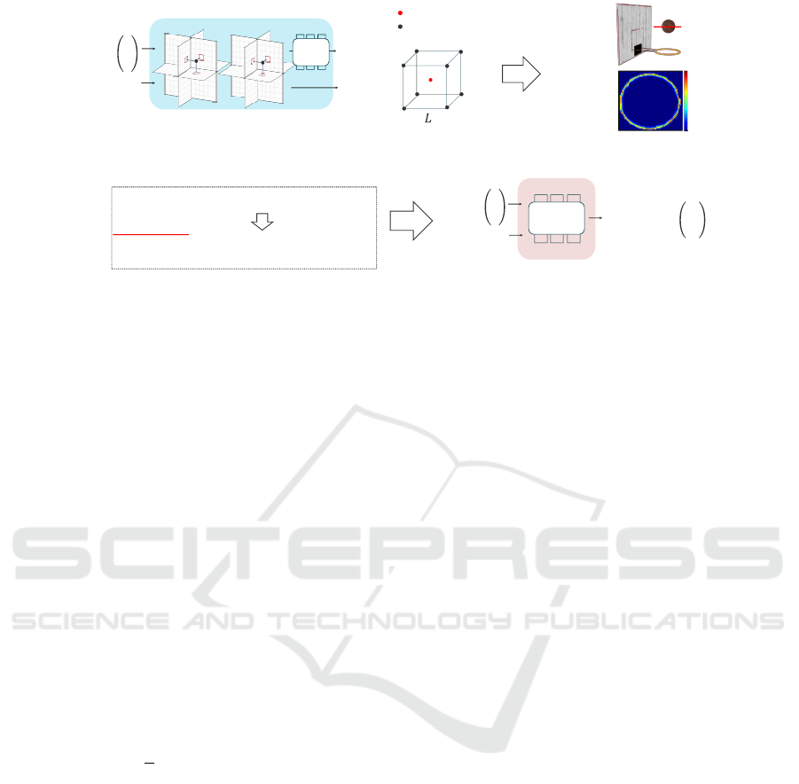
Figure 3: Overview of the proposed method. (a) Obtaining geometric information. (b) Calculation of object bound-
ary. (c) Learning Interframe Velocity Field via Edge-Aware Ray Sampling. The Keyframe Dynamic Radiance Field obtains
geometric information of 3D points on a voxel centered around the target 3D point.Based on the obtained geometric informa-
tion, we calculate object boundaries. The Interframe Velocity Field is trained with a new loss function, defined in Eq. (10),
which computes losses from the divergence theorem-based loss function (Eq. (4) exclusively in non-boundary regions.This
approach resolves the issues of the divergence theorem-based loss function (Eq. (4)) at object boundaries, as illustrated in
Fig 2.
The integration is computed using a Runge-Kutta2
solver (Chen et al., 2018).
p
′
s
= p
s
+
Z
ˆ
t
k
t
i
g
φ
(p
s
(t),t)dt. (6)
The 3D points p
s
at time t
i
and p
′
s at keyframe
time t
k
represent the same physical point transported
through IVF g
φ
. We obtain the color and density val-
ues at p
s
(time t
i
) by querying KDRF f
θ
. After ob-
taining colors and densities for all S sampling points,
we perform volume rendering to compute the color
C(r
i
,t
i
) for ray r
i
. The complete loss function is ex-
pressed in Eq.(7).
L
Interframe
(R ) =
1
L
∑
r∈R
||C(r,t
i
) −
ˆ
C(r,t
i
)||
2
2
. (7)
3.4 Problem of the Divergence Theorem
The divergence theorem-based loss function defined
in Eq.(4) serves to suppress the divergence of IVF g
φ
,
effectively enforcing continuity. This plays a crucial
role in maintaining consistency in object motion dur-
ing transport. However, this loss function enforces
velocity continuity even at the boundaries between
moving objects and static backgrounds. As shown in
Fig 2, this results in the velocities of dynamic objects
being influenced by the zero-velocity background re-
gions, leading to a reduction in their overall speed.
This prevents IVF g
φ
from learning correctly, result-
ing in reduced quality of both interpolation and ex-
trapolation. Therefore, the divergence theorem-based
loss function should not be computed at object bound-
aries where velocity changes abruptly.
4 METHOD
We propose a novel sampling method to address
the limitations of the divergence theorem-based loss
function (Eq.(4)) at object boundaries when train-
ing NVFi for dynamic 3D scene representation. The
problems described in Sec. 3.4 specifically arise at
the interfaces between dynamic objects and back-
ground regions. Our approach improves the quality
of both frame interpolation and extrapolation by en-
abling IVF g
φ
to learn more accurate velocity fields.
This is achieved through an edge-aware sampling
strategy, where edges representing object boundaries
are computed from the geometric information pro-
vided by KDRF f
θ
.
4.1 Edge Detection
Following our analysis in Sec. 3.4, we propose that
the computation of the loss term in Eq.(4) should
specifically sample 3D points from non-boundary
regions. This requires the identification of object
boundaries. For this purpose, we derive edge infor-
mation from the density values provided by KDRF
f
θ
. We define the edge measure E
n
at a 3D point p
n
using the density gradients of its neighboring points.
Specifically, we construct a voxel of size L centered
at p
n
and compute E
n
using Eq.(8), which evaluates
VISAPP 2025 - 20th International Conference on Computer Vision Theory and Applications
702

the density gradients between p
n
and its eight adja-
cent spatial points ∇r
i
.
E
n
=
q
∑
8
i=1
∇r
i
σ(p
n
,t
m
)
8
. (8)
4.2 Edge-Aware Ray Sampling
Utilizing the edge information derived in Sec. 4, we
propose a new loss function, introduced in Eq. (9),
which provides an alternative sampling strategy for
the divergence theorem-based loss in Eq.(4). In this
formulation, τ serves as the threshold parameter for
object boundary classification based on edge values,
while o
n
represents the binary boundary mask.
L
Edge mask
=
1
NM
N
∑
n=1
M
∑
m=1
||o
n
· {∇
p
n
· v(p
n
,t
m
)}||,
o
n
=
(
0 if E
n
> τ
1 otherwise
(9)
NeRF-based methods are trained to minimize
losses computed through volume rendering during
image synthesis. While density distributions along
rays remain similar under identical parameter set-
tings, the range of density values can vary depend-
ing on the initial random seed. Our approach com-
putes edge information from the density values ob-
tained from KDRF f
θ
and determines sampling re-
gions based on the boundary threshold τ. Due to vari-
ations in edge values across different seeds, the opti-
mal threshold τ for boundary classification in Eq.(9)
varies.
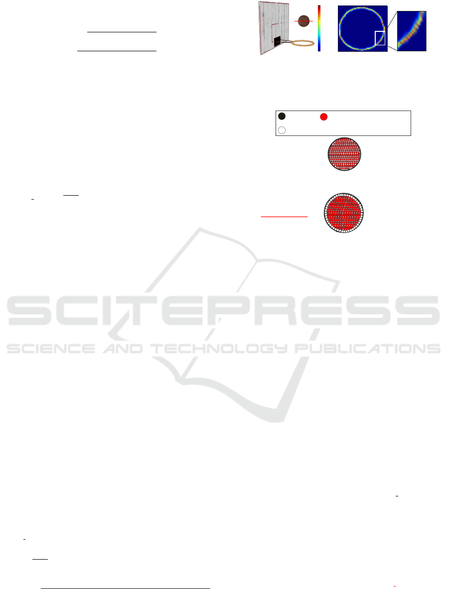
To circumvent this limitation, we introduce a
non-boundary weight w
n
derived from the com-
puted edge values, which modulates the divergence
theorem-based loss calculation near object bound-
aries. The modified training loss function is formu-
lated in Eq.(10). Given that Edge E
n
characteristi-
cally produces small values due to the influence of
voxel size L and KDRF f
θ
density values, we employ
min-max normalization on Edge E
n
. As illustrated in
Fig. 4, the resulting non-boundary weight w
n
demon-
strates notably elevated values specifically in the outer
regions of object boundaries.
L
Edge weight
=
1
NM
N
∑
n=1
M
∑
m=1
||w
n
· {∇
p
n
· v(p
n
,t
m
)}||,
w
n
= 1 −
E
n
− min(E
1
,E
2
,.. . ,E
N
)
max(E
1
,E
2
,.. . ,E
N
) − min(E
1
,E
2
,.. . ,E
N
)
.
(10)
High
Low
Figure 4: Visualization of Object Weight w
n
for Non-
boundary Regions Along the Red Line Cross-section. High
values are observed particularly at the outer regions of ob-
ject boundaries.
Calculate the Eq. (4) and Eq. (5)
for all 3D points
Calculate the Eq. (10) for 3D points
in non-edge regions
Proposed Idea
:Sampling 3D point
:Exclude 3D points from sampling
:Object
Figure 5: Sampling of Loss Functions for Training Inter-
frame Velocity Field. The proposed method computes the
divergence theorem-based loss exclusively from 3D points
in non-boundary regions.
4.3 Multi-Stage Training
The loss function in Eq.(10) requires high-fidelity
edge information obtained from KDRF f
θ
to function
effectively. Therefore, we implement a multi-stage
training strategy: in the initial training phase, we uti-
lize the original loss function from NVFi defined in
Eq.(4), then transition to our proposed loss function
expressed in Eq.(10) during the intermediate training
phase.
In the first training stage, KDRF f
θ
is optimized
using the loss functions defined in Eq.(3) and (7),
while IVF g
φ
is optimized using the loss functions
specified in Eq.(4), (5), and (7).
f
θ
←− (L
Keyframe
+ L
Interframe
),
g
φ
←− (L
Interframe
+ L
Momentum
+ L
Div free
).
(11)
In the second training stage, KDRF f
θ
is opti-
mized using the loss functions defined in Eq.(3) and
(7), while IVF g
φ
is optimized using the loss functions
specified in Eq.(4), (5), and (7).
f
θ
←− (L
Keyframe
+ L
Interframe
),
g
φ
←− (L
Interframe
+ L
Momentum
+ L
Edge weight
).
(12)
For the optimization of IVF g
φ
, we utilize the sam-
pling methodology depicted in Fig. 5 to compute the
corresponding loss functions.
Learning Neural Velocity Fields from Dynamic 3D Scenes via Edge-Aware Ray Sampling
703

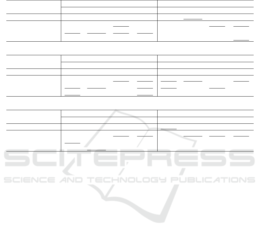
Table 1: Quantitative Comparison of Rendering Quality on the Dynamic Object Dataset. Results for interpolation during the
training period and extrapolation outside the training period.
(a) Keyframe 4.
Method
Voxel
Size
Interpolation Extrapolation
MSE↓ PSNR↑ SSIM↑ LPIPS↓ MSE↓ PSNR↑ SSIM↑ LPIPS↓
NVFi - 0.0017 29.6039 0.9708 0.0360 0.0014 28.8064 0.9768 0.0308
Ours
1.0×10
−3
0.0015 30.1055 0.9736 0.0334 0.0014 28.8018 0.9777 0.0290
1.0×10
−4
0.0016 30.1197 0.9736 0.0333 0.0014 28.8836 0.9778 0.0288
1.0×10
−5
0.0015 30.2213 0.9739 0.0330 0.0014 28.7768 0.9775 0.0290
(b) Keyframe 8.
Method
Voxel
Size
Interpolation Extrapolation
MSE↓ PSNR↑ SSIM↑ LPIPS↓ MSE↓ PSNR↑ SSIM↑ LPIPS↓
NVFi - 0.0018 29.4201 0.9700 0.0369 0.0019 28.0319 0.9742 0.0327
Ours
1.0×10
−3
0.0016 29.8007 0.9711 0.0375 0.0018 28.3921 0.9770 0.0268
1.0×10
−4
0.0017 29.7318 0.9710 0.0375 0.0018 28.3625 0.9771 0.0269
1.0×10
−5
0.0017 29.6679 0.9712 0.0375 0.0017 28.4101 0.9774 0.0267
(c) Keyframe 16.
Method
Voxel
Size
Interpolation Extrapolation
MSE↓ PSNR↑ SSIM↑ LPIPS↓ MSE↓ PSNR↑ SSIM↑ LPIPS↓
NVFi - 0.0020 28.8159 0.9685 0.0383 0.0018 27.9217 0.9739 0.0334
Ours
1.0×10
−3
0.0017 29.2815 0.9706 0.0369 0.0017 28.1306 0.9746 0.0327
1.0×10
−4
0.0019 29.1104 0.9697 0.0370 0.0017 28.0853 0.9744 0.0329
1.0×10
−5
0.0017 29.2796 0.9707 0.0365 0.0017 28.2387 0.9750 0.0324
5 EXPERIMENTS
5.1 Dataset
We evaluate our method using the Dynamic Object
Dataset introduced in (Li et al., 2024). This dataset
encompasses six distinct scenes featuring both rigid
and deformable motions in 3D space. The data collec-
tion setup comprises 15 stationary cameras, each cap-
turing 60 frames of RGB imagery. Our experimental
protocol employs the initial 45 frames from 12 cam-
eras for training, while the test set incorporates two
components: the final 15 frames from these 12 cam-
eras and the complete 60 frame sequences from the
three reserved cameras.
5.2 Evaluation Metrics
We evaluated the generation quality using three met-
rics: Peak Signal to Noise Ratio (PSNR), Structural
Similarity (SSIM) (Wang et al., 2004), and Learned
Perceptual Image Patch Similarity (LPIPS) (Zhang
et al., 2018). PSNR assesses generation quality based
on image degradation relative to ground truth images.
SSIM evaluates quality by considering three key as-
pects of human visual perception: luminance, con-
trast, and structure. LPIPS utilizes intermediate layer
outputs from pre-trained CNNs to provide a percep-
tual similarity metric that correlates with human judg-
ment. Higher values of PSNR and SSIM indicate bet-
ter generation quality, while lower LPIPS values sig-
nify superior results. We evaluate interpolation for
novel view synthesis within the training time range
(t=0.0 to t=0.75) and extrapolation for the period be-
yond training data (t=0.75 to t=1.0).
5.3 Training Details
For our implementation, we employ a HexPlane-
based model (Cao and Johnson, 2023) for KDRF f
θ
,
while IVF g
φ
is implemented using a four-layer MLP.
KDRF f
θ
is optimized using the Adam opti-
mizer (Kingma and Ba, 2014), with a ray batch size
of 1024. Our training protocol comprises two distinct
phases: the initial phase performs 30,000 iterations
with a base learning rate of 0.001. A cosine anneal-
ing scheduler with a decay factor of 0.1 is used to
adjust the learning rate. The second phase performs
another 30,000 iterations with a constant learning rate
of 0.0001.
IVF g
φ
is optimized using the Adam opti-
mizer (Kingma and Ba, 2014), with a ray batch size
VISAPP 2025 - 20th International Conference on Computer Vision Theory and Applications
704

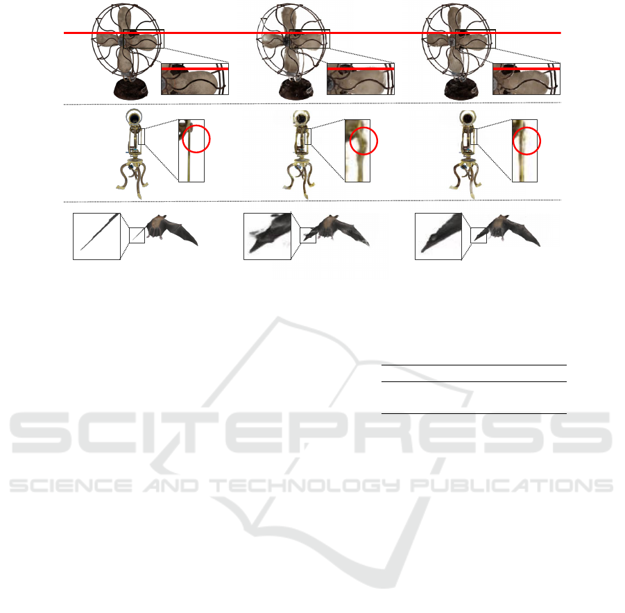
GT NVFi Ours
Figure 6: Comparison of rendered images beyond the training data range from the Dynamic Object Dataset. Our method
predicts motion in diverse scenarios, including a clockwise-rotating fan, a telescope with a rotating upper assembly, and a bat
with downward wing motion,all generated beyond the training temporal domain.
of 1024 and sample 262,144 3D points for computin
the loss terms in Eq.(4), (5), and (10). Both train-
ing phases maintain identical optimization parame-
ters: each phase executes for 30,000 iterations uti-
lizing a cosine annealing scheduler initialized with a
learning rate of 0.001 and modulated by a decay fac-
tor of 0.1.
5.4 Quantitative Evaluation
The quantitative evaluation results comparing NVFi
and our proposed method are presented in Table 1.
The results show a 1.6% improvement in frame in-
terpolation quality across all keyframe configura-
tions with our method. For frame extrapolation, our
method shows a 0.8% improvement compared to the
baseline when using 8 or 16 keyframes.
The wider temporal intervals between keyframes
explain the lack of improvement in frame extrapola-
tion quality with 4 keyframes. The computation of
non-boundary weight w
n
involves transporting den-
sity values from KDRF f
θ
at keyframe time t
k
to in-
terframe timestamps using Eq.(6). With larger inter-
vals between keyframes, the increased number of in-
tegration steps leads to a higher likelihood of accu-
mulated errors in IVF g
φ
. Consequently, when us-
ing fewer keyframes, the edge information cannot be
transported accurately, resulting in no significant im-
provement in generation quality.
Table 2: Total training time.
Method Training Time [h] ↓
NVFi 5.25
Ours 5.37
5.5 Qualitative Evaluation
Rendered images comparing NVFi and our proposed
method for extrapolated frames beyond the train-
ing data are presented in Fig 1 and 6. The results
demonstrate improved prediction of final positions in
both the free-falling ball scene and the clockwise-
rotating fan sequence, indicating successful mitiga-
tion of the velocity degradation issue in NVFi dis-
cussed in Sec. 3.4. Furthermore, enhanced object
consistency is observed in the rotating telescope and
downward-moving bat wing sequences, suggesting
that our solution to the velocity reduction problem has
led to improved consistency in object transport veloc-
ities.
5.6 Discussion
Our method demonstrates slightly superior perfor-
mance compared to NVFi. This modest improve-
ment can be explained by the limitations of the min-
max normalization used to compute the non-boundary
weight w
n
.A key limitation of this normalization pro-
cess is that when Edge E
n
values are uniformly high
across sampled 3D points, the resulting normalized
w
n
values may become inappropriately elevated, even
at genuine boundary regions. These observations
Learning Neural Velocity Fields from Dynamic 3D Scenes via Edge-Aware Ray Sampling
705

highlight the need for more sophisticated approaches
to accurately characterize non-boundary regions.
The training times for NVFi and the proposed
method using an RTX 3090 are shown in Table 2. In
the proposed method, the computation time increases
compared to NVFi because it requires calculating the
density values of neighboring regions. However, the
loss function based on the divergence theorem is ap-
plied only to 3D points with density values above a
threshold, assuming the presence of an object. Ex-
periments show that about 1% of all 3D points in the
scene exceed this threshold. As a result, the density
values of neighboring regions are calculated only for
3D points exceeding the threshold among the 262,144
sampled points. Therefore, the increase in computa-
tion time is less than initially expected.
6 CONCLUSION
This paper proposes a method to improve the quality
of synthesized frames by learning the geometry, ap-
pearance, and velocity of dynamic 3D scenes through
edge-aware sampling. We identified potential limita-
tions in accurately representing non-boundary char-
acteristics due to the min-max normalization process.
Future work will explore alternative approaches for
more accurate representation of non-boundary char-
acteristics. Furthermore, the extension of our method
to incorporate distance fields, enabling precise com-
putation of object boundary distances, presents a
promising avenue for future investigation.
REFERENCES
Cao, A. and Johnson, J. (2023). Hexplane: A fast repre-
sentation for dynamic scenes. In Proceedings of the
IEEE/CVF Conference on Computer Vision and Pat-
tern Recognition, pages 130–141.
Chen, R. T., Rubanova, Y., Bettencourt, J., and Duvenaud,
D. K. (2018). Neural ordinary differential equations.
Advances in neural information processing systems,
31.
Choy, C. B., Xu, D., Gwak, J., Chen, K., and Savarese,
S. (2016). 3d-r2n2: A unified approach for single
and multi-view 3d object reconstruction. In Computer
Vision–ECCV 2016: 14th European Conference, Am-
sterdam, The Netherlands, October 11-14, 2016, Pro-
ceedings, Part VIII 14, pages 628–644. Springer.
Chu, M., Liu, L., Zheng, Q., Franz, E., Seidel, H.-P.,
Theobalt, C., and Zayer, R. (2022). Physics informed
neural fields for smoke reconstruction with sparse
data. ACM Transactions on Graphics (ToG), 41(4):1–
14.
Fan, H., Su, H., and Guibas, L. J. (2017). A point set gener-
ation network for 3d object reconstruction from a sin-
gle image. In Proceedings of the IEEE conference on
computer vision and pattern recognition, pages 605–
613.
Fridovich-Keil, S., Meanti, G., Warburg, F. R., Recht, B.,
and Kanazawa, A. (2023). K-planes: Explicit radiance
fields in space, time, and appearance. In Proceedings
of the IEEE/CVF Conference on Computer Vision and
Pattern Recognition, pages 12479–12488.
Groueix, T., Fisher, M., Kim, V. G., Russell, B. C., and
Aubry, M. (2018). A papier-m
ˆ
ach
´
e approach to learn-
ing 3d surface generation. In Proceedings of the IEEE
conference on computer vision and pattern recogni-
tion, pages 216–224.
Kingma, D. P. and Ba, J. (2014). Adam: A
method for stochastic optimization. arXiv preprint
arXiv:1412.6980.
Li, J., Song, Z., and Yang, B. (2024). Nvfi: neural velocity
fields for 3d physics learning from dynamic videos.
Advances in Neural Information Processing Systems,
36.
Li, Z., Niklaus, S., Snavely, N., and Wang, O. (2021). Neu-
ral scene flow fields for space-time view synthesis of
dynamic scenes. In Proceedings of the IEEE/CVF
Conference on Computer Vision and Pattern Recog-
nition, pages 6498–6508.
Mildenhall, B., Srinivasan, P. P., Tancik, M., Barron, J. T.,
Ramamoorthi, R., and Ng, R. (2021). Nerf: Repre-
senting scenes as neural radiance fields for view syn-
thesis. Communications of the ACM, 65(1):99–106.
Park, K., Sinha, U., Barron, J. T., Bouaziz, S., Goldman,
D. B., Seitz, S. M., and Martin-Brualla, R. (2021).
Nerfies: Deformable neural radiance fields. In Pro-
ceedings of the IEEE/CVF International Conference
on Computer Vision, pages 5865–5874.
Pumarola, A., Corona, E., Pons-Moll, G., and Moreno-
Noguer, F. (2021). D-nerf: Neural radiance fields
for dynamic scenes. In Proceedings of the IEEE/CVF
Conference on Computer Vision and Pattern Recogni-
tion, pages 10318–10327.
Raissi, M., Perdikaris, P., and Karniadakis, G. (2019).
Physics-informed neural networks: A deep learn-
ing framework for solving forward and inverse prob-
lems involving nonlinear partial differential equations.
Journal of Computational Physics, 378:686–707.
Tatarchenko, M., Dosovitskiy, A., and Brox, T. (2017). Oc-
tree generating networks: Efficient convolutional ar-
chitectures for high-resolution 3d outputs. In Proceed-
ings of the IEEE international conference on com-
puter vision, pages 2088–2096.
Wang, Z., Bovik, A. C., Sheikh, H. R., and Simoncelli, E. P.
(2004). Image quality assessment: from error visi-
bility to structural similarity. IEEE transactions on
image processing, 13(4):600–612.
Xian, W., Huang, J.-B., Kopf, J., and Kim, C. (2021).
Space-time neural irradiance fields for free-viewpoint
video. In Proceedings of the IEEE/CVF conference on
computer vision and pattern recognition, pages 9421–
9431.
Zhang, R., Isola, P., Efros, A. A., Shechtman, E., and Wang,
O. (2018). The unreasonable effectiveness of deep
features as a perceptual metric. In Proceedings of
the IEEE conference on computer vision and pattern
recognition, pages 586–595.
VISAPP 2025 - 20th International Conference on Computer Vision Theory and Applications
706