A Hierarchical Classification for Automatic Assessment of the

Reception Quality Using Videos of Volleyball and Deep Learning

Shota Nako

, Hiroyuki Ogata

, Taiji Matsui

, Itsuki Hamada

and Jun Ohya

Department of Modern Mechanical Engineering, Waseda University, Tokyo, Japan

Department of Science and Technology, Seikei University, Tokyo, Japan

Faculty of Sport Sciences, Waseda University, Tokyo, Japan

Keywords: Volleyball, Assessment of the Reception Quality, Video Classification, Hierarchical Classification.

Abstract: To automate the assessment of the reception quality in volleyball games, this paper proposes a hierarchical

classification method that uses deep learning methods that are trained using single view videos acquired in

actual matches and the data recorded manually using Data Volley. The hierarchical classification consists of

the three steps: the first step for judging whether the player is in front of (Front) or behind (Back) the net in

the court, the second step for discriminating the best quality pass (A-pass) and second best pass (B-pass) vs.

the third best pass (C-pass), and the third step for discriminating A-pass vs B-pass. Experiments that compare

six class classification with the proposed hierarchical classification were conducted, where the former

classifies the six classes: Front A-pass, Front B-pass, Front C-pass and Back A-pass, Back B-pass, Back C-

pass. Two TimeSformer models were used as video classification models: TimeSformer-L and TimeSformer-

HR. Also, two data sets of different lengths were used. Dataset1 is longer than Dataset2. Different sampling

rates were set for each combination of dataset and model. Experimental results demonstrate that the proposed

hierarchical classification outperforms the six class classification, clarifying the best combinations of

TimeSformer model, Dataset and sampling rate.

1 INTRODUCTION

For tactical decisions and analyses of plays in

volleyball, it is useful to code and record all plays in

volleyball games. However, at present, analysts

record the code of each play manually during games,

which could pose a number of problems. That is,

analysts are required to keep concentrating on the

recording task during the game, while they sometimes

make recording errors; it takes long time to train

analysts. Obviously, these problems are not desirable.

Hence, developing a system to automate the

recording of volleyball plays is strongly demanded.

Data Volley, with which analysts record each

play, is one of the most frequetly used recording and

analysis methods currently (Silva et al., 2016). Data

Volley records four items: ‘team’, ‘player number’,

‘action’ and ‘assessment of action’. ‘Team’ indicates

which team’s player performed the action. ‘Player

number’ indicates the ID number (e.g. uniform

number) of the player who performed the action.

‘Action’ indicates the action performed by the player,

and is classified as one of the following seven actions:

service, reception (only for service), set, attack,

block, dig (reception for other than service) or free

ball (pass to the oponent court). Table 1 lists the code

of each action. ‘Assessment of the action’ indicates

whether the quality of the action was good or bad,

using a grading scale. Table 2 shows examples of

action assessments and coding.

For example, the play in which ‘Player # 4 of his

team attacked and scored’ is coded and recorded as

‘*4A#’, where * is a symbol representing that

player’s own team).

As a first step towards automating the recording

of all palys using Data Volley, this paper aims at

achieving a method for automating the assessment of

the reception quality, which is the most challenging

among the ‘assessment of the seven actions’. We

regard the assessment of the reception quality as a

video classification task. By performing hierarchical

classification utilising deep learning methods for the

single view videos acquired during actual matches

and data recorded manually using Data Volley, this

paper aims at automating the assessment equivalent

to experts’ assessment.

Nako, S., Ogata, H., Matsui, T., Hamada, I. and Ohya, J.

A Hierarchical Classiﬁcation for Automatic Assessment of the Reception Quality Using Videos of Volleyball and Deep Learning.

DOI: 10.5220/0013238000003905

Paper published under CC license (CC BY-NC-ND 4.0)

In Proceedings of the 14th International Conference on Pattern Recognition Applications and Methods (ICPRAM 2025), pages 673-680

ISBN: 978-989-758-730-6; ISSN: 2184-4313

673

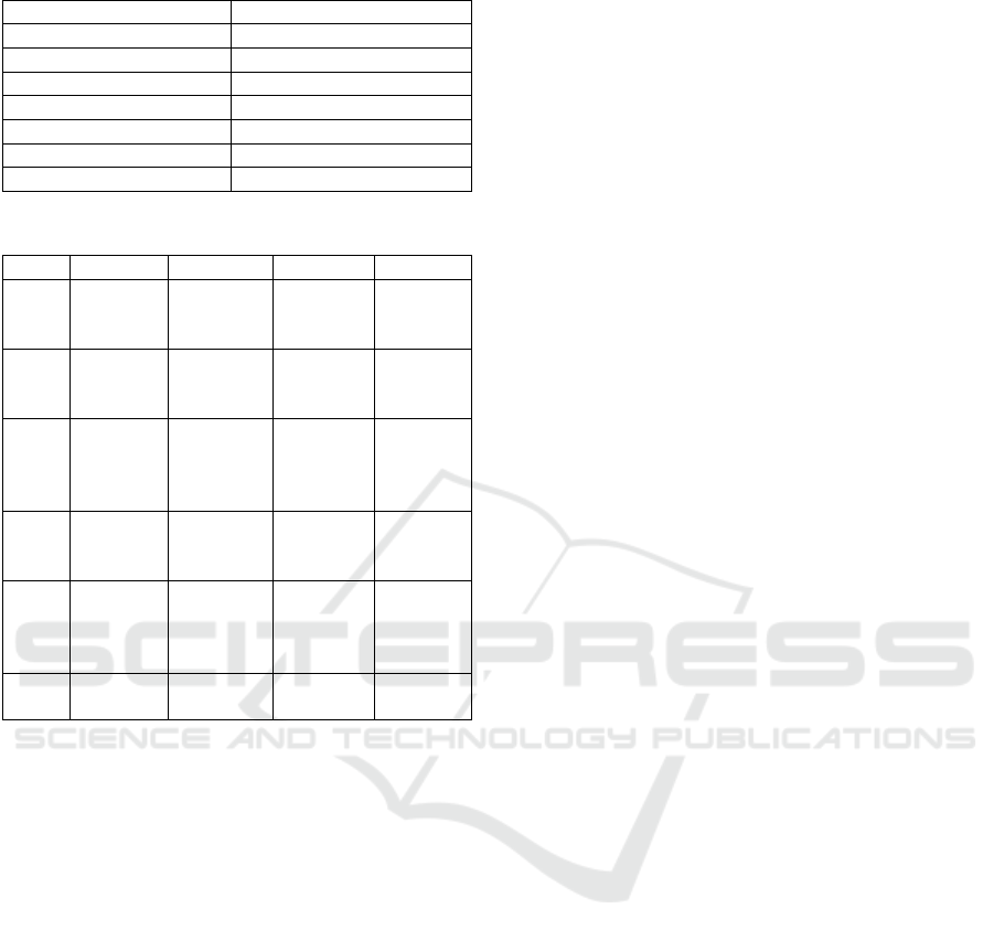
Table 1: Coding of actions.

Action Code

Serve S

Rece

tion R

Set E

Attac

Bloc

Free Ball F

Table 2: Examples of assessment of actions and coding.

Code Serve Rece

tion Attac

Bloc

= Miss

(lost

oint)

Miss (lost

point)

Miss

(lost

oint)

Miss

(lost

oint)

/ Returned

ball is D

ass

D pass Blocked Decision

(scored)

- Returned

ball is A

pass

C pass Chance

ball

One

touch

(no

effect)

! Returned

ball is B

ass

B- pass Rebound Rebound

+ Returned

ball is C

pass

B pass Rally

continues

One

touch

(with

effect)

# Ace

(

scored

)

A pass Decision

(

score

)

Decision

(

score

)

2 RELATED WORKS

2.1 Studies Related to Automating

Data Volley Recording

Several studies aim to automate Data Volley

recording, focusing on action recognition and action

assessment.

Liang et al. (2019) focused on action recognition.

They realised action recognition by utilising

handcrafted features extracted from multi-view video

acquired by four cameras and support vector

machines. However, Liang et al. did not deal with

assessing the reception quality.

Cheng, et al. (2019) proposed a method for

assessing the reception quality, similar to Liang et al.,

by extracting handcrafted features from multi-view

videos acquired by four cameras and applied machine

learning using random forest. In addition, Cheng et al.

(2022) proposed a method for assessing the reception

quality based on the position where the ball is

returned.

However, the following issues remain in the

above-mentioned Cheng et al.’s methods.

First, their criteria for evaluating each play’s

goodness are based on only the position to which the

ball is returned and the receiver's posture. This means

that their criteria are very different from experts’

assessment.

Second, difficulties in handcrafted features

include unification of assessment criteria, presence of

criteria that cannot be quantified, and unsuitability for

representing complicated actions in long-duration

videos. That is, it can be said that the handcraft

features have the limitations (Lei et al., 2019).

Third, using multi-angle cameras costs high, and

is impractical, especially for non-professional level

matches (Xia et al., 2023). In addition, due to

geometries and conditions of match venues, using

multi-angle cameras is not always possible.

2.2 TimeSformer

Video recognition based on deep learning have

attracted much attention in recent years (Bhatt et al.,

2021; Arshad, Bilal, & Gani, 2022; Guo et al., 2022).

TimeSformer (Bertasius, Wang, & Torresani,

2021) is a video classification model that exploits

Transformer (Vaswani et al., 2017), which has

achieved various SOTAs in the field of natural

language processing. For TimeSformer, Vaswani et

al. proposed an efficient architecture for

spatiotemporal attention called divided space-time

attention. This allows for more efficient processing

over much longer durations, compared to

conventional 3D CNN-based models.

In volleyball, the temporal information before and

after the play to be evaluated is important in the

assessment. Therefore, we adopt TimeSformer,

which can utilise long-duration information, as our

video classification model.

3 PROBLEM FORMULATION

This paper deals with the assessment of reception

quality as a supervised learning classification

problem.

One of this paper’s coauthors, Taiji Matsui, is the

head coach of Waseda University’s volleyball club.

In the club, the reception quality is assessed and

recorded in five levels: A pass, B pass, C pass, D pass

and miss (lost point). Of these, A pass, B pass and C

pass are receptions that led to an attack and are

assessed differently according to their quality. D pass

is a reception that goes directly back into the

ICPRAM 2025 - 14th International Conference on Pattern Recognition Applications and Methods

674

opponent’s court, and “miss” is a reception that

results in a lost point. The assessment of D pass and

miss can be considered feasible through utilising

technology such as event detection technology, and is

excluded from the classification task in this paper.

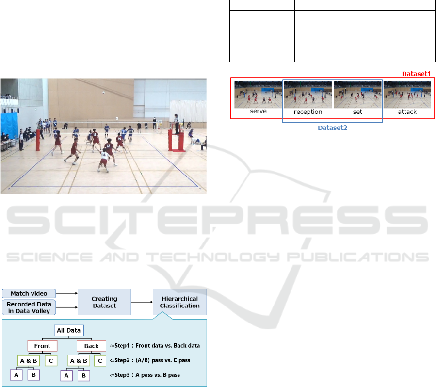
As shown in Figure 1, as only single view videos

acquired from the back of the court are used in this

paper, whether the receiver is in front of or behind the

net in the court is to be classified: i.e., the labels for

these two cases are "Front" and "Back", respectively.

Therefore, the task addressed in this paper is

formulated as a six-class classification problem:

Front-A pass, Front-B pass, Front-C pass, Back-A

pass, Back-B pass and Back-C pass.

Figure 1: Single view match video.

4 PROPOSED METHOD

The overview of the proposed method is shown in

Figure 2.

Figure 2: Overview of the proposed method.

4.1 Dataset

One data consists of a set of videos from which a

series of plays are cut out and a label for the quality

of the reception (either Front-A pass, Front-B pass,

Front-C pass, Back-A pass, Back-B pass or Back-C

pass). The video was manually cut out by the first

author of this paper. The labels were given based on

the data recorded manually using Data Volley.

In this study, two datasets with different video

lengths are created. Table 3 and Figure 3 overview the

two datasets. Dataset2 is a short version of Dataset1,

where only receptions and sets are extracted from

Dataset1.

Table 3: Overview of the datasets.

Dataset Name Description

Dataset1 Video clipping of the sequence of

play - serve, reception, set, attack

and the next action after the attack.

Dataset2 Video clipping of reception and set

only from Dataset 1.

Figure 3: Overview of the datasets.

4.2 Hierarchical Classification

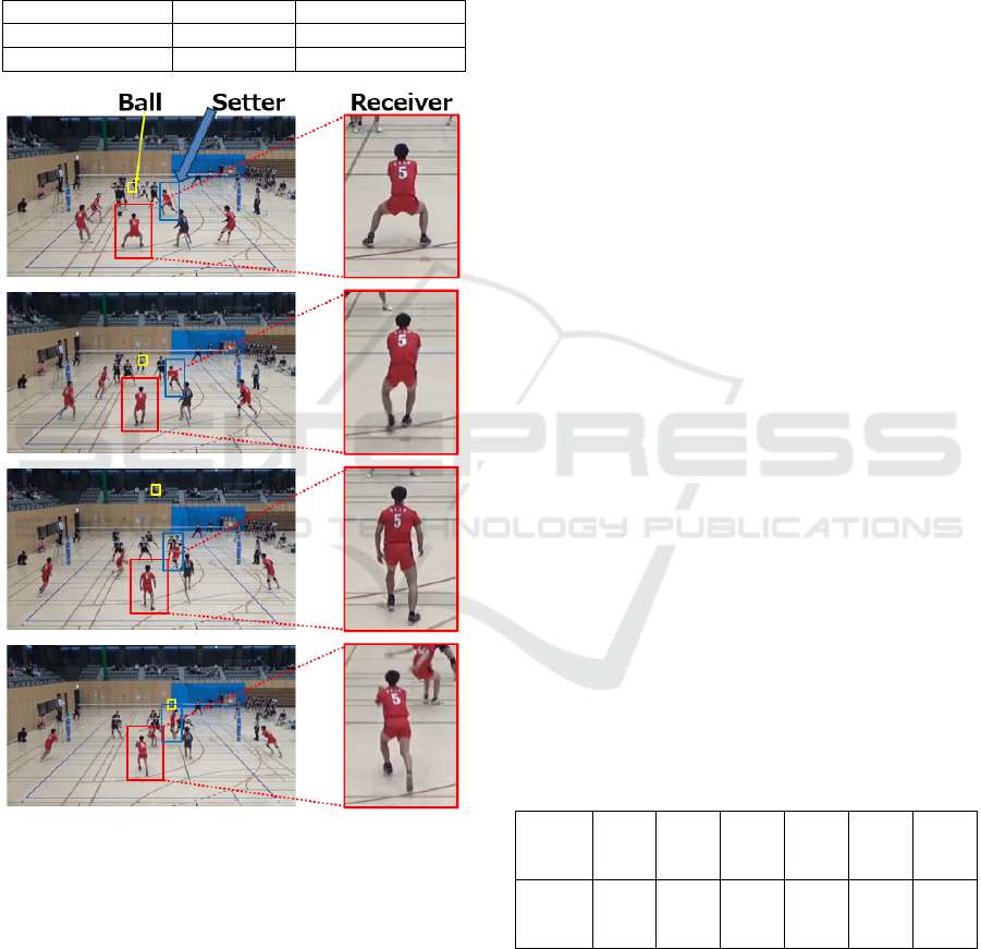
This paper focuses on the three types of reception: A

pass, B pass and C pass. Examples of A pass is shown

in Figure 4. C pass is a low-quality reception that is

difficult to connect smoothly to the attack. So, C pass

is clearly different from the A pass and B pass, which

means that C pass has different visual features. On the

other hand, both A pass and B pass can be connected

smoothly to the attack and are visually similar to each

other.

To classify visually similar A pass and B pass,

task-specific models and methods are required. For

these reasons, this paper proposes a hierarchical

approach that first classifies C pass and the other

passes, and then classifies the A pass and the B pass.

As shown in Figure 2, the proposed method

classifies receptions into six categories by the

following three steps. In Step 1, Front and Back data

with clearly different visual features are classified. In

Step 2, A pass and B pass which have similar visual

characteristics are grouped in one class ((A/B) pass),

and (A/B) pass and C pass are classified. In Step 3, A

pass and B pass, which have similar visual features,

are classified.

In each step, the TimeSformer is trained with the

respective data, creating a total of five models.

4.2.1 TimeSformer Model

As TimeSformer models, this paper uses the two

models shown in Table 4: TimeSformer-L and

TimeSformer-HR.

A Hierarchical Classiﬁcation for Automatic Assessment of the Reception Quality Using Videos of Volleyball and Deep Learning

675

TimeSformer-L allows a larger number of frames,

but as a trade-off, it requires small input image sizes.

On the other hand, TimeSformer-HR can process

larger input image sizes, but allows fewer frames to

be input. As either one of the two models could

perform better at each step of the hierarchical

classification, both models are used in this paper.

Table 4: TimeSformer model.

Model Name Ima

e Size Number of frames

TimeSforme

-L 224×224 96

TimeSforme

-HR 448×448 16

Figure 4: Examples of A pass.

4.2.2 Training Conditions

In this study, both models are fine-tuned using our

original dataset on the models pre-trained on

Kinetics-600 dataset (Carreira et al., 2018).

The dataset was stratified and randomly split into

train, validation and test sets. The split ratio was 6:2:2.

The train set was used to train the model, the

validation set was used to determine the weights to be

used during testing, and the test set was used to

calculate the accuracy of the model. The data were

split so that train, validation and test were consistent

at each step of the hierarchical classification.

It is worth noting that the dataset used in this

study was an unbalanced dataset with an uneven

number of data per class. Hence, during training,

oversampling was performed so that each class has

the same number of data as the class with the highest

number of data, where the oversampling is a process

that replicates data in classes with small numbers of

data.

The learning rate is determined by decreasing the

initial learning rate of 0.005 by a factor of 0.1 at 110

epochs and 0.01 at 140 epochs. The optimizer is SGD,

and the loss function is cross-entropy.

4.2.3 Determining the Weights to Be Used

for Testing

In this study, training was conducted in a certain

number of epochs for each step of the hierarchical

classification. In addition, an accuracy assessment

was carried out using a validation set for every five

epochs; the weights at the epoch that achieved the

highest accuracy in the validation set were used for

testing.

5 EXPERIMENTAL RESULTS

5.1 Dataset

The dataset was created based on 11 match videos

provided by Waseda University’s volleyball club

mentioned in Section 3 and the data recorded using

Data Volley. The resolution of each frame of the

videos is 1280×720, and the frame rate of the videos

is 29.97 fps. The number of data per class is shown in

Table 5.

Table 5: Number of data.

Class

Name

Fron

t-A

ass

Fron

t-B

ass

Fron

t-C

ass

Back

-A

ass

Back

-B

ass

Back

-C

ass

Num

Data

142 494 152 125 476 119

5.2 Determining Hyperparameters

Initially, candidate sampling rate values that improve

the accuracy of the model were searched, where the

sampling rate is a parameter that defines the interval

ICPRAM 2025 - 14th International Conference on Pattern Recognition Applications and Methods

676

between each successive frames extracted when a

video is input to the model.

The sampling rate values selected for each

combination of the datasets and TimeSformer models

are shown in Table 6. In the subsequent experiments,

training, validation and testing were carried out under

the conditions listed in Table 6.

Table 6: Combination of dataset, TimeSformer model and

sampling rate.

Dataset TimeSformer Model Sampling Rate

Dataset1 L 2

Dataset2 L 1

Dataset2 HR 6

5.3 6- Class Classification

To compare with the hierarchical classification, a

model that classifies the six classes was trained.

Using the trained model, tests for classifying the six

classes were carried out. The results are shown in

Table 7. Figure 5, whose vertical and horizontal axes

indicate the true and predicted labels, respectively,

shows the confusion matrix under the condition in

which the best accuracy was obtained, where the

maximum number of epochs is 150.

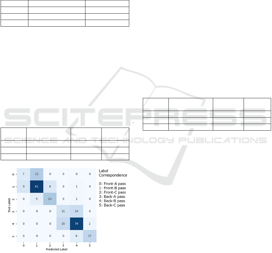
Table 7: 6 Class classification results.

Dataset TimeSformer

Model

Sampling

Rate

Accuracy

Dataset1 L 2 0.6987

Dataset2 L 1 0.7252

Dataset2 HR 6 0.7185

Figure 5: 6-Class classification confusion matrix.

Table 7 shows that the combination of Dataset2,

model L and a sampling rate of 1 achieved the highest

accuracy of 0.7252.

Figure 5 also shows that out of the 158 Front data,

there were 2 cases (1.27%) in which Front data were

misclassified as Back data. Furthermore, out of the

156 true positive data for the Front data, the number

of misclassifying Front-(A/B) pass as Front-C pass

and vice versa were 13 (8.33%). Out of the 144 true

positive data for the Back data, the number of

misclassifying Back-(A/B) pass as Back-C pass and

vice versa were 8 (5.56%). Out of the 119 true

positive data for the Front-(A/B) pass, the number of

misclassifying the Front-A pass as the Front-B pass

and vice versa was 31 (26.05%). Out of the 119 true

positive data for the Back-(A/B) pass, the number of

misclassifying the Back-A pass as the Back-B pass

and vice versa was 29 (24.37%).

5.4 Hierarchical Classification

5.4.1 Step1: Front Data vs. Back Data

Table 8 shows the results of Step 1 of the hierarchical

classification: i.e. the results of classifying Front data

and Back data, where the maximum number of

epochs is 15.

Table 8: Results of Step 1 of Hierarchical classification.

Dataset TimeSformer

Model

Sampling

Rate

Accuracy

Dataset1 L 2 0.9967

Dataset2 L 1 1.0000

Dataset2 HR 6 1.0000

According to Table 8, the combination of Dataset2,

model L and sampling rate = 1 and combination of

Dataset2 model HR and sampling rate = 6 give the

highest accuracy of 1.0000.

5.4.2 Step2: (A/B) Pass vs. C Pass

Table 9 shows the results of Step 2 of the hierarchical

classification: i.e. the results of classifying the (A/B)

pass and C-pass. Figures 6 and 7 show the confusion

matrices under the most accurate conditions for the

Front and Back data, respectively, where the

maximum number of epochs is 50.

Table 9 shows that the combination of Dataset2,

model HR and sampling rate = 6 achieved the highest

accuracy for both Front and Back data, with the

accuracies of 0.9494 and 0.9306, respectively.

Furthermore, Figure 6 shows that out of the 158 Front

data, the number of misclassifying the Front-(A/B)

pass as the Front-C pass and vice versa was 8

(5.063%). Figures 7 shows that out of the 144 Back

data, the number of misclassifying the Back-(A/B)

pass as the Back-C pass and vice versa was 10

(6.944%).

A Hierarchical Classiﬁcation for Automatic Assessment of the Reception Quality Using Videos of Volleyball and Deep Learning

677

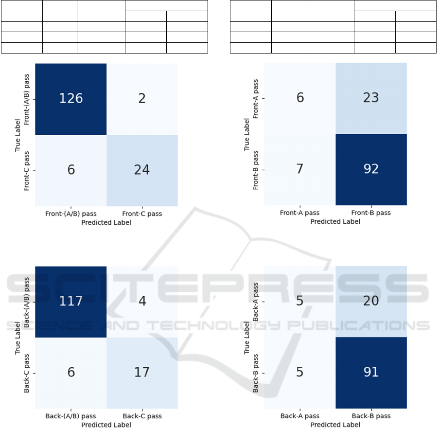
Table 9: Results of Step 2 of Hierarchical classification.

Dataset Model Sampling

Rate

Accurac

Front Bac

Dataset1 L 2 0.8481 0.9236

Dataset2 L 1 0.9114 0.9167

Dataset2 HR 6 0.9494 0.9306

Figure 6: Hierarchical classification step2 (Front data)

confusion matrix.

Figure 7: Hierarchical classification step2 (Back data)

confusion matrix.

5.4.3 Step3: A Pass vs. B Pass

Table 10 shows the results of Step 3 of the

hierarchical classification: i.e. the results of

classifying the A-pass and B-pass. Figures 8 and 9

show the confusion matrices under the most accurate

conditions for the A-pass and B-pass, respectively,

where the maximum number of epochs is 150.

Table 10: Results of Step 3 of Hierarchical classification.

Dataset Model Sampling

Rate

Accurac

Front Bac

Dataset1 L 2 0.7422 0.7107

Dataset2 L 1 0.7656 0.7934

Dataset2 HR 6 0.6640 0.7603

Figure 8: Hierarchical classification step3 (Front data)

confusion matrix.

Figure 9: Hierarchical classification step3 (Back data)

confusion matrix.

Table 10 shows that the combination of Dataset2,

model L and a sampling rate = 1 achieved the highest

accuracy for both Front and Back data, with the

accuracies of 0.7656 and 0.7934, respectively.

Furthermore, Figures 8 shows that out of the 128

Front-(A/B) pass, the number of misclassifying the

Front-A pass as the Front-B pass and vice versa was

30 (23.44%). Figure 9 shows that out of the 121 Back-

(A/B) pass, the number of misclassifying the Back-A

pass as the Back-B pass and vice versa was 25

ICPRAM 2025 - 14th International Conference on Pattern Recognition Applications and Methods

678

(20.66%). In particular, there are many cases in which

A pass is misclassified as B pass.

6 DISCUSSION

6.1 Comparison of 6- Class

Classification and Hierarchical

Classification

Figure 5 shows that there were 2 misclassifications of

Front data as Back data in the 6-class classification.

In contrast, Table 8 shows that the accuracy of step 1

of the hierarchical classification was 1.0000 and did

not result in misclassification. Figures 5 to 9 also

show that the number of misclassifications and error

rates were lower in hierarchical classification for A

pass, B pass and C pass classification in all cases

except for the Back data in step 2. Hence, it can be

said that the hierarchical classification outperforms

the 6-class classification in terms of reducing the risk

of misclassification. Meanwhile, it should be noted

that hierarchical classification has a cascading nature,

which may propagate errors from previous steps.

Another advantage of the hierarchical

classification compared to the 6-class classification is

that it allows different approaches to the tasks and

characteristics of each step. In other words, the

introduction of the hierarchical classification has

succeeded in subdividing the problem of automatic

assessment of the reception quality. Therefore, in the

future, it is expected to achieve methods that are more

suitable for the tasks and characteristics of each step.

6.2 Discussion at Each Step of the

Hierarchical Classification

Tables 9 and 10 show that the higher accuracy was

achieved using Dataset2 for both step2 and step3 than

Dataset1. Whereas Dataset1 is long videos that cut

out the sequence of serve, reception, set, attack and

the next action after the attack, Dataset2 is short

videos that cut out only the reception and set from

Dataset1. Therefore, the results suggest that it is more

effective for the classification to focus on the play

before and after the reception, rather than the entire

series of plays, for assessing the reception quality. In

particular, the setter’s movement is an important

element in the assessment of the reception quality,

and the fact that the setter’s movements appear in

many frames in the entire video in Dataset2 might

contribute to improving the accuracy.

Table 9 also shows that the combination of

Dataset2, model HR and a Sampling rate = 6 achieved

the highest accuracy for both Front and Back data in

the classification of (A/B) pass and C pass.

TimeSformer-L is a model that allows for longer

video input, whereas TimeSformer-HR is a model

that allows for larger image sizes. This suggests that

spatial information is more important than temporal

information in classifying (A/B) pass and C pass. In

addition, compared to (A/B) pass, the C pass video is

characterised by a larger movement of the setter,

which is important for the assessment of the reception

quality. Hence, it is possible that the TimeSformer-

HR, which can input larger image sizes, may have

adequately captured spatially significant changes,

leading to the improved accuracies.

On the other hand, Table 10 shows that the

combination of Dataset2, model L and sampling rate

= 1 achieved the highest accuracy for both Front and

Back data in the classification of A pass and B pass.

This suggests that, conversely, in the classification of

A pass and B pass temporal information is more

important than spatial information.

In addition, the highest accuracy in classifying A

pass and B pass was 0.7656 and 0.7934 for the Front

and Back data, respectively, which is lower than the

classification accuracy of (A/B) pass and C pass. This

could be due to the visual similarity of the A pass and

B pass. In this paper, the entire video was simply used

as the input for learning, but in the future, further

accuracy improvements can be expected by

effectively utilising local information such as setter’s

movements.

7 CONCLUSIONS AND FUTURE

WORK

This paper has explored methods for recording each

play in volleyball games using Data Volley,

particularly focusing on automating the assessment of

the reception quality, which is still a major issue in

the ‘assessment of actions’. This paper treats the

assessment of the reception quality as a video

classification task, and has proposed a hierarchical

classification method that uses deep learning methods

that are trained using single view videos acquired in

actual matches and the data recorded manually using

Data Volley. The hierarchical classification consists

of the three steps: the first step for the Front vs Back,

the second step for the (A/B)-pass vs C-pass, and the

third step for the A-pass vs B-pass.

A Hierarchical Classiﬁcation for Automatic Assessment of the Reception Quality Using Videos of Volleyball and Deep Learning

679

Experiments that compare six class classification

with the proposed hierarchical classification were

conducted, where the former classifies the six classes:

Front A-pass, Front B-pass, Front C-pass and Back

A-pass, Back B-pass, Back C-pass. Two

TimeSformer models were used as video

classification models: TimeSformer-L and

TimeSformer-HR. Also, two data sets of different

lengths were used, where Dataset1 is long videos that

cut out the sequence of serve, reception, set, attack

and the next action after the attack, and Dataset2 is

short videos that cut out only the reception and set

from Dataset1. To improve accuracy, the optimum

sampling rate was set for each combination of dataset

and model, and training, validation and testing were

carried out under these conditions.

The best accuracy by the six class classification is

only 72.5%.

In contrast, in the hierarchical classification, the

Step 1, which classifies Front and Back data,

achieved 100% accuracy. The Step 2, which classifies

(A/B)-pass and C-pass, achieved 94.94% and 93.06%

accuracies on Front and Back data, respectively,

under the combination of Dataset2, model HR and

sampling rate = 6. The Step 3, which classifies A-pass

and B-pass, achieved 76.56% and 79.34% accuracies

on Front and Back data, respectively, under the

combination of Dataset2, model L and sampling rate

= 1.

The hierarchical classification did not result in

misclassification of Front and Back data. It also

reduced the number of misclassifications and the

error rate in all the cases except for one case for step2.

Thus, it can be said that the hierarchical classification

is superior to the six class classification in terms of

reducing the risk of misclassification. Another

advantage over the six class classification is that

hierarchical one allows a separate approach to the

tasks and characteristics of each step, successfully

subdividing the problem of automating the

assessment of the reception quality.

In the future, we will focus on developing a

method for classifying A- and B-passes, where the

current accuracies are relatively low. In particular, we

aim to improve the accuracy through a method that

effectively use local information, such as the setter’s

movement, which is considered important in the

assessment of the reception quality.

Furthermore, hierarchical classification is

expected to be applied to other sports videos.

REFERENCES

Silva, M., Marcelino, R., Lacerda, D., & João, P.V. (2016).

Match analysis in Volleyball: A systematic review.

Montenegrin Journal of Sports Science and Medicine,

5(1), 35-46.

Liang, L., Cheng, X., & Ikenaga, T. (2019). Team

formation mapping and sequential ball motion state

based event recognition for automatic data volley.

Proceedings of the 16th International Conference on

Machine Vision Applications, MVA 2019, 8757998.

doi: 10.23919/MVA.2019.8757998

Cheng, X., Liu, Y., & Ikenaga, T. (2019). 3D global and

multi-view local features combination based qualitative

action recognition for volleyball game analysis. IEICE

Transactions on Fundamentals of Electronics,

Communications and Computer Sciences, E102A(12),

1891-1899. doi: 10.1587/transfun.E102.A.1891

Cheng, X., Liang, L., & Ikenaga, T. (2022). Automatic data

volley: game data acquisition with temporal-spatial

filters. Complex and Intelligent Systems, 8(6), 4993-

5010. doi: 10.1007/s40747-022-00752-3

Lei, Q., Du, J.X., Zhang, H.B., Ye, S., & Chen, D.S. (2019).

A survey of vision-based human action evaluation

methods. Sensors (Switzerland), 19(19), 4129. doi:

10.3390/s19194129

Xia, H., Tracy, R., Zhao, Y., Wang, Y., Wang, Y.F., & Shen,

W. (2023). Advanced Volleyball Stats for All Levels:

Automatic Setting Tactic Detection and Classification

with a Single Camera. IEEE International Conference

on Data Mining Workshops, ICDMW, 1407-1416. doi:

10.1109/ICDMW60847.2023.00179

Bhatt, D., Patel, C., Talsania, H., Patel, J., Vaghela, R.,

Pandya, S., … Ghayvat, H. (2021). Cnn variants for

computer vision: History, architecture, application,

challenges and future scope. Electronics (Switzerland),

10(20), 2470. doi: 10.3390/electronics10202470

Arshad, M.H., Bilal, M., & Gani, A. (2022). Human

Activity Recognition: Review, Taxonomy and Open

Challenges. Sensors, 22(17), 6463. doi:10.3390/s2217

6463

Guo, M.H., Xu, T.X., Liu, J.J., Liu, Z.N., Jiang, P.T., Mu,

T.J., ... Hu, S.M. (2022). Attention mechanisms in

computer vision: A survey. Computational Visual

Media, 8(3), 331-368. doi: 10.1007/s41095-022-0271-

Bertasius, G., Wang, H., & Torresani L. (2021). Is Space-

Time Attention All You Need for Video

Understanding? Proceedings of Machine Learning

Research, 139, 813-824. https://arxiv.org/pdf/2102.05

095

Vaswani, A., Shazeer, N., Parmar, N., Uszkoreit, J., Jones,

L., Gomez, A.N., ... Polosukhin, I. (2017). Attention is

all you need. Advances in Neural Information

Processing Systems, 2017-December, 5999-6009.

https://arxiv.org/pdf/1706.03762

Carreira, J., Noland, E., Banki-Horvath, A., Hillier, C., &

Zisserman, A. (2018). A short note about kinetics-

600.

arXiv preprint arXiv:1808.01340.

ICPRAM 2025 - 14th International Conference on Pattern Recognition Applications and Methods

680