Proposing Hierarchical Goal-Conditioned Policy Planning in Multi-Goal
Reinforcement Learning
Gavin B. Rens
a
Computer Science Division, Stellenbosch University, Stellenbosch, South Africa
Keywords:
Reinforcement Learning, Monte Carlo Tree Search, Hierarchical, Goal-Conditioned, Multi-Goal.
Abstract:
Humanoid robots must master numerous tasks with sparse rewards, posing a challenge for reinforcement
learning (RL). We propose a method combining RL and automated planning to address this. Our approach
uses short goal-conditioned policies (GCPs) organized hierarchically, with Monte Carlo Tree Search (MCTS)
planning using high-level actions (HLAs). Instead of primitive actions, the planning process generates HLAs.
A single plan-tree, maintained during the agent’s lifetime, holds knowledge about goal achievement. This hi-
erarchy enhances sample efficiency and speeds up reasoning by reusing HLAs and anticipating future actions.
Our Hierarchical Goal-Conditioned Policy Planning (HGCPP) framework uniquely integrates GCPs, MCTS,
and hierarchical RL, potentially improving exploration and planning in complex tasks.
1 INTRODUCTION
Humanoid robots have to learn to perform several, if
not hundreds of tasks. For instance, a single robot
working in a house will be expected to pack and un-
pack the dishwasher, pack and unpack the washing
machine, make tea and coffee, fetch items on demand,
tidy up a room, etc. For a reinforcement learning (RL)
agent to discover good policies or action sequences
when the tasks produce relatively sparse rewards is
challenging (Pertsch et al., 2020; Ecoffet et al., 2021;
Shin and Kim, 2023; Hu et al., 2023; Li et al., 2023).
Except for (Ecoffet et al., 2021), the other four ref-
erences use hierarchical approaches. This paper pro-
poses an approach for agents to learn multiple tasks
(goals) drawing from techniques in hierarchical RL
and automated planning.
A high-level description of our approach fol-
lows. The agent learns short goal-conditioned poli-
cies which are organized into a hierarchical structure.
Monte Carlo Tree Search (MCTS) is then used to plan
to complete all the tasks. Typical actions in MCTS are
replaced by high-level actions (HLAs) from the hier-
archical structure. The lowest-level kind of HLA is
a goal-conditioned policy (GCP). Higher-level HLAs
are composed of lower-level HLAs. Actions in our
version of MCTS can be any HLAs at any level. We
assume that the primitive actions making up GCPs are
given/known. But the planning process does not op-
a
https://orcid.org/0000-0003-2950-9962
4, 13
5, 16 10, 5
2, 11
1, 12
10, 9
4, 11
4, 9
4, 15
1
4
3
5
2
6
9
14
4, 7
6, 5
15
18
2, 1
2, 5
21
9, 2
5, 2
23
24
7, 10
7
10
8
6, 13
11
7, 16
11, 16
12
16, 13
15, 16
13
16
17
12, 3
13, 6
22
8, 3
20
19
HLA1
HLA3
HLA4
HLA5
HLA2
HLA6
HLA7
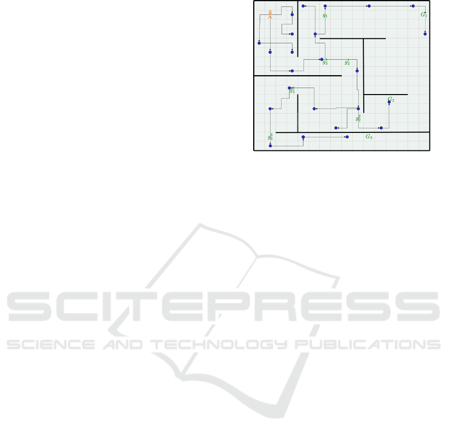
Figure 1: Complete plan-tree corresponding to the maze
grid-world. Note that HLA7 is composed of HLA1, HLA3
and HLA6, in that order.
erate directly on primitive actions; it involves gener-
ating HLAs during planning.
A single plan-tree is grown and maintained dur-
ing the lifetime of the agent. The tree constitutes
the agent’s knowledge about how to achieve its goals
(how to complete its tasks). Figure 1 is a complete
plan-tree for the environment depicted in Figure 2.
Rens, G. B.
Proposing Hierarchical Goal-Conditioned Policy Planning in Multi-Goal Reinforcement Learning.
DOI: 10.5220/0013238900003890
Paper published under CC license (CC BY-NC-ND 4.0)
In Proceedings of the 17th International Conference on Agents and Artificial Intelligence (ICAART 2025) - Volume 1, pages 507-514
ISBN: 978-989-758-737-5; ISSN: 2184-433X
Proceedings Copyright © 2025 by SCITEPRESS – Science and Technology Publications, Lda.
507

The idea is to associate a value for each goal with
every HLA (at every level) discovered by the agent
so far. An agent becomes more sample efficient by
reusing some of the same HLAs for reaching different
goals. Moreover, the agent can reason (search) faster
by looking farther into the future to find more valu-
able sequences of actions than if it considered only
primitive actions. This is the conventional reason for
employing hierarchical planning; see the papers ref-
erenced in Section 2.2 and Section 3
For ease of reference, we call our new approach
HGCPP (Hierarchical Goal-Conditioned Policy Plan-
ning). To the best of our knowledge, at the time
of writing, no-one has explicitly combined goal-
conditioned policies, MCTS, and hierarchical RL in a
single framework. This combination could potentially
lead to more efficient exploration and planning in
complex domains with multiple long-horizon goals.
The rest of the paper is organized as follows. Sec-
tion 2 provides the necessary background theory. Sec-
tion 3 reviews the related work. Section 4 presents our
framework (or family of algorithms). We also pro-
pose some novel and existing techniques that could
be used for implementing an instance of HGCPP. In
Section 5 we further analyze our proposed approach
and make further suggestions to improve it. As this is
early-stage research, there is no evaluation yet.
2 BACKGROUND
2.1 Goal-Conditioned Reinforcement
Learning
Reinforcement learning (RL) is based on the Markov
decision process (MDP). An MDP is described as a
tuple ⟨S,A,T, R,γ⟩, where S is a set of states, A is a
set of (primitive) actions, T is a transition function
(the probability of reaching a state from a state via
an action), R : S × A × S 7→ R and γ is the discount
factor. The value of a state s is the expected total
discounted reward an agent will get from s onward,
that is, V (s)
.
= E
s
t+1
∼T (s
t
,a
t
,·)
[
∑
∞
t=0
γ
t
R(s
t
,a
t
,s
t+1
) |
s
0
= s], where s
t+1
is the state reached by execut-
ing action a in state s
t
. Similarly, the value of ex-
ecuting a in s is defined by Q(a, s)
.
= R(s,a, s
′
) +
γ
∑
s
′
∈S
T (s,a,s
′
)V (s
′
). We call it the Q function and
its value is a q-value. The aim in MDPs and RL is
to maximize V(s) for all reachable states s. A policy
π : S 7→ A tells the agent what to do: execute a = π(s)
when in s. A policy can be defined in terms of a Q
function: ∀s ∈ S,π(s)
.
= argmax
a∈A
Q(a,s). It is thus
desirable to find ‘good’ q-values (see later).
Goal-conditioned reinforcement learning (GCRL)
(Schaul et al., 2015; Liu et al., 2022) is based on the
GCMDP, defined as the tuple ⟨S,A,T,R,G, γ,⟩, where
S, A, T and γ are as before, G is a set of (desired)
goals and R : S × A × S × G 7→ R is goal-conditioned
reward function. In GCRL, the value of a state and the
Q function are conditioned on a goal g ∈ G: V (s,g),
respectively, Q(a,s,g). A goal-conditioned policy: π :
S × G 7→ A; π(s,g) is the action to execute in state s
towards achieving g.
2.2 Hierarchical Reinforcement
Learning
Traditionally, hierarchical RL (HRL) has been a
divide-and-conquer approach, that is, determine the
end-goal, divide it into a set of subgoals, then select
or learn the best way to reach the subgoals, and fi-
nally, achieve each subgoal in an order appropriate to
reach the end-goal.
“Hierarchical Reinforcement Learning (HRL)
rests on finding good re-usable temporally extended
actions that may also provide opportunities for state
abstraction. Methods for reinforcement learning can
be extended to work with abstract states and actions
over a hierarchy of subtasks that decompose the orig-
inal problem, potentially reducing its computational
complexity.” (Hengst, 2012)
“The hierarchical approach has three challenges
[619, 435]: find subgoals, find a meta-policy over
these subgoals, and find subpolicies for these sub-
goals.” (Plaat, 2023)
The divide-and-conquer approach can be thought
of as a top-down approach. The approach that
our framework takes is bottom-up: the agent learns
‘skills’ that could be employed for achieving different
end-goals, then memorizes sets of connected skills as
more complex skills. Even more complex skills may
be memorized based on less complex skills, and so
on. Higher-level skills are always based on already-
learned skills. In this work, we call a skill (of any
complexity) a high-level action.
2.3 Monte Carlo Tree Search
The version Monte Carlo tree search (MCTS) we are
interested in is applicable to single agents based on
MDPs (Kocsis and Szepesvari, 2006).
An MCTS-based agent in state s that wants to se-
lect its next action loops thru four phases to generate
a search tree rooted at a node representing s. Once
the agent’s planning budget is depleted, it selects the
action extending from the root that was most visited
(see below) or has the highest q-value. While there
ICAART 2025 - 17th International Conference on Agents and Artificial Intelligence
508

still is planning budget, the algorithm loops thru the
following phases (Browne et al., 2012).
Selection. A route from the root until a leaf node
is chosen. (For discrete problems, a node is a leaf
if not all actions have been tried at least once in
that node.) Let UCBX : Nodes × A 7→ R denote any
variant of the Upper Confidence Bound, like UCB1
(Kocsis and Szepesvari, 2006). For every non-leaf
node n in the tree, follow the path via action a
∗
=
argmax
a∈A
UCBX(n,a).
Expansion. When a leaf node n is encountered, select
an action a not yet tried in n and generate a new node
representing s
′
as child of n.
Rollout. To estimate a value for s
′
(or n
′
represent-
ing it), simulate one or more Monte Carlo trajecto-
ries (rollouts) and use them to calculate a reward-to-
go from n
′
. If the rollout value for s
′
is V (s
′
), the
Q(a,s) can be calculated.
Backpropagation. If n
′
has just been created and
the q-value associated with the action leading to it
has been determined, then all action branches on the
path from the root till n must be updated. That is, the
change in value at the end of a path must be propa-
gated bach up the tree.
In this paper, when we write f (n) (where n might
have indices and f is some function), we generally
mean f (n.s) and f (s
′
), where n.s = s
′
is the state rep-
resented by node n.
3 RELATED WORK
The areas of hierarchical reinforcement learning
(HRL) and goal-conditioned reinforcement learning
(GCRL) are very large. The overlapping area of goal-
conditioned hierarchical RL is also quite large. Ta-
ble 1 shows where some of the related work falls
with respect to the dimensions of 1) goal-conditioned
(GC), 2) hierarchical (H), 3) planning (P) and 4) RL.
See the list below for the reference corresponding to
the numbers shown in the table.
1 (Kulkarni et al., 2016)
2 (Andrychowicz et al., 2017)
3 (Pinto and Coutinho, 2019)
4 (Pertsch et al., 2020)
5 (Lu et al., 2020)
6 (Ecoffet et al., 2021)
7 (Fang et al., 2022)
8 (Li et al., 2022)
9 (Mezghani et al., 2022)
10 (Yang et al., 2022)
11 (Castanet et al., 2023)
12 (Shin and Kim, 2023)
13 (Zadem et al., 2023)
14 (Hu et al., 2023)
15 (Li et al., 2023)
16 (Castanet et al., 2023)
17 (Wang et al., 2024)
We do not have the space for a full literature
survey of work involving all combinations of two
or more of these four dimensions. Nonetheless, we
Table 1: Related work categorized over four dimensions.
The numbers map to the literature in the list below.
only RL RL+P only P
only GC 6, 16, 2 9
GC+H 11, 12, 13,
14
1, 3, 7, 8,
10, 17,
HGCPP
4, 15
only H 5
believe that the work mentioned in this section is
fairly representative of the state of the art relating to
HGCPP.
We found only two papers involving hierarchical
MCTS: (Lu et al., 2020) does not involve RL nor
goal-conditioning, nor multiple goals. It is placed
in the bottom right corner of Table 1. The work of
Pinto and Coutinho (2019) is closest to our frame-
work. They propose a method for HRL in fighting
games using options with MCTS. Instead of using
all possible game actions, they create subsets of ac-
tions (options) for specific gameplay behaviors. Each
option limits MCTS to search only relevant actions,
making the search more efficient and precise. Op-
tions can be activated from any state and terminate
after one step, allowing the agent to learn when to use
and switch between different options. The approach
uses Q-learning with linear regression to approximate
option values, and an ε-greedy policy for option se-
lection. They call their approach hierarchical simply
because it uses options. HGCPP has hierarchies of ar-
bitrary depth, whereas theirs is flat. They do not gen-
erate subgoals, while HGCPP generates reachable and
novel behavioral goals to promote exploration. One
could view their approach as being implicitly multi-
goal. Pinto and Coutinho (2019) is in the group to-
gether with HGCPP in Table 1.
4 THE PROPOSED ALGORITHM
We first give an overview, then give the pseudo-code.
Then we discuss the novel and unconventional con-
cepts in more detail.
We make two assumptions: 1) The agent will al-
ways start a task from a specific, pre-defined state (lo-
cation, battery-level, etc.) 2) The agent may be given
some subgoals to assist it in learning how to complete
a task. Future work could investigate methods to deal
with task environments where these assumptions are
relaxed.
We define a contextual goal-conditioned policy
(CGCP) as a policy parameterized by a context C ⊂ S
and a (behavioral) goal g ⊂ S, where S is the state-
space. The context gives the region from which the
goal will be pursued. In this paper, we simplify the
Proposing Hierarchical Goal-Conditioned Policy Planning in Multi-Goal Reinforcement Learning
509

discussion by equating C with one state s
s
and by
equating g with one state s
e
. A CGCP is something
between an option (Sutton et al., 1999) and a GCP.
Formally, π : C × S × S 7→ A or π[s
s
,s
e
] : S 7→ A is a
CGCP. The idea is that π[s
s
,s
e
] can be used to guide
an agent from s
s
to s
e
. Whereas GCPs in traditional
GCRL do not specify a context, we include it so that
one can reason about all policies relevant to a given
context. In the rest of this paper we refer to CGCPs
simply as GCPs.
Two GCPs, π[C,g] as predecessor and π
′
[C
′
,g
′
] as
successor, are linked if and only if g ∩C
′
̸=
/
0. When
g = {s
e
} and C
′
= {s
′
s
}, then we require that s
e
= s
′
s
for π and π
′
to be linked. We represent that π is linked
to π
′
as π → π
′
.
Assume that the agent has already generated
some/many HLAs during MCTS. All HLAs gener-
ated so far are organized in a tree structure (which
we shall call a plan-tree). Each HLA can be decom-
posed into several lower-level HLAs, unless the HLA
is a GCP. To indicate the start and end states of an
HLA h, we write h[s
s
,s
e
]. Notation HLAs(s) refers to
all HLAs starting in state s, or HLAs(n) refers to all
HLAs starting in node n (leading to children of n).
The exploration-exploitation strategy is deter-
mined by a function expand. R
π
is the value of a
(learned) GCP π. Every time a new GCP is learnt, all
non-GCP HLAs on the path from the root node n
root
to the GCP must be updated. This happens after/due
to the backpropagation of R
π
to all linked GCPs on
the path from the root.
If GCP π[s
s
,s
e
] is the parent of GCP π
′
[s
′
s
,s
′
e
] in the
plan-tree, then π → π
′
. Suppose π[s
s
,s
e
] is an HLA of
node n in the plan-tree (s.t. n.s = s
s
), then there should
exist a node n
′
which is a child of n such that n
′
.s = s
e
.
If π → π
′
, then it means that π
′
[s
′
s
,s
′
e
] is an HLA of
node n
′
such that s
e
= s
′
s
. We define linked GCPs of
arbitrary length as π
0
→ π
1
→ · ·· → π
m
for m > 0.
To illustrate some of the ideas mentioned above,
look at Figures 1 and 2. Figure 2 shows a maze grid-
world where an agent must learn sequences of HLAs
to achieve three desired (main) goals. The other fig-
ure shows the plan-tree after it is grown. The num-
bers labeling the arrows indicate the order in which
the GCPs are generated.
In this work, we take the following approach re-
garding HLA generation. A newly generated HLA is
always a GCP. After a number of linked GCPs (say
three) have been generated/learned, they are com-
posed into an HLA at one level higher. And in gen-
eral, a sequence of n HLAs at level ℓ are composed
into an HLA at level ℓ +1. Of course, some HLAs are
at the highest level and do not form part of a higher-
level HLA. This approach has the advantage that ev-
Figure 2: Maze grid-world with three main desired goals,
G
1
, G
2
and G
3
, and their waypoints as desired sub-goals.
Blue dots indicate endpoints of GCPs; blue dots are also
behavioral goals. Arrows show typical trajectories of GCPs.
ery behavioral goal at the end of an HLA is reachable
if the constituent GCPs exist. The HGCPP algorithm
is as follows.
Initialize the root node of the MCTS tree: n
root
such that n
root
.s = s
init
. Initialize g
∗
∈ G current de-
sired goal to focus on.
1. select ← false,
select ← true ∼ expand(x,n, δ) # see § 4.2
2. If select: # exploit
a. h
∗
← max
h∈HLAs(n)
UCBX(n,h, g
∗
)
b. n ← n
′
s.t. n
′
.s = s
e
and h
∗
[s
s
,s
e
]
c. Goto step 1
3. If not select: # explore
a. s
′
← ChooseBevGoal(n) # see § 4.1
b. Generate n
′
s.t. n
′
.s = s
′
and add as child of n
c. Attempt to learn π[n,s
′
]
d. Add π[n,s
′′
] to HLAs(n) # see § 5.4
e. For every g ∈ G, initialize Q(π,n,g) ←
R
π[n,s
′′
]
g
+ Rollout
g
(s
′′
,1) # see § 4.3 & 4.5
f. For every g ∈ G, backpropagate Q(π,n, g)
# see § 4.4
g. Create all new HLAs h as applicable: h = π
0
→
·· · → π
m
, where π
0
= π[n
0
,·] and π
m
= π[n, s
′′
]
h. Add all h to HLAs(n
0
)
i. Update every affected HLA # see § 4.5
5. g
∗
← focus(g
∗
,G) # see § 4.6
6. n ← n
root
7. Goto step 1
4.1 Sampling Behavioral Goals
If the agent decides to explore and thus to gener-
ate a new GCP, what should the end-point of the
ICAART 2025 - 17th International Conference on Agents and Artificial Intelligence
510

new GCP be? That is, if the agent is at s, how
does the agent select s
′
to learn π[s, s
′
]? The ‘qual-
ity’ of a behavioral goal (bev-goal) s
′
to be achieved
from current exploration point s is likely to be
based on curiosity (Schmidhuber, 2006, 1991) and/or
novelty-seeking (Lehman and Stanley, 2011; Conti
et al., 2017) and/or coverage (Vassilvitskii and Arthur,
2006; Huang et al., 2019) and/or reachability (Cas-
tanet et al., 2023).
We require a function that takes as argument the
exploration point s and maps to bev-goal s
′
that is sim-
ilar enough to s that it has good reachability (not too
easy or too hard to achieve it, aka a GOID - goal of
intermediate difficulty (Castanet et al., 2023)). More-
over, of all s
′′
with approximately equal similarity to
s, s
′
must be the s
′′
most dis-similar to all children of s
on average. The latter property promotes novelty and
(local) coverage.
We denote the function that selects the ‘ap-
propriate’ bev-goal when at exploration point s as
ChooseBevGoal(s). Some algorithms have been pro-
posed in which variational autoencoders are trained to
represent ChooseBevGoal(s) with the desired prop-
erties (Khazatsky et al., 2021; Fang et al., 2022; Li
et al., 2022): An encoder represents states in a latent
space, and a decoder generates a state with similarity
proportional the (hyper)parameter. They sample from
the latent space and select the most applicable sub-
goals for the planning phase (Khazatsky et al., 2021;
Fang et al., 2022) or perturb the subgoal to promote
novelty (Li et al., 2022). Another candidate for repre-
senting ChooseBevGoal(s) is the method proposed by
Castanet et al. (2023): use a set of particles updated
via Stein Variational Gradient Descent “to fit GOIDs,
modeled as goals whose success is the most unpre-
dictable.” There are several other works that train a
neural network that can then be used to sample a good
bev-goal from any exploration point (Shin and Kim,
2023; Wang et al., 2024, e.g.).
In HGCPP, each time the node representing s is
expanded, a new bev-goal g
b
is generated. Each new
g
b
to be achieved from s must be as novel as pos-
sible given the bev-goal already associated with (i.e.
connecting the children of) s. We thus propose the
following. Sample a small batch B of candidate bev-
goals using a pre-trained variational autoencoder and
select g
b
∈ B that is most different to all existing bev-
goals already associated with s. The choice of mea-
sure of difference/similarity between two goals is left
up to the person implementing the algorithm.
4.2 The Expansion Strategy
For every iteration thru the MCTS tree, for every in-
ternal node on the search path, a decision must be
made whether to follow one of the generated HLAs or
to explore and thus expand the tree with a new HLA.
Let η(s,δ) be an estimate for the number candi-
date bev-goals g
b
around s, with δ being a hyper-
parameter proportional to the distance of g
b
from s.
We propose the following exploration strategy, based
on the logistic function. Expand node n with a proba-
bility equal to
expand(x, n,δ) =
1
1 + e
k(η(n,δ)/2−x)
, (1)
where 0 < k ≤ 1 and x is the number of GCPs starting
in n. If we do not expand, then we select an HLA
from HLAs(n) that maximizes UCBX.
4.3 The Value of a GCP
Suppose we are learning policy π[s
s
,s
e
]. Let σ[s
s
,s
e
]
be a sequence s
1
,a
1
,s
2
,a
2
,. .., a
j
,s
j+1
of states and
primitive actions such that s
1
= s
s
and s
j+1
= s
e
. Let
traj(s
s
,s
e
) be all such trajectories (sequences) σ[s
s
,s
e
]
experienced by the agent in its lifetime. Then we de-
fine the value R
π[s
s
,s
e
]
g
of π[s
s
,s
e
] with respect to goal
g as
1
|traj(s
s
,s
e
)|
∑
σ[s
s
,s
e
]∈traj(s
s
,s
e
)
∑
s
i
,a
i
∈σ[s
s
,s
e
]
R
g
(a
i
,s
i
).
In words, R
π[s
s
,s
e
]
g
is the average sum of rewards expe-
rienced of actions executes in trajectories from s
s
to
s
e
for pursuing g. At the moment, we do not specify
whether R
g
(a
i
,s
i
) is given or learned.
4.4 Backpropagation
Only GCPs are directly involved in backpropagation.
We backpropagate values up the plan-tree in MCTS,
treating GCPs like primitive actions. The way the hi-
erarchy is constructed guarantees that there is a se-
quence of linked GCPs between any node reached and
the root node.
When a GCP π[n.s,n
′
.s] and node n
′
are added to
the plan-tree, π’s value (i.e., R
π
g
) is propagated up the
tree for each goal. In general, for every GCP π[n.s,·]
(and non-leaf node n) on the path from the root to n
′
,
for each goal g ∈ G, we maintain a goal-conditioned
value Q(π, n,g), representing the estimated reward-
to-go from n.s onwards.
Backpropagation follows Algorithm 1. Note that
q and f v are arrays indexed by goals in G.
Proposing Hierarchical Goal-Conditioned Policy Planning in Multi-Goal Reinforcement Learning
511

Function BackProp(n, fv,π):
n
′
← Parent(n);
π ← π[n.s, n
′
,s];
N(π,n) ← N(π,n) + 1;
for each g ∈ G do
q[g] ← R
π
g
+ γ · fv[g];
Q(π,n, g) ← Q(π,n, g)+
q[g]−Q(π,n,g)
N(π,n)
;
end
if n ̸= n
root
then
BackProp(Parent(n),q,π);
end
Algorithm 1: Backpropagation.
4.5 The Value of a non-GCP HLA
Every non-GCP HLA has a q-value. They are main-
tained as follows. Let π
i
→ .. . → π
j
be the sequence
of GCPs that constitutes non-GCP HLA h[n
i
,n
j
]. Ev-
ery non-GCP HLA either ends at a leaf or it does not.
That is, either n
j
= n
′
or not. If n
j
is a leaf, then
Q(h,n
i
,g)
.
= R
π
i
g
+ ... + γ
m−1
R
π
j
g
+ Rollout
g
(n
′
,m),
where m is the number of GCPs constituting h.
Else if n
j
is not a leaf, then Q(h,n
i
,g)
.
= R
π
i
g
+ ...
+ γ
m−1
R
π
j
g
+ γ
m
max
h∈HLAs(n
j+1
)
Q(h,n
j+1
,g), where
n
j+1
is the node at the end of π
j
.
Suppose that π[n,n
′
] has just been generated and
its q-value propagated back. Let the path from the
root till leaf node n
′
be described by the sequence of
linked GCPs π
0
→ .. . → π
k
. Notice that some non-
GCP HLAs will be completely or partially constituted
by GCPs that are a subsequence of π
0
→ .. . → π
k
.
Only these HLAs’ q-values need to be updated.
4.6 Desired Goal Focusing
An idea is to use a progress-based strategy: Fix the
order of the goals in G arbitrarily: g
1
,g
2
,. .., g
n
.
Let Prog(g,c,t, w,θ) be true iff: the average reward
with respect to g experienced over w GCP-steps c
is at least θ or the number of steps is less than t.
Parameter t is the minimum time the agent should
spend learning how to achieve a goal, per attempt.
If Prog(g
i
,c,t, w,θ) becomes false while pursuing g
i
,
then set c to zero, and start pursuing g
i+1
if i ̸= n or
start pursuing g
1
if i = n. Colas et al. (2022) discuss
this issue in a section called “How to Prioritize Goal
Selection?”.
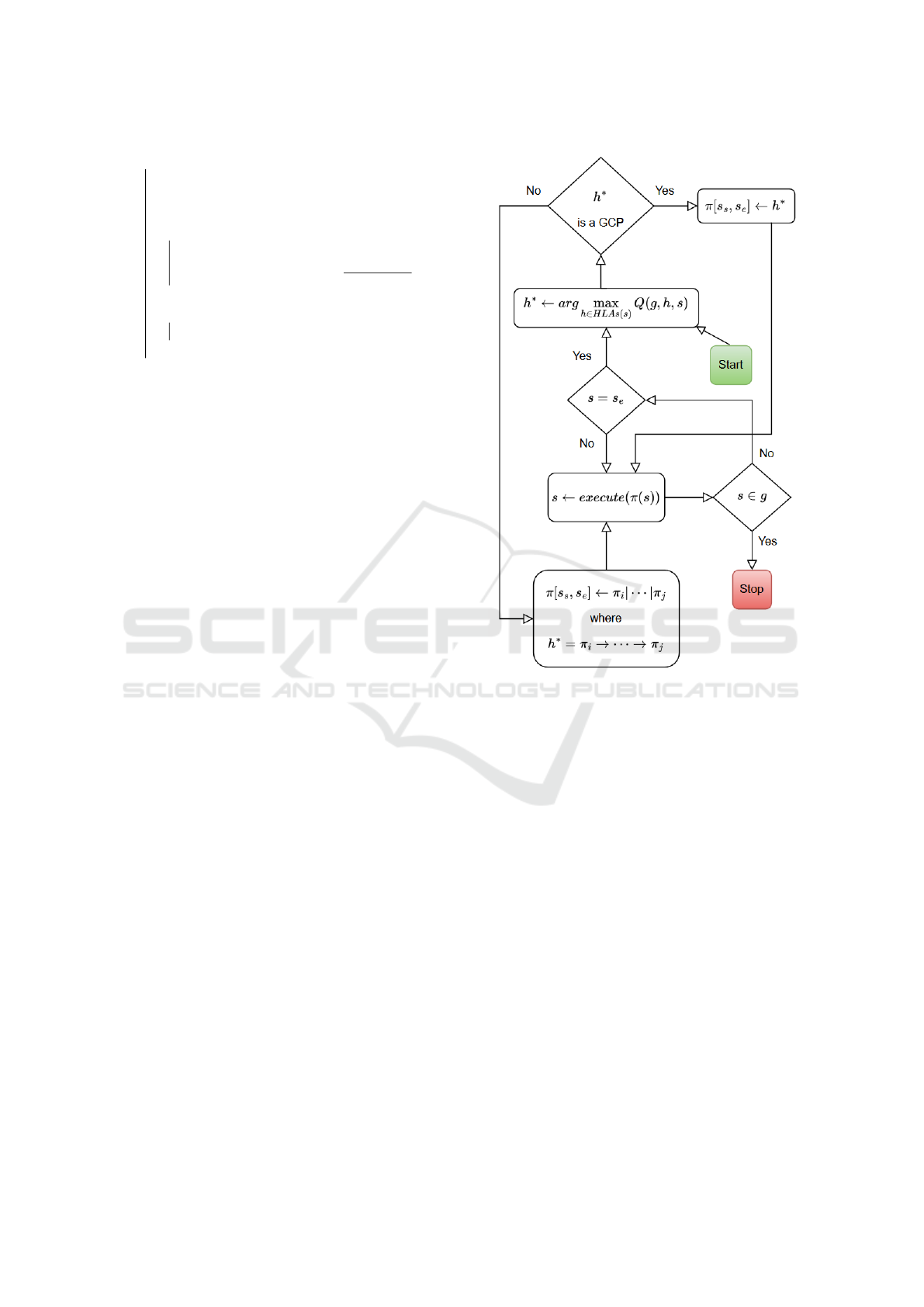
4.7 Executing a Task
Once training is finished, the robot can use the gen-
erated plan-tree to achieve any particular goal g ∈ G.
The execution process is depicted in Figure 3. Note
Figure 3: Execution process for a robot to achieve goal g
starting in state s.
that π
1
|π
2
means that GCPs π
1
[s
1
s
,s
1
e
] and π
2
[s
2
s
,s
2
e
]
are concatenated to form π[s
1
s
,s
2
e
]; concatenation is
defined if and only s
1
e
= s
2
s
.
5 DISCUSSION
5.1 Learning
Almost any RL algorithm can be used to learn GCPs,
once generated. They might need to be slightly mod-
ified to fit the GCRL setting. For instance, Kulkarni
et al. (2016); Zadem et al. (2023) use DQN (Mnih
et al., 2015), Ecoffet et al. (2021) uses PPO (Schul-
man et al., 2017), Yang et al. (2022) uses DDPG (Lil-
licrap et al., 2016) and Shin and Kim (2023); Castanet
et al. (2023) use SAC (Haarnoja et al., 2018).
5.2 Representation of Functions
The three main functions that have to be represented
are the contextual goal-conditioned policies (GCPs),
ICAART 2025 - 17th International Conference on Agents and Artificial Intelligence
512

GCP values and goal-conditioned Q functions. We
propose to approximate these functions with neural
networks.
In the following, we assume that every state s is
described by a set of features, that is, a feature vector
F
s
. Recall that a GCP π[s
s
,s
e
] has context state s
s
and
bev-goal state s
e
. Hence, every GCP can be identified
by its context and bev-goal.
There could be one policy network for all GCPs
π[·,·] that takes as input three feature vectors: a pair
of vectors to identify the GCP and one vector to iden-
tify the state for which an action recommendation is
sought. The output is a probability distribution over
actions A; the output layer thus has |A| nodes. The
action to execute is sampled from this distribution.
There could be one policy-value network for all
R
π
g
that takes as input three feature vectors: a pair of
vectors to identify the GCP and one vector to iden-
tify the state representing the desired goal in G. The
output is a single node for a real number.
There could be one q-value network for Q(h,s, g)
that takes as input four feature vectors: a pair of vec-
tors to identify the HLA h, one vector to identify the
state s and one vector to identify the state representing
the desired goal g ∈ G. The output is a single node for
a real number.
5.3 Memory
“Experience replay was first introduced by Lin (1992)
and applied in the Deep-Q-Network (DQN) algorithm
later on by Mnih et al. (2015).” (Zhang and Sutton,
2017) Archiving or memorizing a selection of trajec-
tories experienced in a replay buffer is employed in
most of the algorithms cited in this paper. Maintain-
ing such a memory buffer in HGCPP would be useful
for periodically updating ChooseBevGoal(·) and the
GCP policy network. We leave the details and inte-
gration into the high-level HGCPP algorithm for fu-
ture work. Also on the topic of memory, we could
generalize the application of generated (remembered)
HLAs: Instead of associating each HLA with a plan-
tree node, we associate them with a state. In this way,
HLAs can be reused from different nodes represent-
ing equal or similar states.
5.4 Opportunism
Suppose we are attempting to learn π[s,s
′
]. If no tra-
jectory starting in s reached s
′
after a given learning-
budget, then instead of placing π[s,s
′
] in HLAs(s),
π[s,s
′′′
] is placed in HLAs(s), where s
′′′
was reached
in at least one experienced trajectory (starting in s)
and is the best (in terms of ChooseBevGoal(·)) of all
states reached while attempting to learn π[s,s
′
]. In the
formal algorithm (line 3.d.) s
′′
is either s
′
or s
′′′
. This
idea of relabeling failed attempts as successful is in-
spired by the Hindsight Experience Replay algorithm
(Andrychowicz et al., 2017).
REFERENCES
Andrychowicz, M., Wolski, F., Ray, A., Schneider, J., Fong,
R., Welinder, P., McGrew, B., Tobin, J., Abbeel, P.,
and Zaremba, W. (2017). Hindsight experience re-
play. In Advances in neural information processing
systems, pages 5048–5058.
Browne, C., Powley, E., Whitehouse, D., Lucas, S., Cowl-
ing, P., Tavener, S., Perez, D., Samothrakis, S., and
Colton, S. (2012). A survey of Monte Carlo tree
search methods. IEEE Transactions on Computa-
tional Intelligence and AI.
Castanet, N., Sigaud, O., and Lamprier, S. (2023). Stein
variational goal generation for adaptive exploration in
multi-goal reinforcement learning. In Proceedings of
the 40th International Conference on Machine Learn-
ing, volume 202. PMLR.
Colas, C., Karch, T., Sigaud, O., and Oudeyer, P.-Y. (2022).
Autotelic agents with intrinsically motivated goal-
conditioned reinforcement learning: A short survey.
Artificial Intelligence Research, 74:1159–1199.
Conti, E., Madhavan, V., Such, F. P., Lehman, J., Stanley,
K. O., and Clune, J. (2017). Improving exploration
in evolution strategies for deep reinforcement learn-
ing via a population of novelty-seeking agents. In
32nd Conference on Neural Information Processing
Systems (NeurIPS 2018).
Ecoffet, A., Huizinga, J., Lehman, J., Stanley, K., and
Clune, J. (2021). First return, then explore”: First re-
turn, then explore. Nature, (590):580–586.
Fang, K., Yin, P., Nair, A., and Levine, S. (2022). Planning
to practice: Efficient online fine-tuning by composing
goals in latent space. In IEEE/RSJ International Con-
ference on Intelligent Robots and Systems (IROS).
Haarnoja, T., Zhou, A., Abbeel, P., and Levine, S. (2018).
Soft actor-critic: Offpolicy maximum entropy deep re-
inforcement learning with a stochastic actor. In Inter-
national conference on machine learning, volume 80,
pages 1861–1870. PMLR.
Hengst, B. (2012). Hierarchical approaches. In Rein-
forcement Learning: State-of-the-Art, volume 12 of
Adaptation, Learning, and Optimization, chapter 9.
Springer.
Hu, W., Wang, H., He, M., and Wang, N. (2023).
Uncertainty-aware hierarchical reinforcement learn-
ing for long-horizon tasks. Applied Intelligence,
53:28555–28569.
Huang, Z., Liu, F., and Su, H. (2019). Mapping state space
using landmarks for universal goal reaching. In 33rd
Conference on Neural Information Processing Sys-
tems (NeurIPS 2019), volume 32, pages 1942–1952.
Proposing Hierarchical Goal-Conditioned Policy Planning in Multi-Goal Reinforcement Learning
513

Khazatsky, A., Nair, A., Jing, D., and Levine, S. (2021).
What can i do here? learning new skills by imagin-
ing visual affordances. In International Conference
on Robotics and Automation (ICRA), pages 14291–
14297. IEEE.
Kocsis, L. and Szepesvari, C. (2006). Bandit based monte-
carlo planning. In European Conference on Machine
Learning.
Kulkarni, T. D., Narasimhan, K. R., Saeedi, A., and Tenen-
baum, J. B. (2016). Hierarchical deep reinforcement
learning: Integrating temporal abstraction and intrin-
sic motivation. In 30th Conference on Neural Infor-
mation Processing Systems (NIPS 2016).
Lehman, J. and Stanley, K. O. (2011). Novelty search and
the problem with objectives. In Genetic Programming
Theory and Practice IX (GPTP 2011).
Li, J., Tang, C., Tomizuka, M., and Zhan, W. (2022). Hi-
erarchical planning through goal-conditioned offline
reinforcement learning. In Robotics and Automation
Letters, volume 7. IEEE.
Li, W., Wang, X., Jin, B., and Zha, H. (2023). Hierarchi-
cal diffusion for offline decision making. In Proceed-
ings of the 40th International Conference on Machine
Learning, volume 202, pages 20035–20064. PMLR.
Lillicrap, T. P., Hunt, J. J., Pritzel, A., Heess, N., Erez, T.,
Tassa, Y., Silver, D., and Wierstra, D. (2016). Contin-
uous control with deep reinforcement learning. In In-
ternational Conference on Learning Representations
(ICLR).
Lin, L.-H. (1992). Self-improving reactive agents based on
reinforcement learning, planning and teaching. Ma-
chine learning, 8(3/4):69–97.
Liu, M., Zhu, M., and Zhangy, W. (2022). Goal-conditioned
reinforcement learning: Problems and solutions. In
Proceedings of the Thirty-First International Joint
Conference on Artificial Intelligence (IJCAI-22).
Lu, L., Zhang, W., Gu, X., Ji, X., and Chen, J. (2020).
Hmcts-op: Hierarchical mcts based online planning
in the asymmetric adversarial environment. Symme-
try, 12(5):719.
Mezghani, L., Sukhbaatar, S., Bojanowski, P., Lazaric, A.,
and Alahari, K. (2022). Learning goal-conditioned
policies offline with self-supervised reward shaping.
In 6th Conference on Robot Learning (CoRL 2022).
Mnih, V., Kavukcuoglu, K., Silver, D., Rusu, A. A., Veness,
J., Bellemare, M. G., Graves, A., and Riedmiller, M.
(2015). Human-level control through deep reinforce-
ment learning. Nature, 518(7540):529–533.
Pertsch, K., Rybkin, O., Ebert, F., Finn, C., Jayaraman,
D., and Levine, S. (2020). Long-horizon visual plan-
ning with goal-conditioned hierarchical predictors. In
34th Conference on Neural Information Processing
Systems (NeurIPS 2020).
Pinto, I. P. and Coutinho, L. R. (2019). Hierarchical re-
inforcement learning with monte carlo tree search
in computer fighting game. IEEE Transactions on
Games, 11(3):290–295.
Plaat, A. (2023). Deep Reinforcement Learning. Springer
Nature.
Schaul, T., Horgan, D., Gregor, K., and Silver, D. (2015).
Universal value function approximators. In Proceed-
ings of ICML-15, volume 37, pages 1312–1320.
Schmidhuber, J. (1991). Curious model-building control
systems. In Proceedings of Neural Networks, 1991
IEEE International Joint Conference, pages 1458–
1463.
Schmidhuber, J. (2006). Developmental robotics, optimal
artificial curiosity, creativity, music, and the fine arts.
Connect. Sci., 18:173–187.
Schulman, J., Wolski, F., Dhariwal, P., Radford, A., and
Klimov, O. (2017). Proximal policy optimization al-
gorithms. CoRR, abs/1707.06347.
Shin, W. and Kim, Y. (2023). Guide to control: Of-
fline hierarchical reinforcement learning using sub-
goal generation for long-horizon and sparse-reward
tasks. In Proceedings of the Thirty-Second Inter-
national Joint Conference on Artificial Intelligence
(IJCAI-23), pages 4217–4225.
Sutton, R. S., Precup, D., and Singh, S. P. (1999). Be-
tween mdps and semi-mdps: A framework for tem-
poral anstraction in reinforcement learning. Artificial
Intelligence, 112(1-2):181–211.
Vassilvitskii, S. and Arthur, D. (2006). k-means++: The
advantages of careful seeding. In Proceedings of the
eighteenth annual ACM-SIAM symposium on discrete
algorithms, page 1027–1035.
Wang, V. H., Wang, T., Yang, W., K am ar ainen, J.-K., and
Pajarinen, J. (2024). Probabilistic subgoal representa-
tions for hierarchical reinforcement learning. In Pro-
ceedings of the 41st International Conference on Ma-
chine Learning, volume 235. PMLR.
Yang, X., Ji, Z., Wu, J., Lai, Y.-K., Wei, C., Liu, G., and
Setchi, R. (2022). Hierarchical reinforcement learning
with universal policies for multi-step robotic manipu-
lation. IEEE Transactions on Neural Networks and
Learning Systems, 33(9):4727–4741.
Zadem, M., Mover, S., and Nguyen, S. M. (2023). Goal
space abstraction in hierarchical reinforcement learn-
ing via set-based reachability analysis. In 22nd IEEE
International Conference on Development and Learn-
ing (ICDL 2023), pages 423–428.
Zhang, S. and Sutton, R. S. (2017). A deeper look at expe-
rience replay. In 31st Conference on Neural Informa-
tion Processing Systems (NIPS 2017).
ICAART 2025 - 17th International Conference on Agents and Artificial Intelligence
514