
Surface Tracking in Coherence Scanning Interferometry by B-Spline
Model and Teager-Kaiser Operator
Fabien Salzenstein
1
, Hassan Mortada
2
, Vincent Mazet
3
and Manuel Flury
4
1
Universit
´
e de Strasbourg, Laboratoire ICube, 23 Rue du Loess, Strasbourg, 67037 Cedex 2, France
2
Exail Technologie, 34 rue de la Croix de fer, Saint Germain en Laye, 78100, France
3
Telecom Physique Strasbourg, Laboratoire ICube, 300 Bd Sbastien Brant, 67400, Illkirch-Graffenstaden, France
4
Institut National des Sciences Appliqu
´
ees, Laboratoire ICube, 24 Bd de la Victoire, Strasbourg, 67000, France
fl
Keywords:
AM-FM Model, B-Spline, Teager-Kaiser Energy Operator, Surface Extraction.
Abstract:
This work deals with the challenge of surface extraction using a combination of Teager-Kaiser operators and B-
splines in the context of coherence scanning (or white light scanning i.e, WLSI) interferometry. Our approach
defines a B-spline regularization model along surface profiles extracting their features by means of parameters
locally describing fringe signals along the optical axis, while most studies are limited to a one-dimensional
signal extraction. In doing so, we take into account four characteristic parameters under Gaussian hypothesis.
The interest of the proposed strategy consists in processing the layers present in a material, in a context of soft
roughness surfaces. The efficiency of our unsupervised method is illustrated on synthetic as well on real data.
1 INTRODUCTION
1.1 Context
White light scanning interferometry (WLSI) is a tech-
nique for analyzing material surfaces, particularly to
estimate their roughness or shape. It can supplement
the manufacturing control of new materials, micro-
electronic devices and microelectromechanical sys-
tems (MEMS) (O’Mahony et al., 2003). In addition,
methods based on the AM-FM model of the inter-
ference signal along the optical axis allow an accu-
rate precision. Thus, the information about the depth
of the material can be extracted simultaneously from
the envelope and the phase of the AM-FM signal.
Plenty of algorithms, whether based on envelope de-
tection (Larkin, 1996; Sandoz, 1997), frequency do-
main analysis (de Groot and Deck, 1993; de Groot
et al., 2002), correlation with a reference fringe (Chim
and Kino, 1990), Hilbert transformation (Pavli
ˇ
cek
and Michalek, 2012), TK algorithm (Gianto et al.,
2016), extraction of the phase information (Guo et al.,
2011), Kalman approach (Gurov et al., 2004), have
been proposed, proceeding along the optical axis i.e,
thus corresponding to 1D approach. Additionally 2D
techniques have been presented (Gurov and Volynsky,
2012; Zhu and Wang, 2012). Due to its simplicity of
implementation, adapted to the AM-FM signal model,
the nonlinear Teager-Kaiser energy operator (TK or
TKEO) (Vakman D., 1996; Maragos P. et al., 1993)
seems to be effective (Larkin, 1996; Salzenstein et al.,
2014) as well in its bi-dimensional (Boudraa et al.,
2005) or multidimensional version (Salzenstein and
Boudraa, 2009). In particular, most of these meth-
ods undertake to measure the roughness of surfaces,
namely the evolution of their depth according to the
lateral directions. We believe that approaches, which
may take into account both lateral and height informa-
tion, namely 2D or even 3D processing over the en-
tire data cube, are potentially more suitable than one-
dimensional approaches, in order to track surfaces, es-
pecially when they own low roughness. Our study fo-
cuses on a new 2D method, adapted for such surfaces.
1.2 Objectives
In order to ensure a good surface tracking, taking into
account the neighborhood information along the lat-
eral axis, by a regularization approach, we propose
to describe four characteristic parameters of AM-FM
signals under the hypothesis of a Gaussian envelope,
by introducing a B-spline modeling, combined with
the TK operator. A study based on spectral tracking
has been carried out in the field of astronomy, pro-
Salzenstein, F., Mortada, H., Mazet, V. and Flury, M.
Surface Tracking in Coherence Scanning Interferometry by B-Spline Model and Teager-Kaiser Operator.
DOI: 10.5220/0013239700003905
In Proceedings of the 14th International Conference on Pattern Recognition Applications and Methods (ICPRAM 2025), pages 681-688
ISBN: 978-989-758-730-6; ISSN: 2184-4313
Copyright © 2025 by Paper published under CC license (CC BY-NC-ND 4.0)
681

viding solutions to close problems (considering spec-
tral data) although signals do not contain any carrier
term (Mortada et al., 2018). B-splines have proven
their effectiveness in many areas of signal processing.
One of their common applications consists in interpo-
lation (Reinsch, 1967; Unser, 1999), which is helpful
to find pixel values at continuous positions after some
geometric transformations, for image resizing and re-
sampling. They have also found other application in
image registration (Rueckert et al., 2006), edge de-
tection (Mallat and Zhong, 1992), signal compression
(Medioni and Yasumoto, 1987), 3D modeling (Hoch
et al., 1994). In the field of coherence scanning in-
terferometry, this approach has been helpful to im-
prove the interference signal (Duan et al., 2023) on
the optical axis (depth) in the context of least squares
phase shift methods (as well for continuous phase es-
timation related to the noisy fringe patterns in digi-
tal speckle interferometry (Wielgus et al., 2014)) or
to approximate local detected envelope (Montgomery
et al., 2013). B-spline technique has been proposed to
fit surfaces, without taking into account the physical
local model of the interference signal (Bruno, 2007).
To the best of our knowledge, no global approach has
been proposed modeling four characteristic parame-
ters (surface position, amplitude, variance, carrier fre-
quency) by B-splines, under the assumption of locally
Gaussian envelopes: this deals with the main contri-
butions of our study, in combination with a TK tech-
nique. The remainder of the paper is organized as
follows: after the presentation of the context of the
interferometric data in section 2 we recall TK algo-
rithm and B-spline approach, respectively in section
3 and 4. An unsupervised model adapted to our data
has been detailed in section 5. Finally, results on both
synthetic and real images are presented in section 6.
2 INTERFEROMETRIC SIGNAL
Figure 1 shows the typical layout of WLSI device us-
ing the z-scan technique. By means of a single ver-
tical scan of the sample, over the whole depth of the
surface by modifying the distance between the objec-
tive and the sample, a stack of xyz images is pro-
duced. The resulting signal corresponds to the sum
of the interferences at each wavelength. From such
a signal, the objective is to extract depth information
related to the analyzed surfaces. For surface rough-
ness measurement, a classic signal processing tech-
nique generally aims to provide position at the max-
imum of the single fringe envelope along the depth
handled by the optical axis z for each lateral coordi-
nate (x, y), which represents the horizontal extent of
a material sample. Therefore, the (relatively) greater
the variation in surface height between neighboring
lateral sites, the rougher it will be considered.
Figure 1: Schematic layout of WLSI system. The right hand
pattern represents an interference signal along the depth
axis z for two layers of surfaces, at a given (x,y) position.
Figure 2: Recovery and process of a 2D xz image from a 3D
xyz block generated by the WLSI interferometric system.
A typical intensity signal obtained from a digital
camera when the OPD (optical path difference) varies
in the interferometer at a given point (x,y) on the ma-
terial surface, can be approximated along the optical
z axis by a such modulated sinusoid (Larkin, 1996):
s(x,y,z) = a(x,y,z) + b(x,y) exp
"
−
z − h(x,y)
l
c
2
#
| {z }
C(x,y,z)
×cos
4π
λ
0
(z − h(x,y)) + α(x,y)
where z is a vertical scanning position along the op-
tical axis, h(x,y) represents the height of the sur-
face, a(x,y,z) is an offset intensity containing low fre-
quency components, b(x,y) is a factor proportional to
the reflected beam intensity, and α(x,y) is an addi-
tional phase offset and C(x,y,z) is the envelope. The
parameter l
c
represents the coherence length and λ
0
,
the average wavelength of the light source. Generally
the phase offset varies slowly from one point (x,y)
to the next, and can be neglected, since only rela-
tive heights of the surface matter. The main chal-
lenge consists in determining the height at each point
of the surface by exploiting the information provided
by both the envelope or the phase simultaneously.
ICPRAM 2025 - 14th International Conference on Pattern Recognition Applications and Methods
682

3 TEAGER-KAISER ENERGY
OPERATORS
TKEOs algorithms (Boudraa and Salzenstein, 2018)
are non-linear methods for envelope detection and
phase retrieval from AM-FM signals such as those
given by Eq. (1). For a such given signal s(t), the
output of the continuous TKEO, denoted by Ψ, yields
the following expression (Maragos P. et al., 1993):
Ψ[s(t)] = [ ˙s(t)]
2
− s(t) ¨s(t) (1)
where ˙s(t) and ¨s(t) denote the first and the second
time derivatives of s(t) respectively. Under realistic
conditions (Maragos et al., 1993), when applied to
AM-FM signal s(t) = a(t)cos(φ(t)), the 1D TKEO
yields as output Ψ[s(t)] ≈ [a(t)
˙
φ(t)]
2
. Thus the local
envelope a(t) and the instantaneous frequency
˙
φ(t)
can be estimated using the energy separation algo-
rithm (ESA) (Maragos et al., 1993):
|
˙
φ(t)| ≈
s
Ψ[ ˙s(t)]
Ψ[s(t)]
; |a(t)| ≈
Ψ[s(t)]
p
Ψ[ ˙s(t)]
(2)
A discrete TKEO, applied to a differentiated sig-
nal, called FSA, has been used in WSLI (Larkin,
1996). This operator, as well useful for n-D de-
modulation, has been extended to multidimensional
signals (Maragos and Bovik, 1995; Boudraa et al.,
2005; Larkin, 2005), also using directional deriva-
tives (Salzenstein et al., 2013). It can be effective to
improve the fineness of the information, by combin-
ing other approaches, such as a correlation technique
(Salzenstein et al., 2014). In this study, we exploit
TKEO, in order to initialize our B-spline estimation
algorithm.
4 SUMMARY OF THE B-SPLINE
MODEL
We propose to model the surface parameters by B-
splines. This piecewise polynomial approach was in-
troduced in (Schoenberg, 1946). The linear combina-
tion of these functions allows to express a continuous
function with a countable set of variables, called con-
trol points. Defining the set of B-spline basis func-
tions require two elements:
• a degree d (or order d + 1), that specifies the max-
imal degree of the polynomial functions;
• a knot vector k that is a sequence of increas-
ing real numbers, i.e., k =
{
k
0
,k
1
,k
K
}
, with k
0
≤
k
1
... ≤ k
K
.
Considering K + 1 nodes, a polynomial function
of degree d is defined between two consecutive nodes.
A B-spline basis function of degree d comprises d +2
consecutive nodes from the vector k. The number of
B-spline basis functions of degree d is thus equal to
M = K − d. Let b
d
m
(x), where m ∈
{
1,...,M
}
, be the
mth B-spline basis function of degree d defined on
k
m
,...,k
m+d+1
for a given variable x. The Cox de Boor
algorithm (De Boor, 1972), generates B-spline basis
by recurrence formula:
b
0
m
(x) =
(
1 if k
m
≤ x < k
m+1
0 otherwise
b
d
m
(x) =
x − k
m
k
m+d
− k
m
b
d−1
m
(x) +
k
m+d+1
− x
k
m+d+1
− k
m+1
b
d−1
m+1
(x)
An alternative method consist in applying d convolu-
tion, such that:
b
d
m
(x) = b
0
m
∗ b
0
m
∗ ... ∗ b
0
m
| {z }
d times
(x)
Among the remarkable properties of B-splines, let
us highlight i) locality of their support i.e, b
d
m
(x) =
0 ∀ x /∈ [k
m
,k
m+d+1
]; ii) nullity of the values at extrem-
ities of their interval i.e, b
d
m
(k
m
) = b
d
m
(k
m+d+1
) = 0;
iii) non negativity i.e, ∀x b
d
m
(x) ≥ 0; iv) normalized
sum for non-zero functions on a knot interval i.e.,
∑
M
m=1
b
d
m
(x) = 1 ∀ x ∈ [k
m
,k
m+1
]; v) B-spline functions
are related to C
d
class of continuity, on a knot in-
terval [k
m
,k
m+d+1
]. A uniform knot vector, formed
by equally spaced knots, helps to provide B-spline
basis functions as shifted versions of each others:
∀ m ∈
{
1,2,..., M
}
,b
d
m
(x) = b
d
0
(x − k
m
). It is possible
to construct B-spline functions M = K − d of degree
d, defined on a vector of knots containing K + 1 ele-
ments, taking into account the knots coinciding at the
extremities.
5 B-SPLINE MODEL OF
INTERFEROMETRIC SIGNAL
CHARACTERISTICS
An interpolation or approximation problem yields to
a B-spline curve f (x) expressed in the following way:
f (x) =
M
∑
m=1
u
m
b
d
m
(x), (3)
where u
m
∈ R is a control point (called also ’weights’)
of the mth B-spline basis function b
d
m
(x). Given
b[x] =
b
d
1
(x) b
d
2
(x) ... b
d
M
(x)
T
and u = [u
1
...u
M
] Eq.
(3) yields to a vector characterization:
f (x) = b [x]
T
u (4)
Surface Tracking in Coherence Scanning Interferometry by B-Spline Model and Teager-Kaiser Operator
683

We process the volume of data, described in sec-
tion 2 by proceeding slice by slice, corresponding to
2D signals s(z,i), denoted by s
i
(z), say of size N × I
where N is the length of the optical axis (commonly
called z-axis) and I is the maximum size of the lat-
eral axis i (commonly called x-axis). For a given set
of J surfaces or layers of material, an interferometric
model may be expressed in a following way by con-
sidering an additive noise n
i
(z)
s
i
(z) =
J
∑
j=1
a
i j
exp
"
−
(z − c
i j
)
2
2σ
2
i j
#
×cos (2πν
i j
(z − c
i j
)) + n
i
(z)
which could be condensed using a parametric func-
tion φ, including Gaussian and carrier, as follows:
s
i
(z) =
J
∑
j=1
a
i j
φ(z − c
i j
;σ
i j
;ν
i j
) + n
i
(z) (5)
Hence, each surface of the material, labeled
by j could be estimated by a set of centers
{
c
1 j
,c
2 j
,...,c
I j
}
. In other words, for each lateral po-
sition i the peak related to a class j is parameterized
along the optical axis z, by its center c
i j
, amplitude
a
i j
and standard deviation σ
i j
, at a given carrier fre-
quency ν
i j
. This is summed up in a vectorized form:
s
i
=
J
∑
j=1
a
i j
Φ(c
i j
;σ
i j
;ν
i j
) + n
i
(6)
In our model, extended (Mortada et al., 2018), un-
der an assumption of locally smooth surfaces, we as-
sume that all characteristic parameters c
i j
, a
i j
, σ
i j
,
ν
i j
parameters are modeled by B-splines defined on
the same knot vector k, with unknown control points.
Considering knot positions on discrete values, yields:
∀ j, a
i j
= a
j
(i) =
M
∑
m=1
A
j
m
b
d
m
(i) = b[i]
T
A
j
(7)
∀ j, c
i j
= c
j
(i) =
M
∑
m=1
C
j
m
b
d
m
(i) = b[i]
T
C
j
(8)
∀ j, σ
i j
= σ
j
(i) =
M
∑
m=1
Σ
j
m
b
d
m
(i) = b[i]
T
Σ
j
(9)
∀ j, ν
i j
= ν
j
(i) =
M
∑
m=1
V
j
m
b
d
m
(i) = b[i]
T
V
j
(10)
where A =
h
A
j
1
,A
j
2
,...,A
j
M
i
T
, C, Σ, V respectively de-
fine the control points related to the amplitude, sur-
face position, gaussian shape and carrier frequency,
whereas b[i]
T
=
b
d
1
(i) b
d
2
(i) ...
being a vector gath-
ering the B-splines evaluated at the mixture index i.
Finally, the proposed model approximating the inter-
ferometric signal s
i
by means of B-splines becomes:
∀i,s
i
=
J
∑
j=1
b[i]
T
A
j
Φ
b[i]
T
;C
j
;Σ
j
;V
j
+ n
i
(11)
Under Gaussian noisy assumption, the maximum
likelihood estimation of the control points parameters,
leads to the minimization of the following function:
L (Θ) =
∑
i
s
i
−
J
∑
j=1
b[i]
T
A
j
Φ
b[i]
T
;C
j
;Σ
j
;V
j
2
where Θ = (A,C,Σ, V). In order to solve the non-
linear least square minimization problem min
Θ
L (Θ),
as in (Mortada et al., 2018), a Sequential Quadratic
Programming (SQP) algorithm (Nocedal and Wright,
1999) could be helpful. However, to enhance robust-
ness in certain situations we have tested (synthetic
and real data), a classic simulated annealing algo-
rithm, moving the control points, proves its effective-
ness. We have implemented it, in combination with
the Teager-Kaiser to enhance parameter initialization.
6 RESULTS
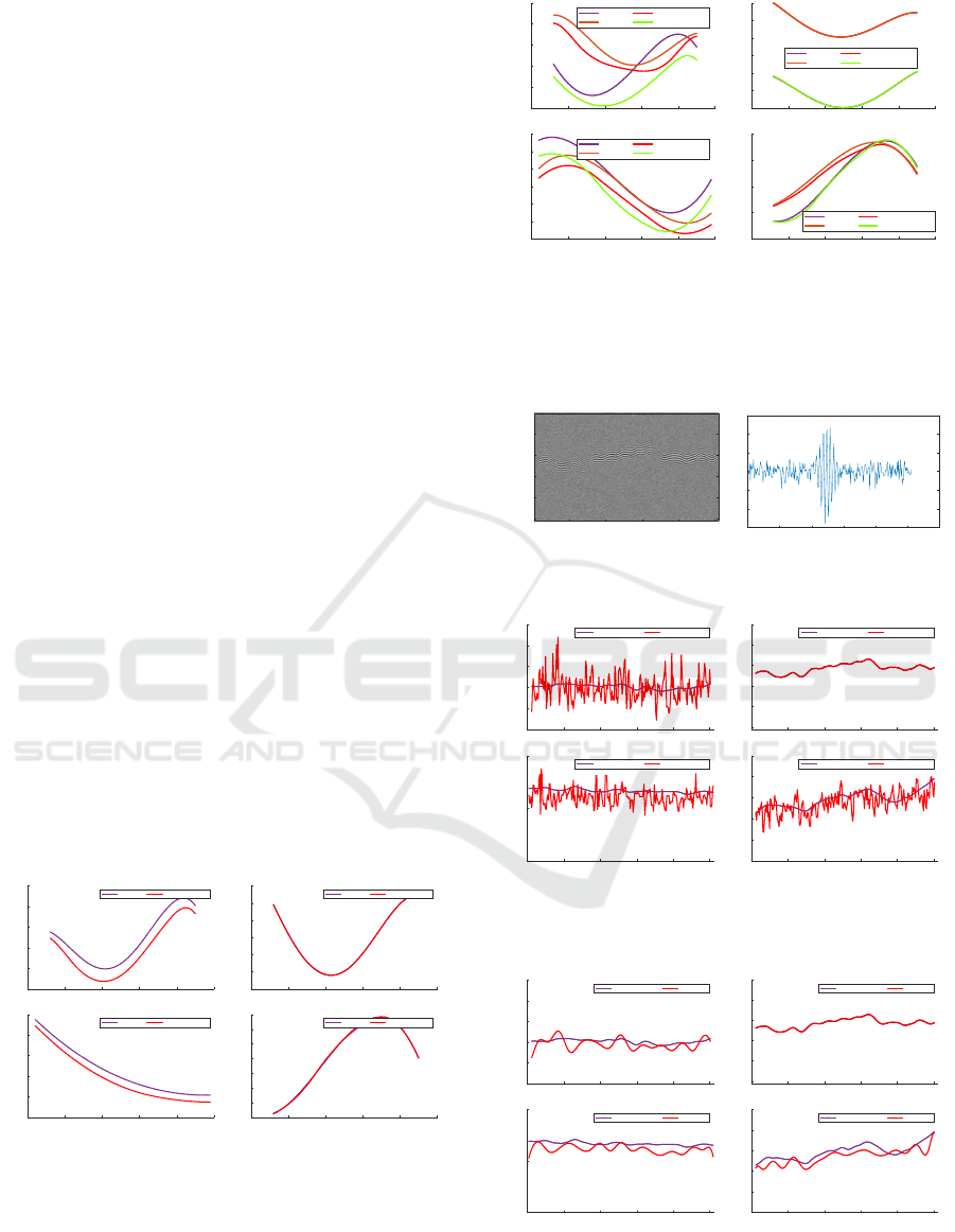
6.1 Synthetic Data and Images
We illustrate the proposed model and its robustness on
synthetic data, synthetic and real interferometric im-
ages. Fig. 3-4 show initial and estimated data related
to the four parameters of interest, for a signal-to-noise
ratio of 20 dB, respectively in the context of one class
and two classes, by the method SQP. The number of
control points respectively equals 7,6,7, 6 concern-
ing the surfaces, amplitudes, variances, and frequen-
cies. These examples make relevant the possibility of
exploiting B-splines by means of our interferometric
model. Fig. 5,6,7,8,9,10 deal with synthetic interfero-
metric images and their estimates, for which the initial
data were simulated by smoothing randomly initial
data (produced by stochastic process). In a context
of relatively low SNR (5 dB), the quantitative perfor-
mances of the Teager-Kaiser method and B-Splines
are reported in tables 1 and 2. We have processed
Teager-Kaiser technique to initialize our method, fol-
lowed by a simulated annealing approach. The com-
bination of both techniques allows a better conver-
gence of the algorithm, while improving the estima-
tion for all characteristic parameters. The number of
control points is respectively 41 for estimating the
surfaces, and 21 for the other parameters. In partic-
ular, the algorithm based on B-splines significantly
reduces the error rate of variances and frequencies,
which shows, in this context, that regularization tak-
ing into account neighboring information over all the
parameters, contributes to a better estimation of the
surface.
ICPRAM 2025 - 14th International Conference on Pattern Recognition Applications and Methods
684
6.2 Real Interferometric Images
Finally, as illustrated in Fig.11, Fig.12 we have ap-
plied the previous algorithm to real interferometric
images. Fig.11 shows a silicon surface that both al-
gorithms process in a relatively similar manner, the
B-spline method estimating the frequencies better (in
the real image, these are much more continuous than
the TK algorithm suggests) and, as expected, slightly
smoothing the data produced by TKEO. Each param-
eter is estimated using P = 36 control points. Let us
note the relatively high noise level by observing the
profile Fig.11(b). Fig.12 shows the effectiveness of
the method applied to the detection of a oil drop, for
which certain areas of the image, very noisy, make the
Teager-Kaiser algorithm almost inoperative. The re-
sulting surface of the B-spline approach corrects this
drawback, and perfectly matches the shape of the oil-
drop. Under a relevant assumption, the carrier fre-
quency fluctuating quite little, the order of the B-
spline regarding frequencies was set to 3 (second or-
der polynomial). This allows us to obtain a more sta-
ble estimate than the TKEO. On the other hand, both
approaches determine a decreasing amplitude (the ap-
pearance of the oil-drop interference signal being em-
pirically attenuated in the right part of the image),
which makes it compatible, at constant frequency,
with an increasing variance (spreading out Gaussian
envelope). Finally, the relative small number of con-
trol points (8 for surface, amplitude and variance, 6
for frequency) seems appropriate for this very smooth
surface. Finally, let us note that the average calcula-
tion time for an 256x256 image corresponds to 15 sec-
onds (Matlab2022, cpu Intel Core i5-7300U 2.6 GHz,
Ram 16Go).
0 10 20 30 40 50
Original and estimated frequencies
5
5.1
5.2
5.3
5.4
5.5
Class 1 Estim Class 1
0 10 20 30 40 50
Original and estimated surfaces
140
150
160
170
180
190
200
Class 1 Estim Class 1
0 10 20 30 40 50
Original and estimated amplitudes
2
2.5
3
3.5
4
4.5
5
5.5
Class 1 Estim Class 1
0 10 20 30 40 50
Original and estimated variances
5
5.2
5.4
5.6
5.8
6
Class 1 Estim Class 1
(a)
Figure 3: (a): One class data (in blue) and their
estimation (in red) by cubic B-spline (variance, sur-
face, frequency, amplitude) with knot vector k =
[1,1,1,1,1.7,20.5,30.2, 50, 50, 50, 50]; the number of con-
trol points being respectively 7, 6, 7, 6.
0 10 20 30 40 50
Original and estimated frequencies
5.1
5.15
5.2
5.25
5.3
5.35
5.4
Class 1
Class 2
Estim Class 2
Estim Class 1
0 10 20 30 40 50
Original and estimated surfaces
100
120
140
160
180
200
220
Class 1
Class 2
Estim Class 2
Estim Class 1
0 10 20 30 40 50
Original and estimated amplitudes
0
2
4
6
8
Class 1
Class 2
Estim Class 2
Estim Class 1
0 10 20 30 40 50
Original and estimated variances
5
5.2
5.4
5.6
5.8
6
Class 1
Class 2
Estim Class 2
Estim Class 1
(a)
Figure 4: (a): Two classes data (resp. in purple and
brown) and their estimation (resp. in green and red) by cu-
bic B-spline (variance, surface, frequency, amplitude) with
knot vector k = [1,1, 1, 1, 10.7, 20.5, 30.2, 50, 50, 50, 50]; the
number of control points being respectively 7, 6, 7, 6.
50 100 150 200 250
lateral axis x
50
100
150
200
250
optical axis z
0 50 100 150 200 250 300
-30
-20
-10
0
10
20
30
(a) (b)
Figure 5: (a): Synthetic interferometric signal; (b) profile
signal along the optical axis;
0 50 100 150 200 250
Original and estimated frequencies
0.5
1
1.5
Original Class Teager Kaiser
0 50 100 150 200 250
Original and estimated surfaces
0
50
100
150
200
250
Original Class Teager Kaiser
0 50 100 150 200 250
Original and estimated amplitudes
20
22
24
26
28
30
Original Class Teager Kaiser
0 50 100 150 200 250
Original and estimated variances
10
12
14
16
18
20
Original Class Teager Kaiser
Figure 6: original (in blue) and estimated parameters (in
red) of Fig. 5(a) with Teager-Kaiser (from top left to bottom
right: variance, surface, frequency, amplitude).
0 50 100 150 200 250
Original and estimated frequencies
0.5
1
1.5
Original Class B-Spline
0 50 100 150 200 250
Original and estimated surfaces
0
50
100
150
200
250
Original Class B-Spline
0 50 100 150 200 250
Original and estimated amplitudes
20
22
24
26
28
30
Original Class B-Spline
0 50 100 150 200 250
Original and estimated variances
10
12
14
16
18
20
Original Class B-Spline
Figure 7: original (in blue) and estimated parameters (in
red) of Fig. 5(a) with B-Spline technique (from top left to
bottom right: variance, surface, frequency, amplitude).
Surface Tracking in Coherence Scanning Interferometry by B-Spline Model and Teager-Kaiser Operator
685
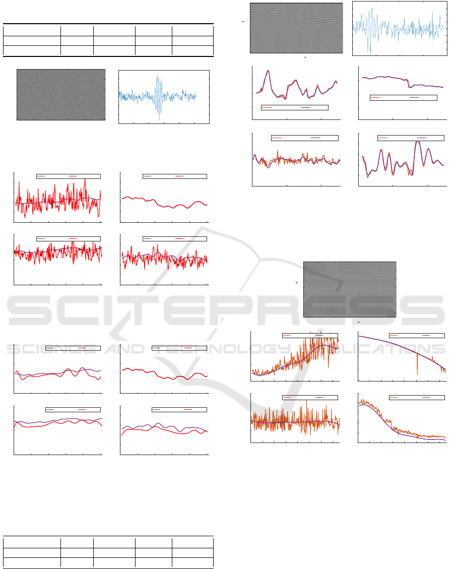
Table 1: Fig. 6, 7 : error rates estimation (%) for each char-
acteristic, for TK alone and then combined with B-Spline.
surface amplitude variance frequency
Teager-Kaiser 0.37 2.63 6.77 6.78
TK + B-Spline 0.27 1.98 2.82 4.37
50 100 150 200 250
lateral axis x
50
100
150
200
250
optical axis z
0 50 100 150 200 250 300
-30
-20
-10
0
10
20
30
(a) (b)
Figure 8: (a): Synthetic interferometric signal; (b) profile
signal along the optical axis; .
0 50 100 150 200 250
Original and estimated frequencies
0.5
1
1.5
Original Class Teager Kaiser
0 50 100 150 200 250
Original and estimated surfaces
0
50
100
150
200
250
Original Class Teager Kaiser
0 50 100 150 200 250
Original and estimated amplitudes
20
22
24
26
28
30
Original Class Teager Kaiser
0 50 100 150 200 250
Original and estimated variances
10
12
14
16
18
20
Original Class Teager Kaiser
Figure 9: original (in blue) and estimated parameters (in
red) of Fig. 8(a) with Teager-Kaiser (from top left to bottom
right: variance, surface, frequency, amplitude).
0 50 100 150 200 250
Original and estimated frequencies
0.5
1
1.5
Original Class B-Spline
0 50 100 150 200 250
Original and estimated surfaces
0
50
100
150
200
250
Original Class B-Spline
0 50 100 150 200 250
Original and estimated amplitudes
20
22
24
26
28
30
Original Class B-Spline
0 50 100 150 200 250
Original and estimated variances
10
12
14
16
18
20
Original Class B-Spline
Figure 10: original (in blue) and estimated parameters (in
red) of Fig. 8(a) with B-Spline technique (from top left to
bottom right: variance, surface, frequency, amplitude).
Table 2: Fig. 9, 10 : error rates estimation (%) for each char-
acteristic, for TK alone and then combined with B-Spline.
surface amplitude variance frequency
Teager-Kaiser 0.53 3.31 8.27 7.68
TK + B-Spline 0.33 2.76 3.77 4.92
Silicium Image
0 10 20 30 40 50
lateral axis x ( m)
0
5
10
15
optical axis z ( m)
0 50 100 150 200
-8
-6
-4
-2
0
2
4
6
8
(a) (b)
0 50 100
estimated frequencies (y-axis in MHz)
0.5
1
1.5
Teager-Kaiser B-Spline
0 50 100
estimated surfaces
0
50
100
150
Teager-Kaiser B-Spline
0 50 100
estimated amplitudes
0
20
40
60
80
100
Teager-Kaiser B-Spline
0 50 100
estimated variances
0
10
20
30
40
Teager-Kaiser B-Spline
(c)
Figure 11: (a): Real interferometric image and its profile
(b) along the optical axis; (c): estimated parameters with B-
Splines (in blue) and Teager-Kaiser (in red): from top left
to bottom right: variance, surface, frequency, amplitude.
Waterdrop Image
0 10 20 30 40 50
lateral axis x ( m)
0
5
10
15
20
25
30
optical axis z ( m)
(a)
0 50 100 150 200 250 300 350
estimated frequencies (y-axis in MHz)
0.5
1
1.5
2
2.5
Teager-Kaiser B-Spline
0 50 100 150 200 250 300 350
estimated surfaces
0
100
200
300
400
Teager-Kaiser B-Spline
0 50 100 150 200 250 300 350
estimated amplitudes
0
2
4
6
8
10
Teager-Kaiser B-Spline
0 50 100 150 200 250 300 350
estimated variances
15
20
25
30
Teager-Kaiser B-Spline
(b)
Figure 12: (a): oil-drop interferometric image; (b): es-
timated parameters with B-Splines (in blue) and Teager-
Kaiser (in red): from top left to bottom right: variance, sur-
face, frequency, amplitude.
7 CONCLUSION
In this paper, we have introduced a new method for
tracking material surfaces, combining two types of
approaches: a nonlinear Teager-Kaiser operator, and
a model based on B-splines, allowing a regulariza-
tion taking into account the neighboring points of
the surface according to four parameters capable of
characterizing a fringe signal. After initialization us-
ICPRAM 2025 - 14th International Conference on Pattern Recognition Applications and Methods
686

ing TKEO, we estimate the control points by a sim-
ulated annealing procedure. Although our assump-
tion is suitable for relatively smooth surfaces, we have
provided promising quantitative and also qualitative
results. We have illustrated the performance of our
method on synthetic and real images, showing its abil-
ity to match the roughness of the surfaces. A possible
extension of our algorithm could concern, on the one
hand, an initialization step (by TKEO or another op-
erator) more adapted to noisy data. On the other hand,
the consideration of other image slices within the 3D
data cube (neighboring xz sections) to help initializa-
tion, and also enrichment of the model by using more
complex splines choosing locally different orders for
each parameter or, for example, using P-spline model.
The relatively fast processing, which can be paral-
lelized (more efficient simulated annealing etc), an
interactive procedure would make it possible to opti-
mize the suitable number of splines. For an automatic
procedure, this number depending on each parameter,
could be based on machine learning adapted to data
similar to those being processed.
ACKNOWLEDGEMENTS
We would like to thank Mr. Freddy Anstotz and Mr.
Christophe Cordier from the IPP laboratory, for pro-
viding the interferometric images.
REFERENCES
Boudraa, A.-O. and Salzenstein, F. (2018). Teager–kaiser
energy methods for signal and image analysis: A re-
view. Digital Signal Processing, 78:338–375.
Boudraa, A.-O., Salzenstein, F., and Cexus, J.-C. (2005).
Two-dimensional continuous higher-order energy op-
erators. Optical Engineering, 44(11):117001–117001.
Bruno, L. (2007). Global approach for fitting 2d interfero-
metric data. Optics Express, 15(8):4835–4847.
Chim, S. S. and Kino, G. S. (1990). Correlation microscope.
Optics Letters, 15(10):579–581.
De Boor, C. (1972). On calculating with b-splines. Journal
of Approximation theory, 6(1):50–62.
de Groot, P., de Lega, X. C., Kramer, J., and Turzhit-
sky, M. (2002). Determination of fringe order in
white-light interference microscopy. Applied optics,
41(22):4571–4578.
de Groot, P. and Deck, L. (1993). Three-dimensional imag-
ing by sub-nyquist sampling of white-light interfero-
grams. Optics Letters, 18(17):1462–1464.
Duan, Y., Li, Z., and Zhang, X. (2023). Least-squares
phase-shifting algorithm of coherence scanning in-
terferometry with windowed b-spline fitting, resam-
pled and subdivided phase points for 3d topography
metrology. Measurement, 217:113103.
Gianto, G., Salzenstein, F., and Montgomery, P. (2016).
Comparison of envelope detection techniques in co-
herence scanning interferometry. Applied Optics,
55(24):6763–6774.
Guo, T., Ma, L., Chen, J., Fu, X., and Hu, X. (2011).
Microelectromechanical systems surface characteri-
zation based on white light phase shifting interferom-
etry. Optical Engineering, 50(5):053606–053606.
Gurov, I., Ermolaeva, E., and Zakharov, A. (2004). Analysis
of low-coherence interference fringes by the kalman
filtering method. Journal of the Optical Society of
America A, 21(2):242–251.
Gurov, I. and Volynsky, M. (2012). Interference fringe anal-
ysis based on recurrence computational algorithms.
Optics and Lasers in Engineering, 50(4):514–521.
Hoch, M., Fleischmann, G., and Girod, B. (1994). Mod-
eling and animation of facial expressions based on b-
splines. The Visual Computer, 11:87–95.
Larkin, K. G. (1996). Efficient nonlinear algorithm for en-
velope detection in white light interferometry. Journal
of the Optical Society of America A, 13(4):832–843.
Larkin, K. G. (2005). Uniform estimation of orientation
using local and nonlocal 2-d energy operators. Optics
Express, 13(20):8097–8121.
Mallat, S. and Zhong, S. (1992). Characterization of signals
from multiscale edges. IEEE Transactions on Pattern
Analysis & Machine Intelligence, 14(07):710–732.
Maragos, P. and Bovik, A. C. (1995). Image demodulation
using multidimensional energy separation. Journal of
the Optical Society of America A, 12(9):1867–1876.
Maragos, P., Kaiser, J. F., and Quatieri, T. F. (1993). Energy
separation in signal modulations with application to
speech analysis. IEEE Transactions on Signal Pro-
cessing, 41(10):3024–3051.
Maragos P., Kaiser J.F., and QuatieriT.F. (1993). On am-
plitude and frequency demodulation using energy op-
erators. IEEE Transactions on Signal Processing,
41(4):1532–1550.
Medioni, G. and Yasumoto, Y. (1987). Corner detection and
curve representation using cubic b-splines. Computer
vision, graphics, and image processing, 39(3):267–
278.
Montgomery, P. C., Salzenstein, F., Montaner, D., Serio, B.,
and Pfeiffer, P. (2013). Implementation of a fringe
visibility based algorithm in coherence scanning in-
terferometry for surface roughness measurement. In
Optical Measurement Systems for Industrial Inspec-
tion VIII, volume 8788, pages 951–961. SPIE.
Mortada, H., Mazet, V., Soussen, C., and Collet, C. (2018).
Spectroscopic decomposition of astronomical multi-
spectral images using b-splines. In 2018 9th Work-
shop on Hyperspectral Image and Signal Processing:
Evolution in Remote Sensing (WHISPERS), pages 1–
5. IEEE.
Nocedal, J. and Wright, S. J. (1999). Numerical optimiza-
tion. Springer.
O’Mahony, C., Hill, M., Brunet, M., Duane, R., and Math-
ewson, A. (2003). Characterization of micromechan-
Surface Tracking in Coherence Scanning Interferometry by B-Spline Model and Teager-Kaiser Operator
687

ical structures using white-light interferometry. Mea-
surement Science and Technology, 14(10):1807.
Pavli
ˇ
cek, P. and Michalek, V. (2012). White-light interfer-
ometryenvelope detection by hilbert transform and in-
fluence of noise. Optics and Lasers in Engineering,
50(8):1063–1068.
Reinsch, C. H. (1967). Smoothing by spline functions. Nu-
merische mathematik, 10(3):177–183.
Rueckert, D., Aljabar, P., Heckemann, R. A., Hajnal, J. V.,
and Hammers, A. (2006). Diffeomorphic registra-
tion using b-splines. In Medical Image Computing
and Computer-Assisted Intervention–MICCAI 2006:
9th International Conference, Copenhagen, Denmark,
October 1-6, 2006. Proceedings, Part II 9, pages 702–
709. Springer.
Salzenstein, F. and Boudraa, A.-O. (2009). Multi-
dimensional higher order differential operators de-
rived from the Teager-Kaiser energy tracking func-
tion. Signal Processing, 89(4):623–640.
Salzenstein, F., Boudraa, A.-O., and Chonavel, T. (2013).
A new class of multi-dimensional teager-kaiser and
higher order operators based on directional deriva-
tives. Multidimensional Systems and Signal Process-
ing, 24:543–572.
Salzenstein, F., Montgomery, P., and Boudraa, A.-O.
(2014). Local frequency and envelope estimation by
teager-kaiser energy operators in white-light scanning
interferometry. Optics Express, 22(15):18325–18334.
Sandoz, P. (1997). Wavelet transform as a processing
tool in white-light interferometry. Optics Letters,
22(14):1065–1067.
Schoenberg, I. J. (1946). Contributions to the problem of
approximation of equidistant data by analytic func-
tions. part b. on the problem of osculatory interpola-
tion. a second class of analytic approximation formu-
lae. Quarterly of Applied Mathematics, 4(2):112–141.
Unser, M. (1999). Splines: A perfect fit for signal and im-
age processing. IEEE Signal processing magazine,
16(6):22–38.
Vakman D. (1996). On the analytic signal, the Teager-
Kaiser energy algorithm, and other methods for defin-
ing amplitude and frequency. IEEE Transactions on
Signal Processing, 44(4):791–797.
Wielgus, M., Patorski, K., Etchepareborda, P., and Fed-
erico, A. (2014). Continuous phase estimation from
noisy fringe patterns based on the implicit smoothing
splines. Optics Express, 22(9):10775–10791.
Zhu, P. and Wang, K. (2012). Single-shot two-
dimensional surface measurement based on spectrally
resolved white-light interferometry. Applied optics,
51(21):4971–4975.
ICPRAM 2025 - 14th International Conference on Pattern Recognition Applications and Methods
688
