Algorithms for Fast and Efficient Sequence Alignment
Valeriy Titarenko
1 a
and Sofya Titarenko
2 b
1
School of Mathematics, University of Manchester, Oxford Road, Manchester, U.K.
2
School of Mathematics, University of Leeds, Woodhouse Lane, Leeds, U.K.
Keywords:
Biosequence Alignment, Seeds, Algorithms, SIMD.
Abstract:
Aligning short sequences against long reference genomes is a challenging task in bioinformatics, particularly
when working with the human reference genome. The difficulty increases further when addressing metage-
nomic problems or dealing with damaged sequences. One way to enhance efficiency in this process is by using
spaced seeds to identify potential alignment locations. Hashing is a foundational technique in many sequence
alignment software applications, and improving the speed of hashing can significantly boost the computational
efficiency of sequence alignment. Many hashing strategies were developed decades ago, and with recent ad-
vances in hardware, it is necessary to reevaluate these approaches. Our research aims to develop optimal tools
for sequence alignment that leverage the latest hardware advancements. In this work, we will introduce a new
fast hashing strategy focused on optimal data storage, which minimizes the number of logical and bit-shifting
SIMD operations required. We will also profile these algorithms against existing sequence alignment tools.
1 INTRODUCTION
Analysing the DNA sequences of organisms can re-
veal many of their biological properties. Modern
experimental techniques often do not yield a com-
plete genome but instead produce many short subse-
quences, known as reads. To assemble these reads
into a single genome, we can draw on reference
genomes from similar organisms, as they tend to have
comparable DNA sequences. By using these known
references, we can effectively anchor the reads from
an unknown but closely related organism.
Unfortunately, even substrings that share similari-
ties with a reference genome contain several discrep-
ancies. These discrepancies can be attributed to fac-
tors such as single nucleotide polymorphisms (SNPs),
insertions, or deletions (collectively referred to as in-
dels). Errors like these can arise from the choice of
experimental techniques or natural variations. A ro-
bust sequence alignment algorithm can effectively ad-
dress these variations.
In an ideal scenario without time and computa-
tional constraints, researchers could use dynamic pro-
gramming methods to align sequences, see (Smith
and Waterman, 1981) or (Needleman and Wunsch,
1970).
a
https://orcid.org/0000-0002-9744-8228
b
https://orcid.org/0000-0002-4453-0180
Although there are faster methods available (Go-
toh, 1982; Myers and Miller, 1988), thorough com-
parisons still require a significant time investment, as
discussed in (Baichoo and Ouzounis, 2017). While
dynamic programming ensures that all reads are
aligned in biosequence challenges, its practicality is
limited by the long lengths of reference sequences,
like the human genome, which consists of nearly three
billion symbols, alongside the millions of reads to be
aligned.
To tackle this issue, one common strategy is to
break down the reads and reference sequences into
smaller chunks and pre-align the reads to those po-
sitions in the reference sequence that contain identi-
cal segments. After this pre-alignment step, dynamic
programming can then be employed to determine the
best similarity score among all potential candidate
positions. Various similarity scores or metrics exist
for sequence comparison, as discussed in (Waterman
et al., 1976; Feng et al., 1985). Researchers have uti-
lized this “hit and extend” approach in genetics for
over 40 years (Altschul et al., 1990; Pearson and Lip-
man, 1988).
In (Li and Durbin, 2009), sequence alignment
software is categorised into two main groups based on
different approaches: 1) hashing reads and scanning
through the reference sequence (which requires less
memory), and 2) hashing the genome (which requires
Titarenko, V. and Titarenko, S.
Algorithms for Fast and Efficient Sequence Alignment.
DOI: 10.5220/0013239800003911
Paper published under CC license (CC BY-NC-ND 4.0)
In Proceedings of the 18th International Joint Conference on Biomedical Engineering Systems and Technologies (BIOSTEC 2025) - Volume 1, pages 619-626
ISBN: 978-989-758-731-3; ISSN: 2184-4305
Proceedings Copyright © 2025 by SCITEPRESS – Science and Technology Publications, Lda.
619

more memory due to indexing the entire genome). We
focus on the second group of algorithms.
Many older generation sequence alignment algo-
rithms were designed to address the limitations of pre-
vious hardware, such as lookup tables or suffix trees,
as noted in (Delcher et al., 1999; Wilbur and Lipman,
1983). Since that time, many of these limitations have
been overcome. For instance, it is now feasible to
create arrays of pointers to reference positions and to
store them in memory or on high-speed storage me-
dia. To store a position in the human genome, only 32
bits are necessary (2
32
≈ 4.3 · 10
9
> 3.2 · 10
9
, which
is the number of nucleotides). Therefore, if we asso-
ciate an n-bit number with each position, the entire
library of records (position, number) would require
3.2 ·10
9
· (4 + n/8) bytes. For example, this results in
storage sizes of approximately 19.2 GB, 25.6 GB, and
32.0 GB for n = 16,32,48, respectively. These sizes
are manageable even for budget computers.
Of course, compressing storage or including ad-
ditional information to expedite processing may alter
storage requirements. However, this provides a com-
pelling reason to explore alternative strategies for op-
timising the bioscience similarity search algorithms.
Initially, scientists employed contiguous chunks
of symbols for the “hit-and-extend” approach. How-
ever, it became evident that having gaps could be
advantageous, especially in cases involving multi-
ple SNPs (Buhler, 2001). This led to the introduc-
tion of spaced seeds, which allow for the consider-
ation of possible pointwise differences between two
sequences or the intentional omission of some sym-
bols. A well-known example of a spaced seed is
111010010100110111 from PatternHunter (Ma et al.,
2002), which has demonstrated greater sensitivity
than other alignment algorithms that rely on contigu-
ous chunks.
Over the past twenty years, spaced seeds have
gained significant popularity, with researchers adapt-
ing them for various specific tasks. These adapta-
tions include vector seeds (Brejov
´
a et al., 2005), seeds
that can tolerate insertions and deletions (Mak et al.,
2006), fuzzy matches of seeds (Firtina et al., 2023),
and multiple spaced seeds (Xu et al., 2006), among
others.
Initially, only binary seeds were used. However,
research (Graur and Li, 2000) has shown that the like-
lihood of observing transition mutations (i.e., A ↔ G
or C ↔ T) is often twice as high as that of transver-
sion mutations (i.e., A ↔ C, A ↔ T, G ↔ C, G ↔ T).
So, ternary transition-constrained seeds have started
to gain traction (No
´
e and Kucherov, 2004) by address-
ing transition and transversion mismatches separately.
Typically, spaced seeds are relatively short — usu-
ally less than 30 symbols — and have a lower weight.
Therefore, they are applied to reads using standard
arrays (Girotto et al., 2018). Recently, an algorithm
was proposed in (Titarenko and Titarenko, 2023) for
designing long periodic full sensitivity seeds that can
accommodate a known maximum number of mis-
matches, allowing for seed lengths exceeding one
hundred symbols. Consequently, developing an algo-
rithm that utilises SIMD (single instruction, multiple
data) instructions would enable CPUs to process large
chunks of data in a single operation, which is advan-
tageous.
Here, we propose algorithms for efficiently per-
forming hashing based on innovative concepts of seed
compacting and the use of SIMD operations. The
steps we suggest enhance the approach developed in
(Titarenko and Titarenko, 2023). This new method
aims to surpass the performance of currently used se-
quence alignment tools. Our next step is to validate
this approach.
2 DATA STORAGE
The uncompressed storage of the human genome re-
quires approximately 930 MB of data. Other or-
ganisms may have larger genomes; for example, the
genome size of the mudpuppy salamander is nearly
30 times that of the human genome (Sessions, 2013).
Historically, due to limitations in computer storage,
compression methods have been a common solution.
However, advances in hardware mean that storing
genomes as uncompressed data now requires only a
fraction of the memory or storage available on a mod-
ern budget computer. Authors argue that for efficient
data processing, it is preferable to store information
without compression.
Computers operate using bytes, which are multi-
ples of eight bits. The most common data types are
based on powers of two, specifically 8, 16, 32, 64, and
128 bits. In the past, arithmetic operations were pri-
marily designed for single numbers. However, mod-
ern CPUs (central processing units) can utilise SIMD
parallel processing, allowing one instruction to oper-
ate on an array of identical data types that are aligned
in memory. For instance, SSE (Streaming SIMD Ex-
tensions) instructions handle 128-bit registers. Newer
CPU architectures may also support 256 and 512-bit
registers, as detailed in Intel’s intrinsics documenta-
tion (Intel, 2023).
For our study, we will focus on 128-bit regis-
ters, which are widely available in most comput-
ers. Operations such as logical AND, OR, and XOR
can be applied to 128-bit structures. Bit manipula-
BIOINFORMATICS 2025 - 16th International Conference on Bioinformatics Models, Methods and Algorithms
620

tions — including bit shifting, counting, data inser-
tion/extraction, shuffling, and interleaving — are typ-
ically performed on 16, 32, and 64 bits.
Given that there are four nucleotides, we can as-
sign four bits to represent each symbol in a 128-
bit structure. For example, we can set A = 1000,
C = 0100, G = 0010, T = 0001, and N = 0000.
Additionally, we store each of the four bits corre-
sponding to these symbols in separate 32-bit blocks:
the first 32 bits are for A, the second 32 bits for C, and
so on. The symbol N does not require a separate block
because all the bits for A, C, G, and T should be 0. It’s
important to note that only one of the four bits for a
given symbol can be set to 1 at any time.
Data for reads and reference genomes are stored
in 128-bit blocks. Since we may need to access data
at positions that are not multiples of 32, combining
SIMD operations for left/right bit shifts and logical
OR can help us create a new data chunk aligned with
a 128-bit boundary. While the original data can also
be organised into blocks of 16, 64, and 128 symbols,
using a block size of 32 symbols requires fewer oper-
ations for the realignment process.
For real data, we need to calculate a similar-
ity score between the two sequences being com-
pared. Precise sequence alignment using dynamic
programming models may necessitate different stor-
age schemes to accommodate potential insertions and
deletions (indels) (Feng et al., 1985). However, for
fast pre-alignment of reads, Hamming distance (Ham-
ming, 1950) is adequate. If the data for the two se-
quences is aligned, we can use a logical XOR opera-
tion combined with bit counting to determine the dis-
tance between the sequences.
The bitwise XOR operation allows us to identify
differing symbols, while the bitwise OR operation
helps us recognize non-N symbols (i.e., A, C, G, T).
Spaced seeds function as binary masks applied
to our data using a bitwise logical AND operation,
allowing us to identify “don’t care” symbols repre-
sented by N. By counting the number of 1-elements
in the resulting vectors, we can avoid subsequences
that contain N-symbols. For example, if we have
the sequence AGTNATTC (length 8) and 101101 seed
of length 6, we can form three subsequences: ATNT,
GNAT, and TATC. The first two subsequences should be
avoided for hashing because they contain N, while the
third subsequence is acceptable.
Any subsequence selected for creating a library of
records (comprising number and position within the
sequence) and for sequence alignment will be free of
N-symbols. This approach enables us to represent nu-
cleotides using two bits per symbol. Instead of us-
ing bits for A, C, G, and T, we can create two vectors
Original sequence of A, C, G, T (no N) symbols
Seq
G C
A T
G
T A
C C G
T A T
C
A T
R = A or G, Y = C or T, M = A or C, K = G or T
RY-vector
R Y R Y R Y R Y Y R Y R Y Y R Y
MK-vector
K M M K K K M M M K K M K M M K
Binarisation, R = M = 1, Y = NOT(R), K = NOT(M)
R-vector
1
0
1
0
1
0
1
0 0
1
0
1
0 0
1
0
M-vector 0
1 1
0 0 0
1 1 1
0 0
1
0
1 1
0
Figure 1: Converting a genetic sequence without N-symbols
into two binary arrays.
representing R and M elements, where R and M stand
for puRine, A|G, and aMino, A|C. The corresponding
complementary symbols are Y (pYrimidine, C|T) and
K (Keto, G|T).
There are twelve combinations possible for form-
ing these two vectors, such as A|C and A|G, A|C and
A|T, A|G and A|T, C|A and C|G. Half of these com-
binations are complementary; for instance, the com-
bination A|C and A|G is complementary to T|C and
T|G. For further clarification, refer to the example il-
lustrated in Figure 1.
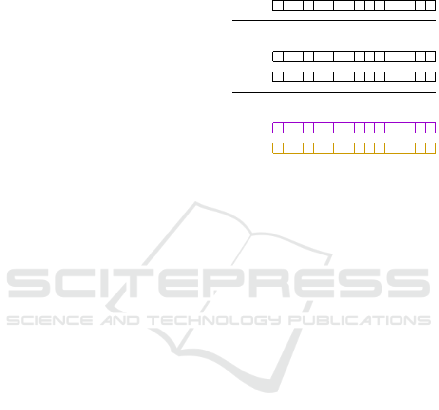
In Figure 2, you can see how to derive 32-bit vec-
tors for the “nucleotides” R and M, and how to deter-
mine if there are any N-symbols in the string. To ac-
complish this, right-shift operations by 32 and 64 bits
are utilized, combined with bitwise logical OR oper-
ations.
The original 128-bit vector, written according to
the agreed storage scheme, is referred to as v
1
. The
vector v
2
= v
1
≫ 32 contains data for C, G, and T
in the first, second, and third 32-bit blocks, respec-
tively, while the fourth block consists entirely of ze-
roes. Similarly, v
3
= v
1
≫ 64 retains only the bits for
G and T.
Next, the vector v
4
= v
1
|v
2
holds the bits corre-
sponding to M in the first 32-bit block, and the vec-
tor v
6
= v
1
|v
3
contains the bits for R in the first 32-
bit block. Furthermore, the first 32 bits of v
7
=
v
4
|(v
4
≫ 64) can be used to check for the presence
of N-symbols, indicated by the corresponding bits be-
ing zero.
Algorithms for Fast and Efficient Sequence Alignment
621

Original 128-bit block (32-bit blocks for A, C, G, T bits)
v
1
A
C G
T
Shifting the origin al blocks by 32 and 64 bits
v
2
= v
1
> > 32
C G
T
v
3
= v
1
> > 64
G
T
Logical OR operation for the above data
v
4
= v
1
| v
2
v
5
= v
4
> > 64
v
6
= v
1
| v
3
v
7
= v
4
| v
5
A | C C | G G | T
T
G | T
T
A | G C | T
G
T
A | C | G | T C | G | T G | T
T
Figure 2: Determining R and M-bits for a given 128-bit data
structure (the first blocks for v
6
and v
4
vectors). The pres-
ence of N-symbols can be found with the first 32-bit block
of v
7
vector.
3 SEED HASHING
Let us consider a general case involving a ternary
seed. This seed consists of a string of three characters:
# (representing a match), @ (representing a transition
match), and _ (representing a “don’t care” symbol), as
defined in (No
´
e and Kucherov, 2004). The length of
this string is denoted as s. We also examine a genetic
sequence that has the same length s and contains no
N-symbols. Our objective is to convert the given ge-
netic sequence into a numerical representation, often
referred to as a hash or a “signature” (Titarenko and
Titarenko, 2023).
To achieve this, we will select an element L
i
from
the genetic sequence and consider the corresponding
element S
i
from the seed. For each letter L
i
, we derive
two bits: R
i
and M
i
. Next, we will determine which
bits from R and M will be retained based on the follow-
ing rules:
• If S
i
= _, we ignore the element L
i
and thus dis-
card both the R
i
and M
i
bits.
• If S
i
= @, we keep the R
i
-bit, discard the M
i
-bit.
• If S
i
= #, we keep both the R
i
-bit and the M
i
-bit.
The simplest approach is to remove all gaps from
the R- and M-vectors and then concatenate the re-
maining bits.
A similar procedure can be applied to a single read
or the entire reference sequence, as illustrated in Fig-
ure 3. If the read has a length of r and the seed length
is s, there are (r − s + 1) possible starting positions
within the read where the entire seed can fit. As a
result, we can generate (r − s + 1) records, each for-
matted as (“signature”, position). The “signature” is a
2w-bit number (where w is the weight of the seed) and
is derived using the previously mentioned procedure.
A sequence alignment algorithm that utilises lookup
tables employs these “signatures” generated for each
read. By accessing the library of records for the ref-
erence sequence, we can identify potential alignment
positions of the read within the reference sequence.
3.1 Compacting Spaced Seeds
The outcome of applying a sequence alignment al-
gorithm remains unchanged if we shuffle all the bits
within the “signature”/hash number. By shuffling, we
mean a bijective operation, where each original index
corresponds to one unique new index, and all new in-
dices are different. Specifically, for indices i
k
where
k = 1, ...,2w, it holds that 1 ≤ i
k
≤ 2w, and for any i
k
and i
m
where k ̸= m, we have i
k
̸= i
m
.
Next, let’s explore the problem of rearranging ele-
ments of a string with gaps to create a new string with-
out gaps. We intend to use left and right shift opera-
tions, along with masking operations to select specific
bits for the new string. Assume that both masking and
shifting operations can be applied to the entire string
and have the same cost. Therefore, moving three sym-
bols to the right by five positions incurs the same cost
as moving seven symbols to the left by two positions.
As we plan to utilise SIMD instructions later, we
introduce an additional restriction: we want to fill the
leftmost gaps only. This approach helps us keep the
data aligned to specific memory boundaries.
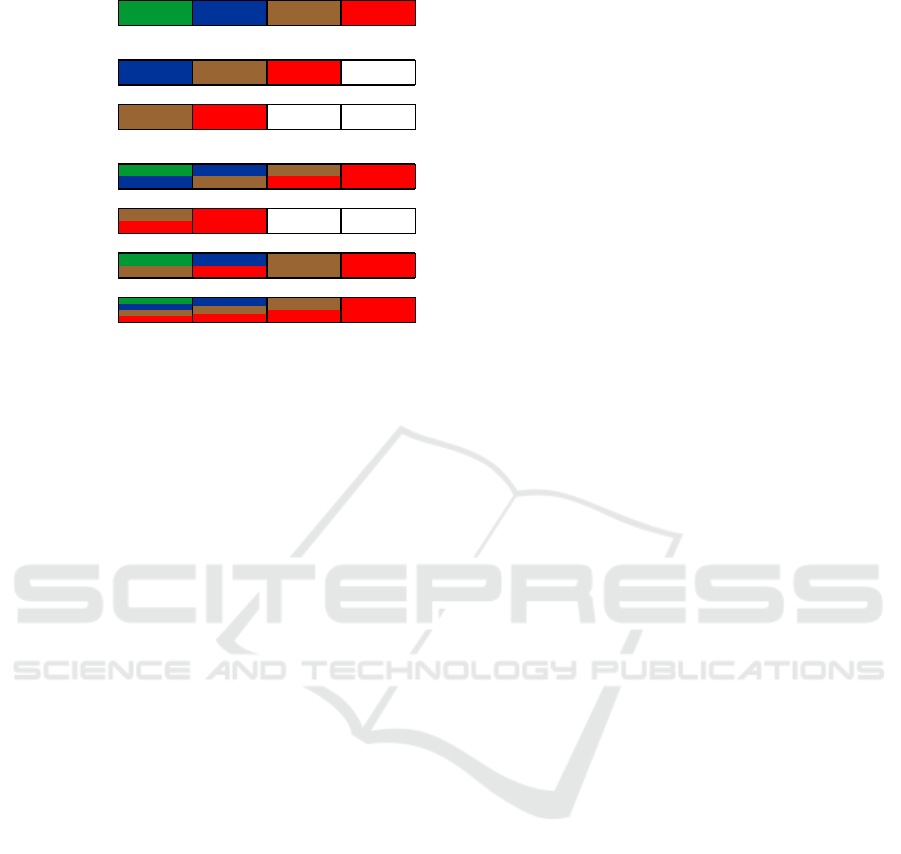
Figure 4 illustrates the procedure for compacting
a string. The blue colour and the letter L represent the
symbols that we keep in their original positions, while
the colours indicate the symbols that will be shifted.
The string has a length of 31 and a weight of 16, so
we aim to fill all gaps within the first 16 elements.
To achieve this, we divide the string into the first 16
elements on the left and the last 15 on the right.
Within the left part of the string, there are eight
gaps (0-elements), while the right part contains the
same number of non-gap elements. We can imple-
ment a simple approach to address this. First, we
identify the first position of a non-gap element in the
right chunk and the first position of a gap in the left
chunk. We then perform a shift; in this case, we shift
by 14 elements. Additionally, we can shift five other
non-gap elements simultaneously. After this initial it-
eration, only three non-gap elements remain.
We continue this process through three additional
operations. Therefore, our naive approach requires
four iterations. In some cases, the solution may be
reduced to just three iterations.
BIOINFORMATICS 2025 - 16th International Conference on Bioinformatics Models, Methods and Algorithms
622

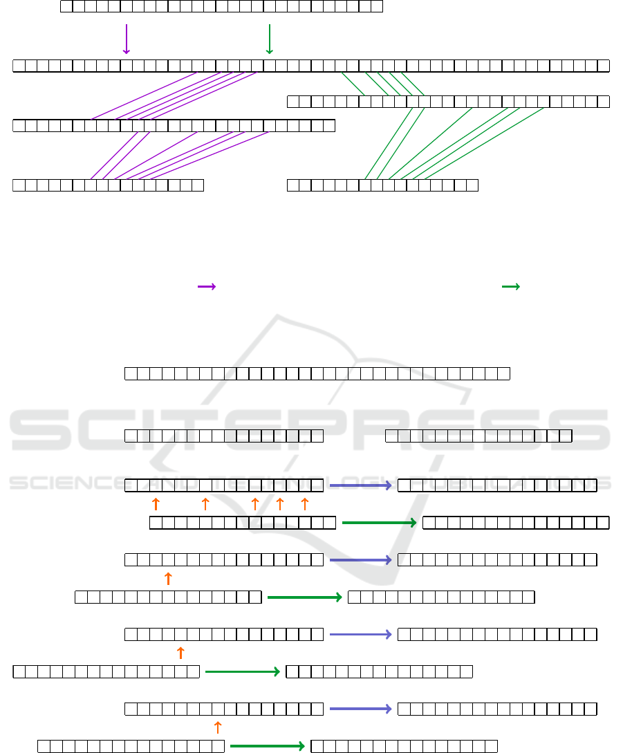
Seed
# _ _ # # _ # _ # # # # _ _ _ # _ _ # # _ # _ # # # #
A chunk of a long sequence
G
T T
C
A A
G
T
G
T
C C C
A A
C
T
C
T
G C G C
T
C
A
G
A A
C
T
G
A A T
C
T
G C
T
G G
T
G G
A
G
A A
G
Position = 246326 Position = 246338
T
C
A
C C
T
G C C
A A T A A T
C
G C
A A
C
T
G
A T T
G
T
G
A
G
A
T
C
A
C C
T
G C C
A A T A A T
C G C
A A
C
T
G
A T T
G
T
G
A
G
A
11100010101101101000001100001110 = 70c16d47 01100000101101001111011101000100 = 22ef2d06
Extracting chunks and
accounting for seed’s bits
Compacting sequences
Binarisation (A = 0, C = 1, G = 2, T = 3), forming hex “signatures”
Library of records (“signature”, position)
(
87ad5e86, 246317)
(215b57c3, 246318)
(
08e515a3, 246319)
(
425b05f9, 246320)
(
d036416c, 246 321)
(b49dd078, 246322)
(
2d06745e, 246323)
(
0b21dd17, 246324)
(
c24bb716, 246325)
(70c16d47, 246326)
(
dc909bc1, 246327)
(
b7366651, 246328)
(
6d2cd9f5, 246329)
(dbc8769c, 246330)
(
b6411d74, 246331)
(
adf387ad, 246332)
(
eb9e215b, 246333)
(ba7408e5, 246334)
(
aeec425b, 246335)
(
2b9bd036, 246336)
(
8ab5b49d, 246337)
(22ef2d06, 246338)
(
08aa0b21, 246339)
(
82b9c24b, 246340)
Figure 3: Forming a library of records for a reference sequence.
1) Original string
L L
0 0 0
L
0 0
L L
0
L
0
L
0
L L
0 0 0
L
0 0
L L
0
L
0
L L L
2) Length (total number of elements, 31) Weight (number of non-zero elements, 16)
Splitting the sequence (16 first and 15 last elements)
L L
0 0 0
L
0 0
L L
0
L
0
L
0
L L
0 0 0
L
0 0
L L
0
L
0
L L L
3) Aligning the first non-zero element of the right sequence to the first gap of the left sequence (shift by 14)
L L
0 0 0
L
0 0
L L
0
L
0
L
0
L
L
0 0 0
L
0 0
L L
0
L
0
L L L
L L L
0 0
L L
0
L L L L L L L L
0 0 0 0 0 0 0
L
0 0 0 0 0
L L
4) Aligning the first non-zero element of the right sequence to the first gap of the left sequence (shift by 20)
L L L
0 0
L L
0
L L L L L L L L
0 0 0 0 0 0 0
L
0 0 0 0 0
L L
L L L L
0
L L
0
L L L L L L L L
0 0 0 0 0 0 0 0 0 0 0 0 0
L L
5) Aligning the first non-zero element of t he right sequence to the first gap of the left sequenc e (shift by 25)
L L L L
0
L L
0
L L L L L L L L
0 0 0 0 0 0 0 0 0 0 0 0 0
L L
L L L L L L L
0
L L L L L L L L
0 0 0 0 0 0 0 0 0 0 0 0 0 0
L
6) Aligning the first non-zero element of the right sequence to the first gap of the left sequence (shift by 23)
L L L L L L L
0
L L L L L L L L
0 0 0 0 0 0 0 0 0 0 0 0 0 0
L
L L L L L L L L L L L L L L L L
0 0 0 0 0 0 0 0 0 0 0 0 0 0 0
Figure 4: A naive approach to compact a string with gaps.
3.2 Operations with Spaced Seeds
The previous analysis suggests that more effective
methods exist than the naive approach. Our objec-
tive is to examine all possible combinations using the
minimum number of iterations, ideally.
We can create two arrays of positions: one for the
gaps (0-elements) in the left chunk and another for
the non-gaps (L-elements) in the right chunk, as il-
Algorithms for Fast and Efficient Sequence Alignment
623

lustrated in Algorithm 1. We will analyze all possi-
ble shifts to ensure that at least one L-element from
the right chunk aligns with a 0-element from the left
chunk. It is important to note that other L-elements
may extend beyond the limits of the string. There
are a total of 24 shifts to consider. This results in a
matrix with dimensions of 24 × 8, where 8 represents
the number of variables (gaps for the left chunk or
L-elements for the right chunk). Our next step is to
evaluate all possible combinations of the rows in this
matrix.
Input: binary array v of length s
Output: arrays of positions for gaps, I
gap
,
and ones, I
one
w ← 0 ; /* weight */
for i = 1 to s do
if v[i] = 1 then
w ← w + 1
end
end
g ← 0 ; /* number of variables */
for i = 1 to w do
if v[i] = 0 then
g ← g + 1;
I
gap
[g] ← i;
end
end
g ← 0;
for i = w + 1 to s do
if v[i] = 1 then
g ← g + 1;
I
one
[g] ← i;
end
end
Algorithm 1: Calculating seed’s weight w, number of vari-
ables g and arrays of positions for gaps and ones.
Let’s create a new, smaller matrix that has the
same number of columns as the original matrix. Each
column corresponds to a specific gap in the left chunk
of data. A positive element in the matrix indicates
the corresponding index of the L-element in the right
chunk of the string. If there are no L-elements from
the right chunk that correspond to a given chosen gap,
the matrix element will be zero.
Our goal is to fill all gaps, ensuring that each col-
umn contains at least one positive element. Further-
more, since all L-elements in the right chunk need to
be relocated, the new matrix must include every ele-
ment from 1 to g. Ideally, we want the matrix to con-
tain only g positive elements, all of which should be
unique. However, this is a rare occurrence. Typically,
additional processing of the matrix is required. The
only operation we can perform is to set some positive
elements to zero. This action means we disregard cer-
tain L-elements that are positioned in front of gaps in
the left chunk of the string.
Suppose there are two elements, α > 0, in a ma-
trix, and one of these elements is the only positive
element in its column. Since there can only be one
occurrence of the element α in the matrix, we need
to remove one of them. If we eliminate the element
that is the only positive in its column, that column will
contain all zero elements, resulting in no L-elements
corresponding to that gap.
Therefore, if a column contains one positive ele-
ment, α, no other elements in the matrix can equal α.
Hence, we can safely remove the remaining instance
of α. This procedure can be applied iteratively across
the matrix because by removing certain elements, we
might reveal other columns that contain only one pos-
itive element. This process is outlined in Algorithm
2.
It is possible for this procedure to leave us with
columns containing only zero elements, indicating
that the resulting matrix cannot provide a solution.
We can implement the matrix-clearing procedure us-
ing binary vectors. For each row of the matrix, we
maintain two binary vectors: one to indicate whether
a cell is occupied or vacant, and another to store the
values of the positive elements. Logical OR opera-
tions will help us identify whether a column contains
zero, one, or multiple positive elements. The same
method applies when checking for the presence of a
specific L-element in the matrix.
After the clearing procedure, there may be
columns containing several positive elements. In this
case, we select one of these columns (ideally, the
one with the fewest positive elements), consider all
its positive elements, and assume that only one is
present.
Suppose there are N
r
rows in the original matrix,
and we form a new matrix with N
c
selected rows. This
means we need to consider C
N
c
N
r
combinations. By def-
inition, the number of m-combinations in a set of n
elements is given by the formula:
C
m
n
≡
n!
m!(n − m)!
. (1)
Note that different notations may be used in the liter-
ature, where m! ≡ m·(m−1)·· · 2 ·1. For the example
above, we need to consider C
3
24
= 2024 cases. We
should avoid checking combinations of certain rows.
For instance, if rows 1, 5, and 20 contain one, two,
and three positive elements, respectively, their total of
positive elements is 1 + 2 + 3 = 6, which is less than
8 — the total number of variables. Therefore, we can
sort the rows of the matrix so that the total number of
BIOINFORMATICS 2025 - 16th International Conference on Bioinformatics Models, Methods and Algorithms
624

Input: submatrix S (number of rows m and
columns g)
while b = true do
b ← true;
for i = 1 to g do
k ← 0;
for j = 1 to m do
if S[ j,i] > 0 then
α ← S[ j,i];
k ← k + 1;
end
end
if k = 1 then
for p = 1 to m do
for q = 1 to g do
if S[p,q] = α and q ̸= i
then
S[p,q] ← 0;
b ← false;
end
end
end
end
end
end
Algorithm 2: Elimination of matrix elements for columns
containing one positive element.
positive elements does not decrease with the row in-
dex.
We can use an iterative process to select N
c
dif-
ferent rows. For simplicity, we assume that I
k
> I
k−1
since the order of the rows is not important. The first
row will be assigned the index I
1
∈ [1,N
r
− N
c
+ 1].
The second row will have the index I
2
∈ [I
1
+ 1,N
r
−
N
c
+ 2], and in general, I
k
∈ [I
k−1
+ 1,N
r
− N
c
+ k].
Once we have chosen the first k indices, we can use
the binary vectors mentioned above to compute how
many columns still contain only 0-elements and how
many distinct L-elements are in the chosen rows. We
can skip further steps if the remaining number of
columns or L-elements exceeds the total number of
elements for the remaining (N
c
− k) rows, or simply
(N
c
− k) · Q, where Q is the number of positive ele-
ments in the (I
k
+ 1)-th row.
3.3 SIMD Operations
We will discuss the 128-bit representation of genetic
sequences.
Consider a genetic sequence of length s and a bi-
nary seed of the same length with weight w. Data
is organized into 128-bit blocks, each containing in-
formation about 32 symbols. The first 128-bit block
holds the first 32 symbols of the sequence. If s is not
a multiple of 32, the last block may contain additional
symbols beyond the sequence.
To determine the number of 128-bit blocks re-
quired to store the sequence, we use the formula
n
s
= ⌈s/32⌉, where ⌈x⌉ represents the smallest inte-
ger not less than x.
In this study, we will concentrate on specific
SIMD operations, including logical operations, mask-
ing, and bit shifting. While SIMD can also perform
operations like shuffling and interleaving blocks, we
will not include these in our analysis.
Our objective is to compact the data by filling the
initial gaps in the sequence, guided by a seed. For a
given weight w of the seed, we count the number g
of gaps within the first w symbols. This results in g
1-elements positioned in the seed’s last (s − w) ele-
ments. We aim to relocate these g elements within the
sequence, allowing for some flexibility even without
shuffling.
For instance, if we have three 128-bit blocks,
we can reorder (or access) them in six different
ways: (1,2,3), (1, 3,2), (2,1, 3), (2,3,1), (3,1, 2),
and (3,2, 1). This results in n
s
! options for n
s
blocks.
Next, we calculate the total number N of problems
to be solved. We define n
w
≡ ⌊w/32⌋ (where ⌊x⌋ is the
largest integer not greater than x) and r
w
= w − 32n
w
,
the remainder. If r
w
= 0, we need to count the to-
tal number of combinations C
n
w
n
s
; therefore, N = C
n
w
n
s
.
The order of the chosen n
w
elements and the remain-
ing (n
s
− n
w
) elements does not matter.
For example, if n
s
= 4 and n
w
= 2, we can form 24
sets of four numbers: (1, 2,3,4), (1,2,4,3), and so on.
However, the order of elements in the first two and last
two positions is not important, since combinations
like (1,2,3,4), (2, 1, 3,4), (1,2,4, 3), and (2,1,4, 3)
are considered equivalent. Although the packed se-
quences formed using different 128-bit blocks are dis-
tinct, the total number of operations remains the same.
Therefore, they are equal in terms of performance.
If r
w
̸= 0, we calculate the total number of vari-
ants differently. We need to choose a 128-bit structure
where these r
w
elements are. There are n
s
cases. For
the remaining (n
s
− 1), we count the number of n
w
-
combinations. So, N = n
s
C
n
w
n
s
−1
. We may see that the
second case (r
w
̸= 0) generates (n
s
− n
w
) times more
problems compared to the first case (r
w
= 0).
Each of the N problems has varying gaps g, but the
total weight w is constant. We fix a number of rows in
a submatrix and process all problems. If any problem
finds a solution, we stop; otherwise, we increase the
number of rows.
In Figure 2, we see how R, M, and A|C|G|T 32-bit
blocks are formed within a 128-bit block. A ternary
Algorithms for Fast and Efficient Sequence Alignment
625

seed generates two binary seeds: the #-seed requires
both R and M bits, while the @-seed uses only R bits.
The final “signature” number is created by concate-
nating the results from both seeds. Alternatively, full
32-bit blocks can be combined first, followed by in-
complete blocks.
4 CONCLUSION
We have developed algorithms to calculate hash val-
ues for spaced seeds and genetic sequences. These al-
gorithms are designed to leverage SIMD instructions,
enabling the formation of numbers using as few oper-
ations as possible. We started with a straightforward
method for compacting strings with gaps, which in-
volves shifting and masking operations.
Public codes to generate these functions are
at https://github.com/vtman/comBiTeS. Examples of
codes to pre-align reads using these functions are at
https://github.com/vtman/perlotSeeds, and the results
of their application to real data are at (Titarenko and
Titarenko, 2024).
The next step is to profile our developed code
against existing alignment solutions. Additionally, we
will explore advanced shuffling techniques and data
interleaving operations for further investigation.
REFERENCES
Altschul, S. F., Gish, W., Miller, W., Myers, E. W., and
Lipman, D. J. (1990). Basic local alignment search
tool. Journal of Molecular Biology, 215(3):403–410.
Baichoo, S. and Ouzounis, C. A. (2017). Computational
complexity of algorithms for sequence comparison,
short-read assembly and genome alignment. Biosys-
tems, 156-157:72–85.
Brejov
´
a, B., Brown, D. G., and Vina
ˇ
r, T. (2005). Vector
seeds: an extension to spaced seeds. Journal of Com-
puter and System Sciences, 70(3):364–380.
Buhler, J. (2001). Efficient large-scale sequence compar-
ison by locality-sensitive hashing. Bioinformatics,
17(5):419–428.
Delcher, A. L., Kasif, S., Fleischmann, R. D., Peterson,
J., White, O., and Salzberg, S. L. (1999). Align-
ment of whole genomes. Nucleic Acids Research,
27(11):2369–2376.
Feng, D., Johnson, M., and Doolittle, R. (1985). Align-
ing amino acid sequences: Comparison of com-
monly used methods. Journal of Molecular Evolution,
21(2):112–125.
Firtina, C., Park, J., Alser, M., Kim, J. S., Cali, D.,
Shahroodi, T., Ghiasi, N., Singh, G., Kanellopoulos,
K., Alkan, C., and Mutlu, O. (2023). BLEND: a
fast, memory-efficient and accurate mechanism to find
fuzzy seed matches in genome analysis. NAR Ge-
nomics and Bioinformatics, 5(1):lqad004.
Girotto, S., Comin, M., and Pizzi, C. (2018). Efficient com-
putation of spaced seed hashing with block indexing.
BMC Bioinformatics, 19(15):441.
Gotoh, O. (1982). An improved algorithm for matching
biological sequences. Journal of Molecular Biology,
162(3):705–708.
Graur, D. and Li, W.-H. (2000). Fundamentals of Molecular
Evolution. Sinauer, Sunderland, MA, 2 edition.
Hamming, R. W. (1950). Error detecting and error cor-
recting codes. The Bell System Technical Journal,
29(2):147–160.
Intel (2023). Intel intrinsics guide. www.intel.com/content/
www/us/en/docs/intrinsics-guide/index.html.
Li, H. and Durbin, R. (2009). Fast and accurate short read
alignment with Burrows–Wheeler transform. Bioin-
formatics, 25(14):1754–1760.
Ma, B., Tromp, J., and Li, M. (2002). PatternHunter: faster
and more sensitive homology search. Bioinformatics,
18(3):440–445.
Mak, D., Gelfand, Y., and Benson, G. (2006). Indel seeds
for homology search. Bioinformatics, 22(14):e341–
e349.
Myers, E. W. and Miller, W. (1988). Optimal alignments in
linear space. Bioinformatics, 4(1):11–17.
Needleman, S. B. and Wunsch, C. D. (1970). A gen-
eral method applicable to the search for similarities
in the amino acid sequence of two proteins. Journal
of Molecular Biology, 48(3):443–453.
No
´
e, L. and Kucherov, G. (2004). Improved hit criteria for
DNA local alignment. BMC Bioinformatics, 5(1):149.
Pearson, W. R. and Lipman, D. J. (1988). Improved tools
for biological sequence comparison. Proc. Natl. Acad.
Sci. USA, 85(8):2444–2448.
Sessions, S. (2013). Genome size. In Maloy, S. and Hughes,
K., editors, Brenner’s Encyclopedia of Genetics (Sec-
ond Edition), pages 301–305. Academic Press, San
Diego, 2 edition.
Smith, T. F. and Waterman, M. S. (1981). Identification of
common molecular subsequences. Journal of Molec-
ular Biology, 147(1):195–197.
Titarenko, V. and Titarenko, S. (2023). PerFSeeB: Design-
ing long high-weight single spaced seeds for full sen-
sitivity alignment with a given number of mismatches.
BMC Bioinformatics, 24:396.
Titarenko, V. and Titarenko, S. (2024). Examples of se-
quence alignment with contiguous, binary and ternary
seeds. 10.5281/zenodo.10645042.
Waterman, M., Smith, T., and Beyer, W. (1976). Some bi-
ological sequence metrics. Advances in Mathematics,
20(3):367–387.
Wilbur, W. J. and Lipman, D. J. (1983). Rapid similarity
searches of nucleic acid and protein data banks. Proc.
Natl. Acad. Sci. USA, 80(3):726–730.
Xu, J., Brown, D., Li, M., and Ma, B. (2006). Optimizing
multiple spaced seeds for homology search. Journal
of Computational Biology, 13(7):1355–1368.
BIOINFORMATICS 2025 - 16th International Conference on Bioinformatics Models, Methods and Algorithms
626