Agent-Based Computational Geometry

Akbarbek Rakhmatullaev

, Shahruz Mannan

, Anirudh Potturi

and Munehiro Fukuda

Division of Computing and Software Systems, University of Washington Bothell, U.S.A.

{akbarbek, mannans1, anii, mfukuda}@uw.edu

Keywords:

Agent-Based Modeling, Data Streaming, Message Passing, Computational Geometry, Cluster Computing.

Abstract:

Cluster computing can increase CPU and spatial scalability of computational geometry. While data-streaming

tools such as Apache Sedona (we simply call Sedona) lines up built-in GIS parallelization features, they require

a shift to their programming paradigm and thus a steep learning curve. In contrast, agent-based modeling is

frequently used in computational geometry as agent propagation and ﬂocking simulate spatial problems. We

aim to identify if and in which GIS applications agent-based approach demonstrates its efﬁcient paralleliz-

ability. This paper compares MASS, Sedona, and MPI, each representing agent-based, data-streaming, and

baseline message-passing approach to parallelizing four GIS programs. Our analysis ﬁnds that MASS demon-

strates its simple programmability and yields competitive parallel performance.

1 INTRODUCTION

Cluster computing gives more CPU and spatial scal-

ability to GIS parallelization. Actual implementa-

tions include SpatialHadoop (Eldawy and Mokbel,

2015) and Apache Sedona (Yu et al., 2019), many

of which maintain spatial data in distributed storage

such as Hadoop; process the data in batches with data-

streaming tools including Spark; and respond to an-

ticipated GIS queries through a front-end interface,

(e.g., HIVE). However, the nature of data streaming is

their major challenge: besides their unique program-

ming paradigm, they need to ﬂatten, stream, shufﬂe,

and sort spatial data structures at every computational

stage, all resulting in substantial overheads.

In contrast to data streaming, we consider an

agent-based approach that maintains GIS data as a

multi-dimensional or graph structure over distributed

memory; dispatches agents as active data analyzers;

and solves spatial queries through collective group

behaviors among the agents, (e.g., agent propaga-

tion, swarming, and collision) over the data structure.

Our research motivation is to verify the efﬁciency of

the agent-based approach to computational geometry,

as compared to the conventional data-streaming ap-

proach. We believe that this research makes two con-

tributions to parallel computing in computational ge-

https://orcid.org/0009-0005-3376-0684

https://orcid.org/0009-0009-4628-5316

https://orcid.org/0000-0002-9270-9628

https://orcid.org/0000-0001-7285-2569

ometry: (1) a development of geometric benchmark

programs demonstrates that agent code is intuitive

and smoothly ﬁts the idea of spatial cognition (Freksa

et al., 2019) and (2) agent-based approach is competi-

tive to data streaming in some geometric applications

that take advantage of agent ﬂocking in a 2D space

or agent traversing over a tree, both performed over a

cluster system.

The rest of the paper is organized as follows: Sec-

tion 2 explores related work; Section 3 explains the

MASS (Multi-Agent Spatial Simulation) library; Sec-

tion 4 parallelizes GIS programs in agent-based, data-

streaming, and message passing approach; Section

5 compares their parallelization; and Section 6 con-

cludes our work.

2 RELATED WORK

Below we explore related work in data-streaming and

agent-based approach to GIS parallelization.

2.1 Challenges in Parallelizing

Geometric Problems

GEOS and CGAL are well-known C++ libraries

that implement computational-geometry algorithms

as built-in functions. Their native executions with

multithreading are the fastest but limited to a sin-

gle machine. The problem is that they are not so

worthwhile being parallelized over a cluster system

Rakhmatullaev, A., Mannan, S., Potturi, A. and Fukuda, M.

Agent-Based Computational Geometry.

DOI: 10.5220/0013240800003890

Paper published under CC license (CC BY-NC-ND 4.0)

In Proceedings of the 17th International Conference on Agents and Artiﬁcial Intelligence (ICAART 2025) - Volume 1, pages 515-522

ISBN: 978-989-758-737-5; ISSN: 2184-433X

515

that only incurs more communication overheads than

their single-machine execution. JavaGeom and JTS

are Java versions of computational-geometry libraries

that intend to ease geometric computation. Due

to their interpretive execution, they do not outper-

form C++ libraries but show competitive processing

throughput if a dataset size is maximized to the under-

lying memory space. In general, sequential or multi-

threaded execution runs fastest but its spatial scalabil-

ity is restricted to a single machine’s memory space.

2.2 Data Streaming to CPU Cores

As data streaming keeps receiving great popularity

in big data, it is quite natural and convenient to in-

tegrate data-streaming tools into a GIS system for

scalable spatial analysis. A typical architecture mod-

iﬁes a Lambda service layer tool, (e.g., HIVE) for

a real-time GIS query interface, uses data-streaming

tools such as MapReduce and Spark for preparing an-

ticipated query responses, and maintains entire spa-

tial datasets in a backend database including Post-

GreSQL. For instance, SpatialHadoop interfaces to

users through Pigeon, a SQL-like language, which re-

lays their queries to MapReduce for geometric com-

putation (Eldawy and Mokbel, 2015). Sedona re-

ceives a spatial query through its Spatial SQL API

that chooses the corresponding geometric algorithm,

(e.g., range search, distance joining, and KNN) in the

Spatial Query Processing Layer. The selected algo-

rithm is then carried out though operations on Spatial

RDDs, an extension of Spark RDDs (Resilient Dis-

tributed Datasets) (Yu et al., 2019). For graph com-

puting, GraphX extends Spark RDDs to edge and ver-

tex RDDs, and supports Pregel’s graph API (Spark

GraphX, 2018)

In general, data streaming must disassemble GIS

ﬁles into texts and repeat series of data shufﬂe and

sort, as computational geometry is optimized in the

divide-and-conquer paradigm, which may slow down

geometric analysis.

2.3 Migrating Agents over GIS Data

We consider applying agent-based modeling (ABM)

to computational geometry. This idea is found in the

following three ABM libraries:

NetLogo approximates a 2D radical propaga-

tion of agents by repetitively cloning agents to von-

Neumann and Moore neighborhoods in an alterna-

tive fashion (Wilensky, 2013). Using this agent

propagation from each data point, NetLogo com-

poses a Voronoi diagram as collision lines between

agents. Repast Simphony (North et al., 2007) pop-

ulates agents on all the four boundary lines of a 2D

space and march them toward the center of the space.

This is a simulation of wrapping data points with an

elastic band, which forms the convex hull. GeoMA-

SON allows agents to migrate on geospatial compo-

nents such as line segments and polygons (Sullivan

et al., 2010). It also computes the shortest path on

a network of line segments and their intersections as

built-in functions.

Their biggest challenge is single-machine execu-

tion. Because of their difﬁculty in being extended to

cluster computing, they cannot support spatial scala-

bility nor parallelize ﬁle I/Os. This is our motivation

to apply MASS, a parallel ABM library to more ad-

vanced spatial problems.

3 COMPUTATIONAL MODEL

This section summarizes the MASS library’s compu-

tational model and introduces its extension to graph

and geometric computing.

3.1 MASS Library

MASS distinguishes two classes: Places and Agents.

The former is a multi-dimensional array distributed

over a cluster system. Each array element is called

“place” and is identiﬁed with a platform-independent

logical index. The latter is a collection of mobile ob-

jects, each called “agent”, capable of moving to a dif-

ferent place.

Listing 1 shows MASS code. The main() function

serves as a simulation scenario. MASS.init() launches

a multithreaded, TCP-communicating process at each

machine (line 3). Lines 4-6 create an x × y 2D Places

and populate Agents. Places has two parallel func-

tions: callAll() to invoke a given function, (e.g., up-

date func on line 7) at each place in parallel and ex-

changeAll() to have each place communicate with all

its neighbors, (e.g., diffuse func in line 8). Agents

has two parallel functions, too. One is callAll() that

schedules agent behavior with spawn(), kill(), and mi-

grate() (line 9). The other is manageAll() that com-

mits their scheduled behaviors (line 10). Finally,

MASS.ﬁnish() closes all MASS processes (line 11).

Listing 1: MASS abstract code.

1 public class MassAppl {

2 public static void main(String args[]) {

3 MASS.init( );

4 Places map = new Places("Map", args, x, y);

5 Agents crawlers

6 = new Agents("Crawlers", args, map);

7 map.callAll(update func, args);

8 map.exchangeAll(diffuse func);

ICAART 2025 - 17th International Conference on Agents and Artiﬁcial Intelligence

516

9 crawlers.callAll(walk func, args);

10 crawlers.manageAll( );

11 MASS.ﬁnish( );

12 } }

3.2 Agent Descriptions in Graph and

Geometric Problems

To facilitate GIS computation, MASS improved the

following ﬁve features: (1) GraphPlaces: a Places

sub-class that instantiates place objects as graph ver-

tices whose emanating edges are deﬁned in the neigh-

bors list as one of their data members; (2) Binary-

TreePlaces: a special form of GraphPlaces to distin-

guish only left and right child vertices, which eases

KD-tree operations in range search; (3) SpacePlaces:

a 2D contiguous space, using QuadTreePlaces that re-

duces the number of place objects in memory as well

as mitigates unnecessary agent migration. The closet

pair of points, convex hull, and Voronoi problems use

this class; (4) SmartAgents: an Agents sub-class that

automates agent propagation over a GraphPlaces, a

BinaryTreePlaces, and a SpacePlaces instance, each

used in the breadth-ﬁrst search, the range search, and

all the 2D geometric problems; and (5) GUI: an in-

terface to the JShell interpreter and the Cytoscape vi-

sualizer. These features make MASS competitive to

data-streaming tools in programmability and in exe-

cution performance.

4 PARALLELIZED

ALGORITHMS

Our expectation is two-fold: agents could identify

a given geometric shape faster if their ﬂocking con-

verges to a small space, and they could quickly re-

spond to geometric queries if they use the same data

structure that stays in memory. From these view-

points, we have chosen the following four geomet-

ric problems for our comparative work: (1) convex

hull, (2) Euclidean shortest path, (3) largest empty cir-

cle, and (4) range search. Below we parallelize these

programs using MASS, Sedona, and MPI, each rep-

resenting agent-based, data-streaming, and conven-

tional message-passing approach.

4.1 Convex Hull (CVH)

4.1.1 Agent-Based Approach

MASS has agents swarm inward from the outer edges

of a given space until they encounter any data points,

which simulates wrapping all points with a rubber

band. The algorithm is coded in Listing 2. It popu-

lates agents on the four boundary edges of a size×size

space (lines 4-5), marches them until they hit a point

(lines 10-13), excludes unvisited points (lines 15), and

retrieves all data points on the ﬁnal convex hull (lines

16-17). As some data points may be mistakenly de-

tected as vertices of the convex hull, they must be re-

moved by Andrew’s monotone chain algorithm.

Listing 2: Convex hull using MASS.

1 public class CVH {

2 public static void main(String args[]) {

3 Places places = new Places("AreaGrid", size , size)

;

4 Agents agents = new Agents("RubberBandAgent",

5 places, size

4);

6 agents.callAll(RubberBandAgent.

7 SET START POSITION);

8 agents.manageAll();

9 // March agents toward the center like a rubber

band

10 while (agents.nAgents() > 0) {

11 agents.callAll(RubberBandAgent.MOVE);

12 agents.manageAll();

13 }

14 // Remove inner points and collect those on the hull

15 places.callAll(AreaGrid.CLEAR INNER PLACES)

;

16 Object[] oResults

17 = places.callAll(AreaGrid.GET PTS, null);

18 } }

4.1.2 Data-Streaming Approach

Sedona takes a divide-and-conquer approach that

spreads out all data points to partitions, creates a per-

partition convex hull, and aggregates together all the

partial hulls into the ﬁnal convex hull. In order to

achieve this, we ﬁrst create a spatialRDD and then

partition it using Sedona’s EQUALGRID type, as it

shows the best execution performance among other

grid types. Next, each partition creates a list of its

points, from which we create a multi-point object of

Sedona’s Geometry class. Then, we call Sedona’s

built-in convexHull() function on this multi-point ob-

ject to create a per-partition convex hull, where each

convex hull is stored as a singleton collection. Fi-

nally, we aggregate all partial hulls into a table and

apply Sedona’s SQL functions ST ConvexHull and

ST Union Aggr to produce the ﬁnal hull, a single-row

dataset representing the complete convex hull.

4.1.3 Message-Passing Approach

MPI needs to sort input data, based on the x coordi-

nate. Then, it partitions the data and distributes the

subsets to each rank. Thereafter, the monotone chain

algorithm is used to compute the convex-hull points at

each rank. The algorithm constructs the upper and the

Agent-Based Computational Geometry

517

lower hull separately, followed by combining them

into a complete hull.

After creating a partial hull on every rank,

MPI Send() and MPI Recv() are called between two

neighboring ranks to merge their partial hulls into a

larger hull. A typical O(N) merging algorithm is used

to ﬁnd the upper/lower tangent lines connecting two

hulls and to remove the points between them. This

merging step is repeated until all hulls are combined

into the ﬁnal convex hull at rank 0.

4.2 Euclidean Shortest Path (ESP)

4.2.1 Agent-Based Approach

Starting from a source, agents repeat bouncing obsta-

cles or terminating themselves if others have visited

the current grid, which eventually carries the fastest

agent to a given destination. Listing 3 initializes a

2D space with obstacles (line 4), positions a Rover

agent at a source point (lines 5-8), and then falls into

an agent propagation loop (lines 9-19) until an agent

reached the goal (line 9). Each iteration clones agents

if they are the ﬁrst visitor on the current grid that is

not yet the destination (lines 13-16); moves all the

cloned agents to non-blocking neighbors (lines 17-

18); marks each grid with the ﬁrst agent’s footprint

(line 10); and kills all slower agents (lines 11-12).

Listing 3: Euclidean shortest path using MASS.

1 public class ESP {

2 public static void main(String args[]) {

3 Places places = new Places("Cell", sizeX, sizeY);

4 places.callAll(Cell.init , dataset);

5 Agents agents = new Agents("Rover", places, 1);

6 agents.callAll(Rover.starting point,

7 (new int[]{starting x, starting y}));

8 agents.manageAll();

9 while (!foundTarget && agents.nAgents() > 0) {

10 places.callAll(Cell.update );

11 agents.callAll(Rover.update termination);

12 agents.manageAll();

13 Object target = agents.callAll(Rover.clone,

14 new Object[agents.nAgents()]);

15 agents.manageAll();

16 if ( target ) break;

17 agents.callAll(Rover.migrate all);

18 agents.manageAll()

19 } } }

4.2.2 Data-Streaming Approach

Sedona ﬁrst includes the starting and ending points as

well as all obstacle corner points in a dataset, from

which we generate a visibility graph by forming a

Cartesian product of all points to get potential edges.

Each edge is then checked to see if it intersects any

obstacles; if not, it is considered visible between the

points and added to a list for later distance calcula-

tions. With all visible vertex combinations identiﬁed,

we apply Dijkstra’s algorithm to compute the shortest

path from the start to the endpoint.

4.2.3 Message-Passing Approach

MPI constructs a visibility graph and applies Dijk-

stra’s algorithm on it as Sedona does. Input points are

partitioned to all MPI ranks where a per-rank visibil-

ity graph is created from the subset. The simplest but

greedy approach compares every pair of points from

each subset for checking if it is a visibility edge. Once

a per-rank visibility graph is constructed, the informa-

tion is saved as a Hash-Map at each rank, where the

key is a vertex, and the value is a list of the vertices

which can create a visibility edge with this speciﬁc

vertex. Thereafter, all the partial visibility graphs are

sent back to rank 0 and combined into a complete vis-

ibility graph of all the data points. Lastly, Dijkstra’s

algorithm is used for ﬁnding the shortest path.

4.3 Largest Empty Circle (LEC)

Sedona, MASS, and MPI all take the same LEC

algorithm - convex hull and Voronoi diagram con-

structions followed by computing the center of LEC

from all Voronoi vertices and intersections between

the convex hull and the Voronoi diagram. All their

parallelization strategies also take data decomposi-

tion where each RDD partition in Sedona, each place

in MASS, and each rank in MPI reports its poten-

tial point of LEC to main(). This is because, if we

use agent propagation in MASS, the agents diverge

their population from each Voronoi vertex, thus waste

memory space, and do not perform faster.

4.3.1 Agent-Based Approach

MASS ﬁrst uses Fortune’s sweep-line algorithm to

create a Voronoi diagram sequentially from input data

points that are located within a space of w width and

h height (line 5). It then distributes the Voronoi ver-

tices and edges into nP partitions (lines 7-13). From

them, MASS creates Places (line 14), each of which

takes a different partition (line 15), computes the in-

tersections between Convex Hull edges and Voronoi

edges in the partition (line 16), and identiﬁes a po-

tential LEC center (line 18). Finally, main() collects

potential circles from all the Places and ﬁnds the ﬁnal

LEC (lines 20-23).

Listing 4: Agent-based largest empty circle.

1 public class LEC {

2 public static void main(String args[]) {

ICAART 2025 - 17th International Conference on Agents and Artiﬁcial Intelligence

518

3 Point2D[] points = dataPoints();

4 // Create Voronoi Diagram

5 Voronoi diagram = new Voronoi (w, h, points);

6 // Partition vertices

7 int vSize = diagram.vertices.length;

8 int[][] v = partitionData(diagram, vSize, nP);

9 // Partition Edges

10 int eSize = diagram.edges.length;

11 int[][] e = partitionData(diagram, eSize, nP);

12 // Create subsets

13 Object[] partitions = createPartitions(v, e, nP);

14 Places places = new Places("Partitions", nP);

15 places.callAll(Parititions.Init, partitions);

16 places.callAll(Parititions.Intersections);

17 // Compute Largest Empty Circle

18 places.callAll(Partitions.LEC, points);

19 // Return all Largest Empty Circles

20 Object[] results

21 = places.callAll(Partitions.Collect);

22 // Get The largest empty circle from all the circles

23 max(results);

24 } }

4.3.2 Data-Streaming Approach

Sedona ﬁrst constructs a convex hull, using the al-

gorithm described in Section 4.1.2. It then gener-

ates a Voronoi diagram from these points, using its

built-in VoronoiDiagramBuilder class. Thereafter,

Sedona clips the diagram along the convex hull edges

to obtain Voronoi polygons. These polygons, com-

bined with the convex hull, help identify candidate

points. The candidate points are then converted to

spatial RDD which gets partitioned, using Sedona’s

EQUALGRID. A nearest neighbor search is applied

to them within each partition to determine the center

and radius of the largest empty circle. Finally, Se-

dona combines all the centers and radiuses from all

partitions to ﬁnd the one with the largest radius.

4.3.3 Message-Passing Approach

Rank 0 sequentially creates a Voronoi diagram from

input points, using the Fortune’s sweep-line algo-

rithm. It then creates the convex hull as described

in Section 4.1.3. Next, the Voronoi vertices, Voronoi

edges, and the convex hull points are split into parti-

tions and distributed to all MPI ranks. They compute

the intersection points between the subsets of Voronoi

Edges and the Convex Hull edges in their partition.

All the ranks iteratively examine their Voronoi ver-

tices and the intersection points to calculate the radius

to their closest original data point. Their local LECs

are collected at rank 0 that ﬁnds the largest one.

4.4 Range Search (RGS)

4.4.1 Agent-Based Approach

Listing 5 outlines agent propagation down over a KD

tree from its root in search for all tree nodes in a given

range. First, MASS creates a KD tree from Graph-

Places (lines 3-4), which is the slowest part of the

code as the tree is recursively constructed from main()

(line 5). Thereafter, the initial agent starts a KD tree

search from its root (line 6) and repeats propagating

its copies along the left/right tree branches (line 7-

10). Upon every propagation down to the next tree

level, agents report back to main() if they encounter

tree nodes within a queried range (lines 8-9). Lines 6-

10 can be repetitively used for responding to different

queries. The MASS implementation’s strength is a

global KD tree construction over distributed memory.

Listing 5: Agent-based range search.

1 public class RGS {

2 public static void main(String args[]) {

3 ArrayList<Point2D> points = getPoints(inputFile);

4 GraphPlaces kdTree = new GraphPlaces("KDTree")

;

5 constructTree(kdTree, points);

6 Agents rovers = new Agents("Rover", kdTree, 1);

7 while( rovers.nAgents() > 0 ) { // tree traverse

8 Object results[] = rovers.callAll(Rover.search);

9 Collections.addAll(results); // range identiﬁed

10 rovers.manageAll();

11 } } }

4.4.2 Data-Streaming Approach

Sedona uses SpatialRangeQuery, a built-in function.

It requires only a few parameters to operate: a spatial-

RDD with data points, an Envelope deﬁning the query

boundaries, a spatial predicate, and a boolean to spec-

ify index usage. This conﬁguration enables Sedona to

identify all points within the Envelope in spatialRDD.

Before processing a query, the spatialRDD is parti-

tioned using GridType.EQUALGRID, and results are

subsequently collected.

4.4.3 Message-Passing Approach

First, data points are read from a CSV input ﬁle,

equally partitioned, and distributed to all MPI ranks.

Each rank constructs its local KD tree by recursively

selecting dimension X or Y in turn, sorting the local

points in terms of the selected dimension, splitting the

smaller and the larger half in the left and right sub-

trees. Upon a tree completion, a query about ﬁnding

points in a given range is passed to all the ranks, each

traversing its own local KD tree. Once all the ranks

have completed querying their trees, MPI Gather() is

called to collect into rank 0 all the points that are

found in a speciﬁed range.

4.5 Programmability

Having coded the four benchmark programs with the

three libraries, we summarized their programmabil-

Agent-Based Computational Geometry

519

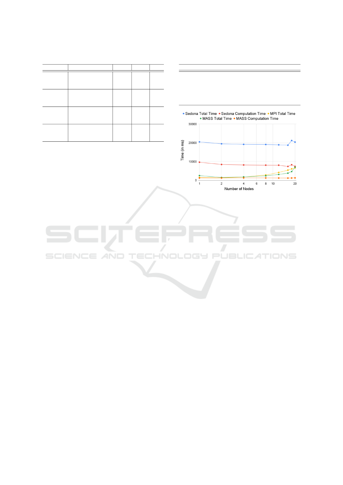
Table 1: Programmability comparison.

Benchmark Metrics Sedona MASS MPI

CVH LoC 113 710 316

Boilerplate % 43 3.8 8.8

Cyclomatic complexity 4.4 3.4 4.2

ESP LoC 191 692 523

Boilerplate % 31 5.1 4.7

Cyclomatic complexity 3.8 4.1 3.1

LEC LoC 210 767 612

Boilerplate % 41 2.5 5.2

Cyclomatic complexity 4.1 3.1 3.5

RGS LoC 120 368 233

Boilerplate % 47 4.1 8.5

Cyclomatic complexity 4.0 2.6 3.1

ity in # lines of code (LoC), boilerplate (i.e., paral-

lel code) percentage, and Cyclomatic complexity, as

shown in Table 1. In general, as Sedona lines up

built-in GIS functions, all its benchmark LoCs are the

smallest. However, this code compactness results in

increasing Sedona’s boilerplate percentage even with

a few additional statements that prepare distributed

datasets. Since the MPI benchmarks are manual ver-

sions of divide-and-conquer algorithms, their LoC is

three to ﬁve times larger than Sedona’s. However,

MPI’s boilerplate percentage and Cyclomatic com-

plexity are smaller than Sedona. This is because MPI

directly accesses each data item while Sedona repet-

itively prepares different datasets, each using lambda

expressions that handle a list of data items. In con-

trast, MASS programs end up in the largest LoC

while demonstrating the smallest boilerplate percent-

age and Cyclomatic complexity, both indicating less

semantically gapped and less branching code. Al-

though MASS facilitates intuitive agent-based coding

and parallelization, its current GIS supports such as

Graph/Tree/SpacePlaces and SmartAgents still need

to automate and to integrate more GIS features into

MASS agents.

5 EVALUATION

We conducted benchmark measurements on our own

research cluster system at University of Washington

Bothell. The system consists of 20 computing nodes,

all that are 64-bit Linux servers, each with 4 CPU

cores (@2.20-3.10GHz) and 16GB memory. Our

evaluations utilized a diverse range of GIS datasets,

as summarized in Table 2.

5.1 Convex Hull (CVH)

Figures 1 and 2 compare parallel performance of Se-

dona, MASS, and MPI when running CVH with the

Table 2: Datasets used for evaluation.

Datasets Size (points) Benchmark Programs

National USFS ﬁre occurrence 581,541 RGS, CVH (small)

Crime locations in LA, US 938,458 RGS, CVH (large)

US private school locations 22,346 LEC (small)

Randomized spatial points 50,000 LEC (large)

Randomized 300 polygons 1,200-1,700 ESP (small)

Randomized 500 polygons 2,000-3,000 ESP (large)

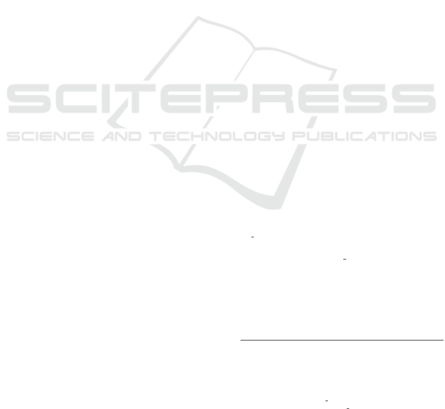
Figure 1: CVH with ﬁre.csv.

small and the large dataset respectively. The trend

in their execution performance does not change be-

tween the small and the large datasets. Overall, Se-

dona’s total execution time is the slowest due to its

considerable data-loading overheads. Yet even focus-

ing on its computational time only, Sedona performs

slower than MASS total execution. This is because

MASS agents converge to a convex hull much faster

than Sedona’s repetitive data shufﬂe-and-sort opera-

tions. Despite that MASS needs to create a 2D Places

space, its total execution time is competitive to MPI or

even better than MPI as increasing the number of ma-

chines beyond eight. This is because MASS can read

input data in parallel while MPI needs to distribute

date from rank 0 to the other worker ranks. Using 18

or 20 machines, Sedona’s shufﬂe-and-sort overheads

diminish, which makes Sedona competitive to MASS.

On the other hand, MASS agent migration over ma-

chine boundary gets increased with more computing

nodes, which slows down MASS execution time be-

yond four machines.

5.2 Euclidean Shortest Path (ESP)

Figures 3 and 4 show all the three libraries’ parallel

performance of ESP execution, each computing with

300 and 500 obstacles respectively. While the small

dataset ranks MASS as the slowest execution, its par-

allel performance continuously improves as increas-

ing the number of machines, which makes MASS the

fastest with 20 computing nodes. The main reason

is that agent propagation actually controls the agent

ICAART 2025 - 17th International Conference on Agents and Artiﬁcial Intelligence

520

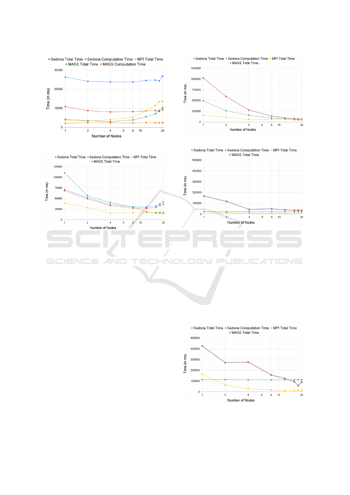
Figure 2: CVH with crime.csv.

Figure 3: ESP with 300Obstacles.txt.

population rather than explodes it since many agents

hit obstacles to stop their propagation. As the number

of computing nodes gets increased, each computing

node has less agents that even alleviate their propaga-

tion. This trend is even clearer with the large dataset

that includes more obstacles. On the other hand, Se-

dona suffers from its Cartesian product computation

that is bound to O(n

). This quadratic complexity

also slows down Sedona’s total execution with the

larger dataset, while still showing its parallel perfor-

mance. MPI’s visibility graph construction similarly

increases quadratic to the data size, but its total ex-

ecution time is the fastest until 16 computing nodes

as each computation of line intersections is computa-

tionally negligible.

5.3 Largest Empty Circle (LEC)

As described in Section 4.3, Sedona, MASS, and

MPI take the same LEC parallelization strategy. Yet,

MASS does not improve parallel performance as its

main() function is the focal point that chooses the

ﬁnal LEC among all potential LECs, each reported

from a different place element. Figures 5 and 6 show

that MASS parallel performance is always bound to

its main() function and does not change. Sedona runs

Figure 4: ESP with 500Obstacles.txt.

Figure 5: LEC with school.csv.

the slowest with 1-12 computing nodes even with the

large dataset but eventually outperforms MASS. This

is because Sedona’s lambda expressions repetitively

compare each pair of potential LECs, which incurs

large overheads with less computing nodes. However,

since Sedona has no focal point in parallelization, its

performance is improved with more machines added

to the computation. Finally, MPI serves as the best

baseline performance as its computation is coarsely

performed in each rank and a one-time reductive com-

munication takes only at the end of the execution to

ﬁnd the ﬁnal result among up to 20 potential LECs.

Figure 6: LEC with s.txt (random points).

Agent-Based Computational Geometry

521

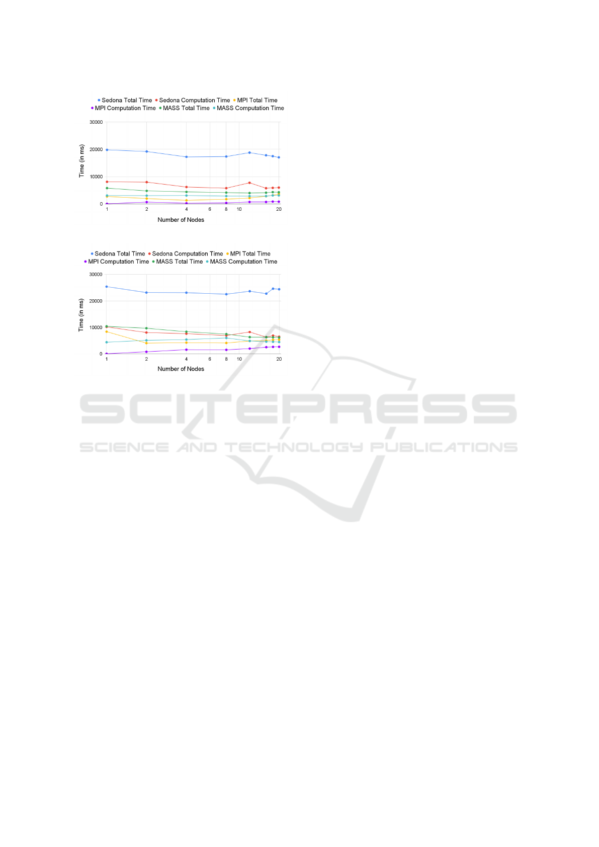
Figure 7: RGS with ﬁre.csv.

Figure 8: RGS with crime.csv.

5.4 Range Search (RGS)

Figures 7 and 8 measure the KD-tree construction and

range-query execution time elapsed by the three li-

braries, as feeding the USFS ﬁre occurrence dataset

(581,541 points) and the LA crime location dataset

(938,458 points). MPI runs the fastest in both cases

while its query transactions, (i.e., MPI computation

time) receive more communication overheads when

increasing the number of machines. On the other

hand, Sedona always runs the slowest. Its main over-

head (which occupies 59% through 73% of the total

time) is its tree construction and results from Sedona’s

repetitive RDD shufﬂe-and-sort operations. These

operations also slow down query transactions in both

small and large datasets, each spending 2.6-1.9 times

and 2.3-1.4 times more than MASS query transac-

tions. MASS cannot outperform MPI while its total

execution time gets closer to MPI’s as increasing the

number of computing nodes beyond 16.

6 CONCLUSIONS

We parallelized four benchmark programs including

CVH, ESP, LEC, and RGS, using MASS, Sedona,

and MPI for the purpose of programmability and per-

formance comparisons. Sedona lines up major built-

in functions in computational geometry, which facil-

itates benchmark programming most efﬁciently. On

the other hand, MASS allows us to code the programs

from the viewpoint of spatial cognition, which makes

them easier to understand than MPI. While MPI runs

fastest in general due to its lowest-level paralleliza-

tion, MASS outperforms Sedona in most benchmark

programs. This demonstrates that agent ﬂocking and

tree traversing are effective in GIS parallel execution.

ACKNOWLEDGMENTS

This paper is dedicated to Dr. Christian Freksa, a

former director of Bremen Spatial Cognition Center,

who gave us valuable hints on computational geom-

etry from the viewpoints of spatial cognition. This

research was supported by IEEE CS Diversity and In-

clusion Fund (IEEE CS D&I, 2023).

REFERENCES

Eldawy, A. and Mokbel, M. F. (2015). SpatialHadoop: A

MapReduce Framework for Spatial Data. In IEEE

31st International Conference on Data Engineering,

pages 1352–1363, Seoul, Korea. IEEE.

Freksa, C., Barkowsky, T., Falomir, Z., and van de Ven, J.

(2019). Geometric problem solving with strings and

pins. Spatial Cognition & Computation, 19(1):46–64.

IEEE CS D&I (2023). New Diversity and Inclusion Projects

Fund. 15 Feb. 2023 | D&I, DEI, Education, Focus35.

North, M. J., Tatara, E., Collier, N., and Ozik, J. (2007).

Visual Agent-based Model Development with Repast

Simphony. In Agent 2007 Conference on Complex In-

teraction and Social Emergence, Chicago, IL.

Spark GraphX (2018). Accessed on: November 2, 2024.

[Online]. Available: https://spark.apache.org/graphx/.

Sullivan, K., Coletti, M., and Luke, S. (2010). GeoMason:

Geospatial Support for MASON. Technical Report

GMU-CS-TR-2016-16, George Mason University.

Wilensky, U. (2013). NetLogo NW Extension, ac-

cessed on: October 5, 2023. [online]. available:

http://ccl.northwestern.edu/netlogo/5.0/docs/nw.html.

Yu, J., Zhang, Z., and Sarwat, M. (2019). Spatial data man-

agement in apache spark: the GeoSpark perspective

and beyond. Geoinformatica, 23(1):37–78.

ICAART 2025 - 17th International Conference on Agents and Artiﬁcial Intelligence

522