Machine Learning Methods for Phenotype Prediction from
High-Dimensional, Low Population Aquaculture Data
Giovanni Faldani
1
, Enrico Rossignolo
1
, Eleonora Signor
1
, Alessio Longo
2
, Sara Faggion
2
,
Luca Bargelloni
2
, Matteo Comin
1
and Cinzia Pizzi
1
1
Department of Information Engineering, University of Padova, Padova, 35131, Italy
2
Department of Comparative Biomedicine and Food Science, University of Padova, Legnaro (PD), 35020, Italy
Keywords:
High-Dimensional, Low Population, SNP Data, Machine Learning Classification, Phenotype Prediction.
Abstract:
Recent research has increasingly focused on classification rules within the big data framework, yet many bioin-
formatics applications still address prediction problems that involve small-sample, high-dimensional data. In
phenotype prediction, especially with the rise of large-scale genomic data, a central challenge arises from han-
dling high-dimensional datasets where the number of genetic features (such as SNPs) far exceeds the sample
size. A significant example of such high-dimensional, low-sample datasets is found in aquaculture, a rapidly
growing sector within global food production and a crucial source of high-quality protein. This study uses data
from an experiment performed on European seabass as a test case, focusing on predicting resistance to Viral
Nervous Necrosis (VNN) as a specific phenotype of interest. We explore a range of machine learning tech-
niques to address the complexities of high-dimensional data, from established methods like gradient boosting,
SVM, and deep learning to newer approaches. This paper evaluates various methods for associating SNPs
with phenotypic traits, benchmarking their performance on challenging aquaculture genomic data to provide
insight into the effectiveness of these techniques.
1 INTRODUCTION
The exploration of genotype-phenotype relationships
has seen a growing number of studies focused
on identifying genetic variants linked to various
diseases. Most single nucleotide polymorphisms
(SNPs), which are used as markers for specific ge-
nomic regions, exert minimal biological effects. To
find the SNPs that impact biological functions is in
general very challenging (Uffelmann et al., 2021).
In recent years, genome-wide association stud-
ies (GWAS) have significantly expanded our under-
standing of SNP roles and associations, shedding light
on the genetic impact on diseases (Uffelmann et al.,
2021). Through GWAS, SNPs can be identified as
candidate biomarkers, potentially indicating suscepti-
bility to complex diseases. Despite GWAS’ success
in pinpointing disease-related SNPs, unique chal-
lenges arise, particularly in the context of big genomic
data where high-dimensional datasets often feature
far more genetic variables than samples (Uppu et al.,
2018). A tightly related problem is the phenotype pre-
diction of a disease from this high-dimensional, low-
population SNP data. In phenotype prediction, where
uncovering gene-disease associations is key, datasets
typically contain a vast number of SNPs (e.g. 10
6
)
against relatively small sample sizes (e.g. 10
3
). Nav-
igating this high-dimensional space to identify rep-
resentative SNPs is a persistent challenge in under-
standing the genetic foundations of disease.
In this paper, we will use as a test case data from
an experimental challenge test performed on Euro-
pean sea bass, and in particular the prediction of a
specific phenotype, resistance to viral nervous necro-
sis (VNN).
Aquaculture is a key source of high-quality pro-
tein worldwide and has become one of the fastest-
growing sectors in global food production (Buri
´
c
et al., 2020; You et al., 2020). European sea bass is a
highly valued species across Europe and the Mediter-
ranean area, carrying substantial economic and cul-
tural importance (Vandeputte et al., 2019). In the past
two decades, global aquaculture production of Euro-
pean sea bass has seen a significant growth, rising
from 7,694 tons in 2000 to 299,810 tons in 2021.
However, the industry faces increasing challenges
from infectious diseases, which threaten both the sus-
tainability of sea bass farming and the health of cul-
638
Faldani, G., Rossignolo, E., Signor, E., Longo, A., Faggion, S., Bargelloni, L., Comin, M. and Pizzi, C.
Machine Learning Methods for Phenotype Prediction from High-Dimensional, Low Population Aquaculture Data.
DOI: 10.5220/0013248000003911
Paper published under CC license (CC BY-NC-ND 4.0)
In Proceedings of the 18th International Joint Conference on Biomedical Engineering Systems and Technologies (BIOSTEC 2025) - Volume 1, pages 638-646
ISBN: 978-989-758-731-3; ISSN: 2184-4305
Proceedings Copyright © 2025 by SCITEPRESS – Science and Technology Publications, Lda.

tured populations.
Viral Nervous Necrosis is a major viral disease
impacting global aquaculture, affecting numerous
farmed and ecologically vital species. It is the pri-
mary viral infectious disease in European sea bass, re-
sponsible for 15% of all on-farm disease-related mor-
talities (Muniesa et al., 2020). VNN resistance in Eu-
ropean sea bass is characterized by significant addi-
tive genetic variation and recently one genomic re-
gion has been detected as significantly associated with
this trait (Mukiibi et al., 2024), yet the specific causal
gene(s) and mutation(s) underlying this resistance re-
main unknown.
In this paper, we exploit three different machine
learning approaches to predict VNN resistance of
about a thousand individuals through the analysis of
several SNPs datasets. Machine learning provides
a versatile and extensive set of techniques suited to
tackle the challenges of these high-dimensional low-
population SNP datasets. Among the several machine
learning approaches, we selected XGBoost (Chen
and Guestrin, 2016), and COMBI (both SVM and
Deep Learning versions) (Mieth et al., 2016; Mi-
eth et al., 2021). Moreover, we designed an ad-hoc
Chaos Game Representation (CGR) approach (Jef-
frey, 1990) that maps sequences of SNPs into im-
ages which are then classified using a Convolutional
Neural Network. This choice of tools covers both
“classic” machine learning approaches (such as SVM
and gradient boosting) and more recent deep learn-
ing approaches, including an original CGR encoding
scheme for SNPs. In our experiments, we assessed
these machine learning methods for SNP and pheno-
type association and evaluated their prediction per-
formance on a challenging bank of high dimensional
aquacultural genomic data to provide insight on their
efficacy and efficiency.
2 METHODS
Our research aims to investigate the mortality of a
low-rank sea bass population exploiting the high di-
mensionality of its SNP data. SNPs act as biological
markers and can identify genes associated with a dis-
ease.
We dig into different machine learning approaches
from boosted trees to support vector machines and
neural networks. Among these, we chose two well-
known machine learning algorithms already applied
in bioinformatics for classifying SNP data: XG-
Boost and COMBI, both characterized by great model
explainability and classification performance. Fur-
thermore, we introduce a novel approach for clas-
sifying SNPs by adapting Chaos Game Representa-
tion (CGR), an alignment-free sequence algorithm, to
make it suitable for representing SNPs. The obtained
representation is then fed to a network of machine
learning classifiers. These three approaches will be
presented in the next sections.
2.1 XGBoost
XGBoost (eXtreme Gradient Boosting) is a widely
used and powerful machine learning algorithm based
on the gradient boosting framework (Chen and
Guestrin, 2016). It has gained significant popularity
due to its efficiency, scalability and effectiveness in
a wide variety of data science applications, including
bioinformatics and genomics.
In bioinformatics, XGBoost has been applied in
tasks such as predicting gene expression values (Li
et al., 2019), identifying disease from biomarkers
(Sharma and Verbeke, 2020), and classifying complex
biological data, such as those coming from SNP data
(Medvedev et al., 2022). One of the major advantages
of XGBoost is its ability to handle sparse data effi-
ciently, which is especially useful when dealing with
medical and biological datasets that require data col-
lection, where missing values are common.
The model trained with XGBoost can be easily
and effectively explained. Gradient boosting is based
on decision trees and decision trees themselves are
effortlessly interpretable compared to more complex
models like neural networks. Each decision tree rep-
resents a series of decisions (or splits) based on fea-
ture values, and these decisions can be visually exam-
ined to understand how the model arrives at its predic-
tions. Operationally this means that a feature is rep-
resented as a decision node. Depending on the value
of this feature, the tree branches into two leaves, each
containing a specific value that is added to the model’s
output.
XGBoost’s feature importance scores are used to
rank the most influential features contributing to the
prediction. The ability to quantify feature importance
is one of XGBoost’s strengths, allowing us to interpret
which features have the most significant impact on the
model’s predictions. This capability is often used in
feature selection before training the real model. The
actual model is trained using the plain genotype coded
as an integer vector (see Section 3.1) without any ad-
ditional preprocessing.
2.1.1 Training Parameters
The hyperparameters used for the model were: the
number of trees (ranged from 10 to 100); the grow
Machine Learning Methods for Phenotype Prediction from High-Dimensional, Low Population Aquaculture Data
639

policy (either loss-guide or depth-wise); the learn-
ing rate (ranged from 0.01 to 0.2); the maximum tree
depth (between 4 and 6); the minimum child weight
(between 1 and 3); λ (ranged from 0 to 5); and γ
(ranged from 0 to 5) that can be tuned to add com-
plexity or limit overfitting. The best hyperparameters
are chosen with the help of a grid-search.
2.2 COMBI
The two methods that carry the name COMBI aim at
examining the relation between SNPs and phenotyp-
ical traits (Mieth et al., 2016) and represent the ba-
sis of the interpretable machine learning paradigms in
bioinformatics for the analysis of human DNA. These
paradigms focus on the explainability of certain traits
while still offering predictive capability, and aim at
maximizing both of these aspects of classification.
For this end, COMBI uses a support vector machine
model (Cortes and Vapnik, 1995) applied to the Well-
come Trust Case Control Consortium (WTCCC) data
of human genome-disease association (Jones et al.,
2007), taking advantage of the direct mathematical
correlation it provides between inputs and outputs.
The decision-making process of machine learn-
ing algorithms is usually black-box, limiting the in-
terpretability of results in complex contexts such as
SNP data and other biological data. COMBI has
proved extremely useful in providing an answer to
this problem, like detecting genetic risk scores for
quantifying patients’ predisposition to disease on the
WTCCC (Marigorta et al., 2018), advancing precision
medicine in the field of oncology for therapy targeted
to each patient (Asada et al., 2021), and predicting
susceptibility to asthma based on SNP information of
individuals (Gaudillo et al., 2019).
Recently, deep learning has emerged as a power-
ful classification tool, leading to the development of
DeepCOMBI (Mieth et al., 2021), a neural network-
based classifier that uses layer relevance propagation
to achieve the same level of explainability as the orig-
inal COMBI model, with increased performance on
the same WTCCC dataset. DeepCOMBI has suc-
cessfully been applied to the study of the response
of rheumatoid arthritis patients to certain medication
based on their genome data, helping to better identify
non-responders (Lim et al., 2022), and for improving
risk prediction of developing schizophrenia, a highly
inheritable disorder whose genetic markers are still
unclear (Martins et al., 2024).
In this study, the COMBI framework consists of
the testing and adaptation of the methods used by
COMBI (Mieth et al., 2016) with the Support Vec-
tor Machine (SVM) model and DeepCOMBI (Mieth
et al., 2021) with the Multilayer Perceptron (MLP)
model.
2.2.1 Training Parameters
The following parameters were obtained with a grid-
search selection process, where the search space ex-
tremities are listed in parentheses after the chosen
value.
The hyperparameters used for the SVM model
were: L2 regularization with C = 100 (1, 100) and
squared hinge loss (Lee and Lin, 2013). The SVM
model was trained until convergence and its optimal
hyperparameters were found through a grid-search
procedure.
The hyperparameters used for the MLP model
were: one hidden layer of 128 neurons (128, 512);
0.3 dropout rate between each layer (0.0, 0.5);
ReLU activation function; L1 and L2 regularization
weighted at 0.1 and 0.01 respectively (0.0001, 0.1);
learning rate 10
−12
(10
−14
, 10
−3
) with binary cross-
entropy loss and 1, 000 epochs of training on the data
(100, 1, 000).
2.3 Chaos Game Representation
Chaos Game Representation (CGR) is an iterative
mapping technique to transforms a sequence defined
over an alphabeth Σ into an image. In CGR a se-
quence is represented as a unique pattern and is
mapped to unique coordinates. For any sequence,
regardless of its length and background, CGR can
encode it into an image by representing each fea-
ture through a point identified by coordinates; further-
more, by knowing the coordinates of a feature, CGR
allows the inference of the input sequence.
The application of CGR to bioinformatics was
first proposed in (Jeffrey, 1990), where an encod-
ing scheme for genomic sequences into squares was
first proposed. In this representation each vertex
of the square corresponds to one of the four DNA
nucleotides, with Σ = {A, C, G, T }. Extension to
the framework have followed, involving also RNA,
proteins and physio-chemical properties (Kania and
Sarapata, 2022; Dick and Green, 2020; Akbari
Rokn Abadi et al., 2023).
2.3.1 Encoder Unit
To apply the Chaos Game Representation algorithm
to the context of sea bass genetic data, we modified its
genomic application to genotype sequences. Our pro-
posed CGR encoding for genotype keeps the square
representation assigning a genotype to each of the
vertices except one, for backward compatibility with
BIOINFORMATICS 2025 - 16th International Conference on Bioinformatics Models, Methods and Algorithms
640

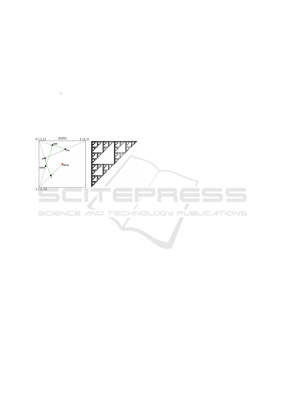
genomic sequences, and maintains the distribution of
genotype s within the image clear (Figure 1).
Let h = h
1
. . . h
n
be a sequence defined over the
alphabet Σ = {0, 1, 2}. Then the CGR encoding of
the sequence h is the bidimensional representation of
the ordered set of pairs {(x
i
, y
i
), 0 ≤ i ≤ n}, where the
pair (x
i
, y
i
) is iteratively defined as:
(x
i
, y
i
) =
1
2
((x
i−1
, y
i−1
) + g(h
i
)) with i ≥ 1 (1)
where the origin O(x
0
, y
0
) = (0, 0) and
g(h
i
) =





(−1, 1) h
i
= 0
(−1, −1) h
i
= 1
(1, 1) h
i
= 2
(2)
Figure 1: The Chaos Game Representation applied to geno-
type sequence. The graphical-conceptual application of
CGR for genotype (Left column) and image conversion for
a sea bass with Active10 SNP features (Right column).
2.3.2 Classifier Unit
Our classifier unit consists of a Deep Convolutional
Neural Network (DCNN). We chose to use DCNN
due to the large number of SNP features selected
against the small number of sea basses in the ana-
lyzed datasets. We instantiated and tested several net-
works: AlexNet (Krizhevsky et al., 2017), ResNet50
and ResNet101 (He et al., 2016).
AlexNet and ResNet are three-channel architec-
tures and require a fixed image size for training;
227 ×227 for AlexNet and 224×224 for ResNet. We
replicated the content of the single channel in each
of the three channels and resized the images, with di-
mensions consistent with networks, using bicubic in-
terpolation (Lundh et al., 2024).
2.3.3 Training Parameters
The hyperparameters used for the model were the last
dense layer with one neuron for the binary classifica-
tion; SGD optimizer with learning rate 10
−3
and the
sparse categorical cross-entropy loss function; 5-fold
cross-validation of training on the data with a number
of epochs from 30 to 120 and batch sizes from 15 to
30, due to the high dimensionality of the SNP features
and the low-rank data treated in this study.
3 EXPERIMENTS AND
DISCUSSION
This section presents the aquaculture data we used in
our research, the experimental setup instantiated on
our classification models, and the phenotype classifi-
cation results we obtained on each model and experi-
ment performed.
3.1 Datasets
Data used in our research refer to the study (Muki-
ibi et al., 2024). In that study, 990 European sea
bass, produced in a full-factorial mating scheme us-
ing 25 sires and 25 dams, were subjected to a 29
days NNV (nervous necrosis virus) challenge test.
Mortality was individually recorded as a binary trait
(alive/dead). Phenotypes were fairly balanced hav-
ing 54.24Sires, dams and 40 offspring were whole-
genome sequenced, whereas the remaining offspring
were genotyped using a commercial SNP array con-
sisting of about 30K SNPs. These animals were
then imputed to whole-genome sequence, obtain-
ing a high-dimensional genotype data consisting of
6,072,853 SNPs for each fish. Since European sea
bass is a diploid organism, it has two alleles at the
SNP and two possible variations from the reference
allele. Genomic data included:
• the SNP feature identifier, composed by chromo-
some number and location of each SNP in base
pairs;
• the number of copies of the reference allele (in
this case, the minor allele), that can be 0, 1 or 2.
Having only 990 samples, the feature matrix is
low-rank, making it exceptionally difficult to analyze.
To overcome the data’s high dimensionality, we
will use three groups of features selected on the basis
of functional genomic information: 1) Tissue specific,
2) Active, and 3) Control. Tissue-specific refers to ge-
netic variants located in open chromatin regions based
on ATAC-seq data obtained from two key tissues in
VNN, brain and head kidney, sampling 10 fish either
after infection or mock-infected. Active refers to ac-
tive regulatory regions based on ATAC- and ChIP-
seq data from several different tissue types (brain,
gill, liver, gonads, skeletal muscle and head kidney)
in control fish. Active datasets consist of SNPs in-
cluded in regulatory regions that were found to be ac-
Machine Learning Methods for Phenotype Prediction from High-Dimensional, Low Population Aquaculture Data
641

tive across at least 80%, 50% and 10% of analysed
tissues. Control datasets, numerically proportional to
the Active ones, contain randomly selected SNP fea-
tures that were located within non-active regions (i.e.
quiescent regions).
Tissue-specific datasets are very large datasets
with a large number of SNPs (about a million); in-
stead, Active and Control datasets have a far fewer
number of SNPs (thousands or tens of thousands),
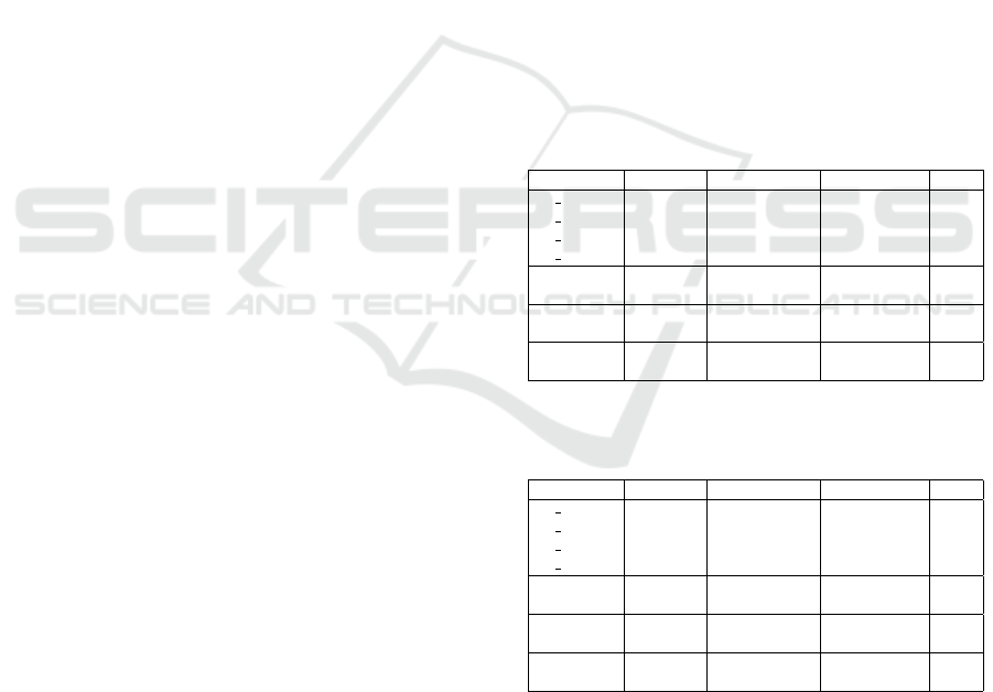
more details are reported in Table 1.
Table 1: Information on the composition of the datasets in
Tissue-specific, Active and Control categories.
Category Dataset # SNPs
Tissue-specific
Hk NNV 1,193,048
Hk mock 1,082,100
Br NNV 775,840
Br mock 832,801
Active
Active80 6,862
Active50 11,130
Active10 80,768
Control
Control80 6,862
Control50 11,130
Control10 80,768
All fish were divided in two genomically distant
populations through key-means clustering (cluster 0
and cluster 1), minimizing intra-class relatedness and
maximizing inter-class genomic distance.
Genomic prediction across genomically divergent
populations represents a significant challenge (Amar-
iuta et al., 2020). The two clusters, each representing
a genomically distant population, were created clas-
sifying each sea bass through genomic information.
Clustering animals on the basis of their genomic re-
lationships within only two clusters implies some ge-
nomic diversification also intra-class, consequence of
the low number of individuals, which does not allow a
complete mapping of relationships within each clus-
ter. Animal clustering into genomically distant popu-
lations and the classification for phenotypes is shown
in Table 2.
Table 2: Distribution of sea basses by genomically distant
populations and phenotypes.
# sea basses
Phenotypes
alive dead
Cluster 0 589 373 216
Cluster 1 401 164 237
Total 990 537 453
3.2 Experimental Setup
We carried out several tests on a random partition and
on the genomically distant population data.
In the random partition test, the data are parti-
tioned using training and testing sets with an 80%-
20% split. Given the high dimensionality of the data,
we used the features selected based on biological
significance. We considered first the Tissue-specific
datasets, which are more extensive. Then we move
to the Active datasets that contain far fewer features
compared to the Tissue-specific ones, helping to as-
sess whether the number of SNPs influences classi-
fication performance. To assess the effectiveness of
the selected SNPs for classification, we compared the
models trained on the Active selections with Control
models using random SNP selections of the same size.
These Control datasets allowed us to verify whether
the SNPs chosen based on biological relevance were
genuinely contributing to improved classification per-
formance.
We also set up the genomically distant population
test. The models were trained on the largest partition
(cluster 0) and tested on the other (cluster 1), since the
largest of the two clusters makes for a more adequate
training set.
Four machine learning models were employed:
XGBoost, COMBI SVM, DeepCOMBI, and CGR.
The models were evaluated using accuracy, precision,
recall, and F1-score.
3.3 Results and Discussion
Here the results obtained by each of the models are
reported, tested on the various splits of data described
above. The main observation to highlight for these
tests is that the task at hand is quite challenging, as
we know the mortality phenotype taken in exam is
not exclusively determined by the genotype, so all re-
sults reflect this difficulty. This section will only list
the F1-score as a performance metric for space limi-
tations, but the complete set of results can be found in
the Supplemental Material.
3.3.1 Random Partition Tests
The first benchmark used was a random fixed 80%
training and 20% test partition for the individuals in
the Tissue-specific datasets, as is standard practice in
many machine learning applications and tasks. Tests
on this split are a useful metric to compare the effi-
cacy of these approaches with regard to the rest of the
literature on the subject, minding the challenge of the
data at hand. The results of these tests are listed in
Table 3.
BIOINFORMATICS 2025 - 16th International Conference on Bioinformatics Models, Methods and Algorithms
642

Table 3: F1-scores obtained on the Tissue-specific tests us-
ing the random partition split.
Dataset XG-
Boost
COMBI
SVM
Deep-
COMBI
CGR
Hk NNV 0.53 N/A 0.53 0.15
Hk mock 0.53 N/A 0.61 0.58
Br NNV 0.58 0.62 0.61 0.58
Br mock 0.58 0.62 0.48 0.26
Note that the COMBI SVM method uses the un-
derlying LIBLINEAR (Fan et al., 2008) software li-
brary for its implementation, which has a maximum
allowed variable size that is exceeded by the amount
of data in the head-kidney tissues.
The best performance we were able to achieve on
the random partition tests is using the COMBI SVM
approach on the sets that allowed it, reaching 62%
F1-score, while the head-kidney datasets have proven
more challenging for XGBoost. Both of the neural
network-based DeepCOMBI and CGR methods en-
counter significantly more difficulty in the Hk NNV
and Br mock datasets, but achieve 61% and 58% F1-
score respectively on Hk mock and Br NNV.
The head-kidney and brain tissue data contain an
extremely large number of SNPs, since all four data
sets represent accessible, but not necessarily active
genomic regions. As a means to significantly re-
duce the number of features, we decided to use more
detailed functional information, including ChIP/seq
data. This allowed to identify active regulatory ele-
ments. Despite the inclusion of a larger number of tis-
sues, focusing on active regions only enabled a dras-
tic reduction of features, while preserving core in-
formation on biological importance. This way, three
datasets containing Active SNPs were tested. To as-
certain the quality of these selections, randomly sam-
pled datasets of the same size were used as Control
sets, with the expectation that the Active SNP selec-
tions would yield higher performance than the Con-
trol sets because of their careful filtering process. The
comparison of the above tests using the same random
fixed 80%-20% split as above can be found in Table
4.
Table 4: F1-scores obtained on the Active and Control tests
using the random partition split.
Dataset XG-
Boost
COMBI
SVM
Deep-
COMBI
CGR
Active80 0.60 0.62 0.42 0.58
Control80 0.51 0.63 0.00 0.10
Active50 0.57 0.60 0.62 0.48
Control50 0.57 0.61 0.04 0.40
Active10 0.58 0.62 0.53 0.52
Control10 0.61 0.63 0.39 0.00
The tests using Active and Control subsets re-
veal how each model is able to distinguish between
high-quality SNP data and random noise. XGBoost
seems to distinguish well between Active80 and Con-
trol80, but loses this ability on the 50% and 10%
variants, while COMBI SVM seems to be unable to
make meaningful distinctions between any couple of
Active and Control sets. Interestingly, both of the
neural network-based approaches display huge gaps
in F1-score between Active and Control sets, often
with many decimal points of difference. This would
suggest that these methods are better suited at distin-
guishing the random noise of the control sets from
more meaningful SNP data.
3.3.2 Genomically Distant Population Tests
The results of the tests performed using the parti-
tion of genomically distant individuals in clusters are
summed up in Table 5. The clusters were selected to
be as genomically distant from each other as possi-
ble, making the expectation for this task to be worse
overall performance than the random partition tests.
In these tests, the COMBI SVM framework was able
to process all data due to the smaller training sets.
Table 5: F1-scores obtained on the Tissue-specific tests us-
ing the genomically distant split.
Dataset XG-
Boost
COMBI
SVM
Deep-
COMBI
CGR
Hk NNV 0.60 0.41 0.09 0.40
Hk mock 0.49 0.41 0.34 0.00
Br NNV 0.59 0.42 0.71 0.31
Br mock 0.51 0.41 0.46 0.67
On these data splits we can see how, as expected,
the difficulty of the problem notably increases, due to
the much smaller training set size and groups specifi-
cally selected in a way to contain genomically differ-
ent individuals, making the prediction of the pheno-
type overall much harder. In spite of this, some re-
sults go even beyond what the 80%-20% tests were
able to achieve, with markedly high F1-scores of
60% on Hk NNV by XGBoost, 71% on Br NNV by
DeepCOMBI, and 67% on Br mock by CGR. The
Hk mock dataset becomes very challenging for all
methods, and COMBI SVM performs badly on all
Tissue-specific datasets.
Lastly, the same genomically distant test was per-
formed as before on the Active and Control datasets,
listed in Table 6. Using these clusters, the Active and
Control tests also show more ambiguous results than
before. On the 80% sets, all methods except COMBI
SVM struggle to distinguish between the random and
meaningful data, while the 50% sets show good dis-
Machine Learning Methods for Phenotype Prediction from High-Dimensional, Low Population Aquaculture Data
643

Table 6: F1-scores obtained on the Active and Control tests
using the genomically distant split.
Dataset XG-
Boost
COMBI
SVM
Deep-
COMBI
CGR
Active80 0.58 0.50 0.25 0.62
Control80 0.63 0.43 0.44 0.74
Active50 0.66 0.49 0.70 0.74
Control50 0.62 0.43 0.42 0.55
Active10 0.64 0.42 0.72 0.76
Control10 0.61 0.39 0.68 0.74
criminatory capabilities on all models, with gaps of
many decimal points between Active and Control.
Active10 and Control10 are interestingly only a few
decimal points apart on every test, but with Active10
always in the lead, giving the impression that there
is just enough difference to meaningfully distinguish
the two. When it comes to overall classification per-
formance, the CGR model outperforms all the other
ones on the Active sets, often nearing or exceeding
70% F1-score, indicating that despite the diversity of
the clusters, there are features highlighted by the CGR
representation that can meaningfully distinguish be-
tween the two phenotypes very well.
4 CONCLUSIONS
In summary, XGBoost does not often perform the
best, but among all models it is the one that most
consistently obtained reliable results often reaching
around 60% F1-score on all the above tests. COMBI
SVM reaches a similar level of reliability on the 80%-
20% split tests, but it finds significantly more diffi-
culty in classification between the two clusters, while
DeepCOMBI’s performance is inconsistent, ranging
from very good at over 70% F1-score, to extremely
poor at under 10%. CGR is similarly inconsistent
in most cases, with high peaks and low valleys, but
shines when used on the Active splits for the genomi-
cally distant population tests.
ACKNOWLEDGMENTS
Authors are supported by the Project funded under
the National Recovery and Resilience Plan (NRRP),
Mission 4 Component 2 Investment 1.4 - Call for
tender No. 3138 of 16 December 2021, rectified by
Decree n.3175 of 18 December 2021 of Italian Min-
istry of University and Research funded by the Euro-
pean Union – NextGenerationEU; Project code CN-
00000033, Concession Decree No. 1034 of 17 June
2022 adopted by the Italian Ministry of University
and Research, CUP D33C22000960007, Project title
“National Biodiversity Future Center - NBFC”.
REFERENCES
Akbari Rokn Abadi, S., Mohammadi, A., and Koohi, S.
(2023). A new profiling approach for dna sequences
based on the nucleotides’ physicochemical features
for accurate analysis of sars-cov-2 genomes. BMC ge-
nomics, 24(1):266.
Amariuta, T., Ishigaki, K., Sugishita, H., Ohta, T., Koido,
M., Dey, K., Matsuda, K., Murakami, Y., Price,
A., Kawakami, E., Terao, C., and Raychaudhuri, S.
(2020). Improving the trans-ancestry portability of
polygenic risk scores by prioritizing variants in pre-
dicted cell-type-specific regulatory elements. Nature
Genetics, 52:1–9.
Asada, K., Kaneko, S., Takasawa, K., Machino, H., Taka-
hashi, S., Shinkai, N., Shimoyama, R., Komatsu, M.,
and Hamamoto, R. (2021). Integrated analysis of
whole genome and epigenome data using machine
learning technology: toward the establishment of pre-
cision oncology. Frontiers in oncology, 11:666937.
Buri
´
c, M., Bav
ˇ
cevi
´
c, L., Grguri
´
c, S., Vresnik, F., Kri
ˇ
zan, J.,
and Antoni
´
c, O. (2020). Modelling the environmen-
tal footprint of sea bream cage aquaculture in relation
to spatial stocking design. Journal of Environmental
Management, 270:110811.
Chen, T. and Guestrin, C. (2016). Xgboost: A scalable
tree boosting system. In Proceedings of the 22nd acm
sigkdd international conference on knowledge discov-
ery and data mining, pages 785–794.
Cortes, C. and Vapnik, V. (1995). Support-vector networks.
Mach. Learn., 20(3):273–297.
Dick, K. and Green, J. R. (2020). Chaos game representa-
tions & deep learning for proteome-wide protein pre-
diction. In 2020 IEEE 20th International Conference
on Bioinformatics and Bioengineering (BIBE), pages
115–121.
Fan, R. E., Chang, K. W., Hsieh, C. J., Wang, X. R., and
Lin, C. J. (2008). Liblinear: A library for large linear
classification. J. Mach. Learn. Res., 9:1871–1874.
Gaudillo, J., Rodriguez, J. J. R., Nazareno, A., Baltazar,
L. R., Vilela, J., Bulalacao, R., Domingo, M., and
Albia, J. (2019). Machine learning approach to sin-
gle nucleotide polymorphism-based asthma predic-
tion. PLOS ONE, 14(12):1–12.
He, K., Zhang, X., Ren, S., and Sun, J. (2016). Deep resid-
ual learning for image recognition. In 2016 IEEE Con-
ference on Computer Vision and Pattern Recognition
(CVPR), pages 770–778.
Jeffrey, H. (1990). Chaos game representation of gene struc-
ture. Nucleic Acids Research, 18(8):2163–2170.
Jones, R. W., McArdle, W. L., Ring, S. M., Strachan, D. P.,
Pembrey, M., Clayton, D. G., Dunger, D. B., Nutland,
S., Stevens, H. E., Walker, N. M., Widmer, B., Todd,
J. A., et al. (2007). Genome-wide association study
of 14,000 cases of seven common diseases and 3,000
shared controls. Nature, 447(7145):661–678.
BIOINFORMATICS 2025 - 16th International Conference on Bioinformatics Models, Methods and Algorithms
644

Kania, A. and Sarapata, K. (2022). Multifarious aspects of
the chaos game representation and its applications in
biological sequence analysis. Computers in Biology
and Medicine, 151:106243.
Krizhevsky, A., Sutskever, I., and Hinton, G. E. (2017). Im-
agenet classification with deep convolutional neural
networks. Commun. ACM, 60(6):84–90.
Lee, C. P. and Lin, C. J. (2013). A study on l2-loss
(squared hinge-loss) multiclass svm. Neural Compu-
tation, 25(5):1302–1323.
Li, W., Yin, Y., Quan, X., and Zhang, H. (2019). Gene ex-
pression value prediction based on xgboost algorithm.
Frontiers in Genetics, 10.
Lim, A. J., Lim, L. J., Ooi, B. N., Koh, E. T., Tan, J. W. L.,
Chong, S. S., Khor, C. C., Tucker-Kellogg, L., Leong,
K. P., and Lee, C. G. (2022). Functional coding haplo-
types and machine-learning feature elimination identi-
fies predictors of methotrexate response in rheumatoid
arthritis patients. EBioMedicine, 75.
Lundh, F., Clark, J. A., and contributors (2024). Image
module - pillow (pil fork) 10.4.0 documentation. Last
consultation 23 September 2024.
Marigorta, U. M., Rodr
´
ıguez, J. A., Gibson, G., and
Navarro, A. (2018). Replicability and prediction:
Lessons and challenges from gwas. Trends in Genet-
ics, 34(7):504–517.
Martins, D., Abbasi, M., Egas, C., and Arrais, J. P. (2024).
Enhancing schizophrenia phenotype prediction from
genotype data through knowledge-driven deep neural
network models. Genomics, 116(5):110910.
Medvedev, A., Mishra Sharma, S., Tsatsorin, E., Nabieva,
E., and Yarotsky, D. (2022). Human genotype-to-
phenotype predictions: Boosting accuracy with non-
linear models. PloS one, 17(8):e0273293.
Mieth, B., Kloft, M., Rodr
´
ıguez, J. A., Sonnenburg, S., Vo-
bruba, R., Morcillo-Su
´
arez, C., Farr
´
e, X., Marigorta,
U. M., Fehr, E., Dickhaus, T., et al. (2016). Combin-
ing multiple hypothesis testing with machine learning
increases the statistical power of genome-wide associ-
ation studies. Scientific reports, 6(1):36671.
Mieth, B., Rozier, A., Rodriguez, J. A., H
¨
ohne, M. M. C.,
G
¨
ornitz, N., and M
¨
uller, K.-R. (2021). DeepCOMBI:
explainable artificial intelligence for the analysis and
discovery in genome-wide association studies. NAR
Genomics and Bioinformatics, 3(3):lqab065.
Mukiibi, R., Ferraresso, S., Franch, R., Peruzza, L., Ro-
vere, G. D., Babbucci, M., Bertotto, D., Toffan, A.,
Pascoli, F., Faggion, S., Pe
˜
naloza, C., Tsigenopoulos,
C. S., Houston, R. D., Bargelloni, L., and Robledo, D.
(2024). Integrated functional genomic analysis identi-
fies the regulatory variants underlying a major qtl for
disease resistance in european sea bass. bioRxiv.
Muniesa, A., Basurco, B., Aguilera, C., Furones, D., Re-
vert
´
e, C., Sanjuan-Vilaplana, A., Jansen, M. D., Brun,
E., and Tavornpanich, S. (2020). Mapping the knowl-
edge of the main diseases affecting sea bass and sea
bream in mediterranean. Transboundary and Emerg-
ing Diseases, 67(3):1089–1100.
Sharma, A. and Verbeke, W. J. M. I. (2020). Improving
diagnosis of depression with xgboost machine learn-
ing model and a large biomarkers dutch dataset (n =
11,081). Frontiers in Big Data, 3.
Uffelmann, E., Huang, Q., Munung, N., De Vries, J.,
Okada, Y., Martin, A., Martin, H., Lappalainen, T.,
and Posthuma, D. (2021). Genome-wide association
studies. Nature Reviews Methods Primers, 1:1–21.
Uppu, S., Krishna, A., and Gopalan, R. P. (2018). A
review on methods for detecting snp interactions in
high-dimensional genomic data. IEEE/ACM Transac-
tions on Computational Biology and Bioinformatics,
15:599–612.
Vandeputte, M., Gagnaire, P.-A., and Allal, F. (2019). The
european sea bass: a key marine fish model in the wild
and in aquaculture. Animal Genetics, 50(3):195–206.
You, X., Shan, X., and Shi, Q. (2020). Research advances in
the genomics and applications for molecular breeding
of aquaculture animals. Aquaculture, 526:735357.
APPENDIX
Supplemental Material
Table 7: Accuracy scores obtained using the random parti-
tion split.
Accuracy XGBoost COMBI SVM DeepCOMBI CGR
Hk NNV 0.58 N/A 0.53 0.55
Hk mock 0.58 N/A 0.46 0.53
Br NNV 0.64 0.66 0.60 0.56
Br mock 0.62 0.66 0.57 0.55
Active80 0.65 0.65 0.55 0.59
Control80 0.57 0.67 0.53 0.54
Active50 0.61 0.64 0.48 0.56
Control50 0.64 0.65 0.55 0.56
Active10 0.60 0.66 0.49 0.65
Control10 0.61 0.66 0.52 0.53
Table 8: Accuracy scores obtained using the genomically
distant split.
Accuracy XGBoost COMBI SVM DeepCOMBI CGR
Hk NNV 0.58 0.52 0.41 0.47
Hk mock 0.52 0.52 0.43 0.41
Br NNV 0.55 0.53 0.55 0.45
Br mock 0.49 0.53 0.45 0.56
Active80 0.55 0.56 0.45 0.56
Control80 0.60 0.54 0.46 0.59
Active50 0.61 0.57 0.56 0.59
Control50 0.57 0.53 0.49 0.53
Active10 0.59 0.53 0.57 0.66
Control10 0.57 0.52 0.55 0.59
Machine Learning Methods for Phenotype Prediction from High-Dimensional, Low Population Aquaculture Data
645

Table 9: Precision scores obtained using the random parti-
tion split.
Precision XGBoost COMBI SVM DeepCOMBI CGR
Hk NNV 0.58 N/A 0.49 1.00
Hk mock 0.55 N/A 0.46 0.50
Br NNV 0.62 0.63 0.55 0.52
Br mock 0.59 0.63 0.54 0.45
Active80 0.64 0.62 0.51 0.56
Control80 0.54 0.64 0.00 0.45
Active50 0.58 0.62 0.47 0.52
Control50 0.63 0.63 0.50 0.54
Active10 0.56 0.63 0.46 0.66
Control10 0.57 0.64 0.46 0.00
Table 10: Precision scores obtained using the genomically
distant split.
Precision XGBoost COMBI SVM DeepCOMBI CGR
Hk NNV 0.68 0.76 0.52 0.61
Hk mock 0.65 0.75 0.55 0.00
Br NNV 0.64 0.77 0.58 0.61
Br mock 0.59 0.77 0.54 0.60
Active80 0.64 0.77 0.65 0.64
Control80 0.70 0.78 0.57 0.60
Active50 0.68 0.81 0.58 0.59
Control50 0.64 0.75 0.63 0.63
Active10 0.66 0.78 0.59 0.65
Control10 0.66 0.78 0.58 0.59
Table 11: Recall scores obtained using the random partition
split.
Recall XGBoost COMBI SVM DeepCOMBI CGR
Hk NNV 0.59 N/A 0.57 0.01
Hk mock 0.51 N/A 0.90 0.73
Br NNV 0.55 0.62 0.68 0.65
Br mock 0.57 0.62 0.44 0.15
Active80 0.56 0.62 0.35 0.55
Control80 0.49 0.62 0.00 0.05
Active50 0.56 0.58 0.91 0.43
Control50 0.53 0.59 0.01 0.32
Active10 0.59 0.60 0.62 0.51
Control10 0.65 0.62 0.34 0.00
Table 12: Recall scores obtained using the genomically dis-
tant split.
Recall XGBoost COMBI SVM DeepCOMBI CGR
Hk NNV 0.54 0.28 0.05 0.30
Hk mock 0.39 0.29 0.25 0.00
Br NNV 0.54 0.29 0.92 0.21
Br mock 0.45 0.28 0.40 0.77
Active80 0.53 0.37 0.15 0.60
Control80 0.57 0.30 0.36 0.96
Active50 0.65 0.35 0.88 0.99
Control50 0.59 0.30 0.32 0.49
Active10 0.62 0.29 0.90 0.90
Control10 0.56 0.26 0.82 1.00
BIOINFORMATICS 2025 - 16th International Conference on Bioinformatics Models, Methods and Algorithms
646