Modelling Defence Planning as a Sequential Decision Problem
Carolyn Chen
a
, Mark Rempel
b
and Kendall Wheaton
Centre for Operational Research and Analysis, Defence Research and Development Canada,
60 Moodie Dr., Ottawa, Canada
Keywords:
Defence Planning, Sequential Decision Problem, Mathematical Modelling, Military.
Abstract:
Defence planning in a nation’s defence organization is a complex process that requires considering hundreds
of projects and billions of taxpayer dollars. While a variety of methods, such as integer programming and
genetic algorithms, are used in practice to help decision makers select in which projects to invest, their appli-
cation tends to not account for the fact that these decisions are made sequentially and under uncertainty. In this
paper, we present the first steps towards developing a sequential decision model of the Canadian Department
of National Defence’s multi-gate Project Approval Process that addressed both issues. Our contributions are
twofold. First, using the universal modelling framework for sequential decisions we present a mathematical
model that accounts for the sequential nature of project selection, arrival of new projects over time, and un-
certainty in future budgets. In addition, we extend this model to account for the uncertainty in how a project’s
cost changes over time when its selection is delayed. Second, we demonstrate how these models may be
used to compare the effectiveness of three project selection decision policies, namely a ranked list approach, a
knapsack approach, and a knapsack approach that reserves a contingency fund for future projects.
1 INTRODUCTION
Defence planning is a critical activity that aims to
help nations achieve both their short- and long-term
defence and security objectives. However, selecting
the right capabilities, and thus projects, in which to
invest is not always a straightforward process. This
is due to a variety of factors—financial constraints,
regulatory constraints, multiple conflicting objectives,
interdependence between projects, cost uncertainty,
etc.—that often introduce a high-degree of complex-
ity to the selection process. In addition, the planning
process often must consider various project types si-
multaneously, including those focused on information
technology, equipment, infrastructure, as well as sup-
port contracts (Rempel and Young, 2017). As a result,
the project delivery timelines considered may vary
significantly. For example, the Canadian Defence In-
vestment Plan 2018 included projects with both near-
and long-term delivery dates ranging from 2022 to
2038 (Government of Canada, 2019).
In order to accommodate the wide range of time-
lines, planning processes “must consider a temporal
dimension including immediate activities to possible
a
https://orcid.org/0000-0003-0209-1666
b
https://orcid.org/0000-0002-6248-1722
demands a few decades into the future”, and as a re-
sult occur in “an inherently uncertain and often un-
stable external environment where defence organisa-
tions are required to reorganise for, and respond to,
unpredicted turns of events” (Filinkov and Dortmans,
2014, p. 76). With this in mind, many defence plan-
ning problems may be aptly described as sequential
decision making problems under uncertainty. Fur-
thermore, when decision makers are seeking a port-
folio, the defence planning problem may be described
as a multi-period portfolio optimization problem (Salo
et al., 2024) and modelled as a knapsack problem (Lo-
catelli, 2023).
The classic approach to solve a sequential deci-
sion problem is to model it as a Markov Decision
Process (MDP) (Puterman, 2005) and use Dynamic
Programming (DP) (Bellman, 1957) to find a decision
policy—“a rule (or function) that determines a deci-
sion given the information available” (Powell, 2011,
p. 221)—that makes decisions which result in the sys-
tem performing optimally with respect to a given cri-
terion or objective. However, in many real-world sit-
uations this is not feasible due to the curse of dimen-
sionality (Kuo and Sloan, 2005) and the curse of mod-
elling (Bertsekas and Tsitsiklis, 1996).
Given these limitations, alternative approaches
such as linear programming (and its variants—integer
156
Chen, C., Rempel, M. and Wheaton, K.
Modelling Defence Planning as a Sequential Decision Problem.
DOI: 10.5220/0013248200003893
Paper copyright by his Majesty the King in Right of Canada as represented by the Minister of National Defence
In Proceedings of the 14th International Conference on Operations Research and Enterprise Systems (ICORES 2025), pages 156-164
ISBN: 978-989-758-732-0; ISSN: 2184-4372
Proceedings Copyright © 2025 by SCITEPRESS – Science and Technology Publications, Lda.

programming, mixed-integer programming, etc.), ge-
netic algorithms, tabu search, and other novel heuris-
tics have been used to provide decision support. This
is evidenced by a recent review of 54 application-
based articles that described the use of such ap-
proaches for portfolio optimization in a defence con-
text (Harrison et al., 2020, see Table 1). Further anal-
ysis of these articles reveals that while many address
sources of uncertainty in their respective problems,
only five articles (Crawford et al., 2003; Tsaganea,
2005; Fisher et al., 2015; Shafi et al., 2017; Moallemi
et al., 2018) account for both uncertainty and new
arriving projects which are selected for investment
over time—thus, modelling their respective problems
as sequential decision problems. Inspired by Fisher
et al. (2015), who studied a capital investment plan-
ning problem in the context of the Royal Canadian
Navy, this paper presents the first steps towards de-
veloping a sequential decision model of the Canadian
Department of National Defence (DND)’s multi-gate
Project Approval Process (PAP).
This paper’s main contributions are twofold. First,
using the universal modelling framework for sequen-
tial decisions (Powell, 2022), two sequential deci-
sion models are presented: (i) a model that accounts
for the sequential nature of project selection, the ar-
rival of new projects over time, and uncertainty in fu-
ture budgets; and (ii) an extension of the first model
which incorporates the uncertainty in how a project’s
cost changes over time when its selection is delayed.
Both the uncertainty in the future years’ budgets and
changes in a project’s costs were not represented in
Fisher et al. (2015), and thus this paper extends the
existing research in terms of modelling. Second, we
demonstrate how these models may be used to com-
pare the effectiveness of three project selection deci-
sion policies, namely a ranked list approach, a knap-
sack approach, and a knapsack approach that reserves
a contingency fund for new projects arriving in future
years.
The remainder of this paper is organized as fol-
lows. Section 2 presents relevant background infor-
mation. Section 3 describes the defence planning
scenario considered in this paper. The mathemati-
cal model that formulates the scenario as a sequen-
tial decision problem and its extension are given in
Section 4. The results from a series of computational
experiments that demonstrate how these models may
be used to provide decision support are given in Sec-
tion 5. Lastly, a conclusion is provided in Section 6.
2 BACKGROUND
Within the Canadian DND/Canadian Armed Forces
(CAF), hereafter referred to as DND/CAF, strategic
planning is performed by the Chief of Force Develop-
ment (CFD) on behalf of the Vice Chief of Defence
Staff (VCDS) (Government of Canada, 2024b). This
process requires the preparation of long-range plans
that identify future requirements for defence. Project
and force development staff across the DND/CAF
then prepare project proposals to address these fu-
ture requirements. The major capital project propos-
als (>$10 million CAD) are evaluated through the
Capital Investment Program Plan Review (CIPPR)
process for continuation through the PAP. This is de-
scribed in further detail in subsection 2.1.
The time required to bring a proposal through the
strategic planning process can vary significantly due
to both internal and external reasons. The future
requirements upon which proposals are based will
evolve over time and a requirement may change sig-
nificantly while a project proposal is being developed
or during the PAP. These uncertainties are discussed
in subsection 2.2.
2.1 Project Approval Process
The steps a major capital project must follow through-
out its life-cycle within the DND/CAF are depicted
in Figure 1.
A project starts with a proposal submitted to the
annual CIPPR process by its internal sponsoring or-
ganization. The sponsoring organization (henceforth
referred to as sponsors) can be military (e.g., Army,
Navy, Air Force) or a supporting organization (e.g.,
Materiel, Defence Research and Development, Infras-
tructure and Environment). In this intake process,
projects identify the capability gaps they address, pro-
vide cost estimates and tentative project timelines,
and the project is evaluated by subject matter ex-
perts to determine its overall value (i.e., benefit) to
the DND/CAF. At the end of the CIPPR process, a
decision is made whether to allow the project to con-
tinue through to the first phase of the PAP (Identifi-
cation), to place the project on a waiting list, or to
remove the project from consideration. Decision sup-
port tools, such as the Visual Investment Optimiza-
tion and Revision (VIPOR) or Strategic Portfolio An-
alyzer with Re-configurable Components (SPARC),
are used to support this decision process (Rempel
and Young, 2017; Chen and Wheaton, 2024). As the
project continues through the PAP, the project is as-
sessed at the end of each phase and a decision is made
on the project’s continuation by a designated govern-
Modelling Defence Planning as a Sequential Decision Problem
157

Implementation
Close-out
DefinitionIdentification
CIPPR
Options
Analysis
Options
Analysis
Project Approval Process
Army
Navy
Air Force
etc.
Figure 1: Project pathway from inception within the sponsoring organization, to the intake process (CIPPR), and through the
five phases of the PAP.
ing board (Balkaran, 2021). This creates a multi-gate,
sequential decision process. The project is complete
once it finishes the Close-out phase.
2.2 Uncertainties in Defence Planning
It is important to understand the uncertainties associ-
ated with long-term planning in defence as they can
have a large impact on the delivery of new capabil-
ities. Uncertainties are caused by many factors—
the evolving nature of warfare as new technolo-
gies emerge and new tactics are devised (Roncolato,
2022), the plans and policies of Canada’s close Allies
and the North Atlantic Treaty Organization (NATO)
(North Atlantic Treaty Organization, 2022, 2024),
and the strategic threats to the peace, security and
sovereignty of the nation (Government of Canada,
2024a)—often causing projects to require more time
and cost than originally estimated. Inflation alone will
change a project’s cost if planning takes years longer.
Changes in the project scope can also happen, affect-
ing the cost. Finally, it is often the case that the cost
estimates for projects tend to be optimistic (U.S. Gov-
ernment Accountability Office, 2020, Ch. 1).
Consider the example of the Maritime Helicopter
project. Planning for a new maritime helicopter be-
gan in the 1980’s, a contract was signed in 1992, and
the project was subsequently cancelled in 1993 after a
change in the federal government (Rossignol, 1998).
New planning in the 1990’s led to a contract being
signed in 2004. The delivery of the new helicopter
commenced in 2015 (Government of Canada, 2022).
This shows how political uncertainties caused a sig-
nificant increase in a project’s timeline.
The Canadian Surface Combatant (CSC) project
is an example of cost uncertainty. In a recent
study (Office of the Parliamentary Budget Officer,
2021), the estimated cost for the CSC was reported
to be $26.2 billion in 2008, almost $62 billion in
2017, and to $69.8 billion in 2019. After awarding
the contract in 2019, this 2021 study estimated the
cost at $77.3 billion, a 295% increase from the initial
amount.
3 PROBLEM DEFINITION
The defence planning scenario in this paper is based
on Fisher et al. (2015) and the CIPPR process de-
scribed in subsection 2.1. While the PAP includes
multiple decisions through which a project must pro-
ceed, by focusing on the CIPPR process, this paper
limits the defence planning scenario to a single stage
process in which projects are either approved or not
approved.
For this scenario, given Canada’s defence policy
(Government of Canada, 2024a) and recent defence
capability plans (Government of Canada, 2019), sup-
pose that at the start of a given fiscal year a set of
candidate projects are put forth by sponsors. Each
project is seeking multi-year funding from the avail-
able defence budget. To help decision makers select
which candidate projects to fund, information on each
project is collected from its sponsor: its value to de-
fence, and its purchase cost which is distributed over a
number of fiscal years. In addition, the available bud-
get for 20 years is provided by the Assistant Deputy
Minister (Finance) organization.
With this information, a decision policy (see Sec-
tion 4) is used by decision makers to select those can-
didate projects that will be funded, and those that will
not. Following this decision, the funding associated
with the selected projects is removed from the avail-
able budget in both the current and respective future
fiscal years, and projects that were not selected are
added to the set of candidate projects for the next
fiscal year—albeit with their value reduced due to
their implementation being delayed. This reduction in
value may be caused by a variety of reasons, including
improvement of adversarial capabilities rendering the
project less effective, a shift in defence policy render-
ing the project less important, or investment in similar
capabilities by other sponsors or Allies reducing the
project’s value by making it redundant.
At the start of the next fiscal year, sponsors pro-
pose new candidate projects, each with their own
value and cost, which are added to the set of unse-
lected projects from the previous year. In addition,
changes to the remaining uncommitted budget are
provided by the Finance organization, which may be
due to a variety of factors, such as Government-wide
cost cutting measures or the addition of new funds due
ICORES 2025 - 14th International Conference on Operations Research and Enterprise Systems
158

to changes in the defence policy. Decision makers
must again apply a decision policy, like in the pre-
vious fiscal year, to select which candidate projects
to allocate funding. The cycle then continues as de-
scribed above.
Given the uncertain number of candidate projects
put forth each fiscal year, lack of knowledge of their
value and cost beforehand, and that investment de-
cisions are made throughout the planning horizon,
this problem is aptly described as a sequential de-
cision making problem under uncertainty. The fol-
lowing section formulates two models using the uni-
versal modelling framework for sequential decisions
(Powell, 2022). Section 5 presents a hypothetical case
study which demonstrates how the models may be
used to provide decision support.
4 SEQUENTIAL DECISION
PROBLEM FORMULATION
This section formulates the defence planning sce-
nario introduced in the previous section as a se-
quential decision problem. To do so, the universal
modelling framework for sequential decisions is em-
ployed. This framework consists of three components
(Powell, 2022, pp. 10-14):
• a sequential decision model that describes the
state variable, decision variables, exogenous in-
formation that arrives after a decision is made, a
transition function that defines the dynamics of
how the system evolves from one state to the next,
and an objective function;
• the stochastic modelling that describes the uncer-
tain information contained within the problem’s
initial state and exogenous information; and
• the decision policies to be explored.
The remainder of this section presents these three
components applied to the problem described in Sec-
tion 3.
4.1 Sequential Decision Model
Throughout the defence planning horizon, typically
20 years, there are a set of decision epochs T
D
in
which decisions are made regarding projects, and a
set of budget epochs T
B
in which budget constraints
are enforced, where T
D
⊂ T
B
. For this problem, an
epoch occurs every year throughout the planning pe-
riod. The size of the set T
B
is determined by the
length of the funding requirements of the candidate
projects and generally exceeds the number of deci-
sion epochs. This aims to address end effects associ-
ated with defence planning in terms of financial com-
mitments, thus eliminating “outrageous behavior at
the end of the planning horizon” (Brown et al., 2004,
p. 422).
At each decision epoch t ∈ T
D
there exists a set of
candidate projects P
t
. For each project i ∈ P
t
, there is
an associated information vector p
t,i
that contains two
elements: the value of the project v
t,i
; and the yearly
cost of the project c
t,i
= (c
t,i,t
′
)
t
′
≥t,t
′
∈T
B
.
The state variable is then defined as
S
t
= (P
t
, B
t
), (1)
where P
t
= (p
t,i
)
i∈P
t
with element p
t,i
being defined
as above, and B
t
= (b
t,t
′
)
t
′
≥t,t
′
∈T
B
is a vector of bud-
gets.
At each decision epoch t, the decision regarding
which candidate projects are selected is defined as
x
t
= (x
t,i
)
i∈P
t
: x
t,i
= 1 if project i is selected, and
0 otherwise. The decision vector at epoch t is con-
strained by the available budgets,
∑
i∈P
t
x
t,i
c
t,i,t
′
≤ B
t
′
, t
′
≥ t, t
′
∈ T
B
, (2)
collectively labelled as X (S
t
).
The state transition function is defined as S
t+1
=
S
M
(S
t
, x
t
,W
t+1
), where W
t+1
is exogenous informa-
tion that arrives after the decision x
t
is made. This
includes new candidate projects
ˆ
P
t+1
, where for each
project i ∈
ˆ
P
t+1
there is an associated vector ˆp
t+1,i
defined as ( ˆv
t+1,i
, ˆc
t+1,i
) with the components being
defined as those in p
t,i
. Thus, W
t+1
is given as
W
t+1
= (
ˆ
P
t+1
,
ˆ
B
t+1
), (3)
where
ˆ
P
t+1
= ( ˆp
t+1,i
)
i∈
ˆ
P
t+1
is a vector of new project
information vectors as described above, and
ˆ
B
t+1
=
(
ˆ
b
t+1,t
′
)
t
′
≥t+1,t
′
∈T
B
is a vector of changes in the re-
maining uncommitted budgets in upcoming years. It
should be noted that the exogenous information de-
pends on the decision at time t; that is, W
t+1
de-
pends on the post-decision state S
x
t
= S
x
(S
t
, x
t
) (Pow-
ell, 2022, p. 580).
Given x
t
and W
t+1
, the transition function then:
reduces the value of projects not selected in year t by
10%; combines the set of unselected projects with the
newly arrived projects to determine the set of candi-
date projects in year t + 1; and updates the budgets in
year t +1 onward.
When a decision x
t
is made, a contribution (or re-
ward) is received and is defined as
C(S
t
, x
t
) =
∑
i∈P
t
v
t,i
x
t,i
. (4)
Modelling Defence Planning as a Sequential Decision Problem
159

Given this contribution function, the objective is
then to maximize the expected cumulative value of
the selected projects. The objective is given as
max
π∈Π
E
∑
t∈T
D
C(S
t
, X
π
(S
t
))|S
0
!
, (5)
where: π is a label that carries information about a
decision policy; Π is the set of all decision policies
considered; X
π
(S
t
) represents the implementation of
a decision policy that returns the decision x
t
for each
state S
t
∈ S and is bounded by the constraints X
t
(S
t
);
S
0
is the initial state that includes the initial budgets
B
0
and projects P
0
; and E is an expectation operator
that is over all uncertainties within the problem.
This model, labelled as Model-I, describes the
problem discussed in Section 3. However, this for-
mulation can be extended to include a range of addi-
tional uncertainties, such as: injection of additional
funding beyond yearly fluctuations due to political
uncertainty, new defence policies, etc.; cancellation
of projects from the set of previously selected projects
due to advancement of adversarial capabilities, geo-
political changes, etc.; and updates to the cost of pre-
viously unselected projects due to inflation, changes
in project scope, etc. These additions require changes
to the state transition function and exogenous infor-
mation, and in the case of the cancellation of projects
the state variable as well.
In this paper we focus on extending Model-I by
updating the costs of projects not selected at epoch t
and using these updates in epoch t + 1. This model,
labelled as Model-II, requires that W
t+1
to be modi-
fied such that
W
t+1
= (
ˆ
P
t+1
,
ˆ
C
t+1
,
ˆ
B
t+1
), (6)
where
ˆ
C
t+1
= ( ˆc
t+1,i,t
′
)
t
′
≥t+1,t
′
∈T
B
is a vector of up-
dated yearly costs for the set {i|i ∈ P
t
, x
t,i
= 0}. In
addition, the transition function must be modified to
update the costs of projects not previously selected.
4.2 Stochastic Modelling
As described in the previous section, in Model-I the
exogenous information that arrives after a decision is
made includes two stochastic components: the arrival
of new projects, and changes in the future years’ bud-
gets.
In this study,
ˆ
P
t+1
is based on a data set of
198 projects collected in the 2022 CIPPR process and
includes the project value, total cost, and duration.
Three variations of each project were added to the
original data set (total of 792 sample projects), each
with their own value, total cost, and duration such that
each was scaled using a random value from a uni-
form distribution ranging between ±20%. This set
was then randomly sampled with replacement to cre-
ate the new projects arriving in both the initial state S
0
and exogenous information W
t+1
.
The number of new projects arriving in a given
year was modelled using a binomial distribution, with
a maximum of 20 projects and each having a 50%
probability of arriving. Distribution parameters are
notional. While project data was available for years
2018-2022, inconsistencies in annual data collection
methods made it difficult to determine the number of
new projects arriving. Each project’s total cost was
then split over the duration of the project using a tri-
angular distribution. The peak of the triangular distri-
bution occurs at half of the duration of the project. In
the case of odd numbered durations, the peak occurs
at half of the duration rounded down to the closest
year.
Lastly,
ˆ
B
t+1
is notionally determined. After
projects are selected using a policy X
π
(S
t
) and their
costs removed from the current and future years’ bud-
gets, each remaining future year’s budget is scaled by
a random value from a uniform distribution ranging
between ±10%.
Regarding Model-II, the costs of unselected
projects (x
t,i
= 0) that are propagated to the next
epoch t +1 have their costs adjusted prior to doing so.
Each project’s annual costs are scaled by a single ran-
dom value which is sampled from a uniform distribu-
tion ranging from zero to 3.7%. The upper bound was
calculated as a yearly inflation percentage to achieve
a 20% increase in total cost over a five year period.
The random value is then multiplied by: -1 (cost de-
crease) or +1 (cost increase), with a 10% probability
of being -1, and a 90% probability of being +1, there-
fore creating a higher likelihood of a project’s costs
increasing over time.
4.3 Decision Policies
The purpose of the objective function in Equation 5
is to find the decision policy that maximizes the ex-
pected value of the projects selected. In this paper we
limit the policies considered to three myopic project
selection policies.
The first policy, labelled as the Ranked list pol-
icy and given as X
Rl
(S
t
), is a Policy Function Ap-
proximation (PFA) that “directly [returns] an action
given a state, without resorting to any form of imbed-
ded optimization, and without using any forecast of
future information” (Powell, 2011, p. 221). This pol-
icy ranks candidate projects by value, and selects the
top-ranked projects that fit within the available bud-
ICORES 2025 - 14th International Conference on Operations Research and Enterprise Systems
160

get. The second policy, labelled as the Knapsack pol-
icy and given as X
K
(S
t
), is a Cost Function Approxi-
mation (CFA) that aims to maximize the value of se-
lected projects in a given year and “[does] not make
any effort at approximating the impact of a decision
now on the future” (Powell, 2022, p. 535). The third
policy, labelled as the Contingency fund policy and
given as X
C f
(S
t
, θ), is similar to the Knapsack pol-
icy with the exception that it is parameterized by a
single scalar θ (ranging between zero and one) that
limits the amount of budget that can be used in future
years when making a decision at epoch t. For exam-
ple, θ = 0.4 represents a 40% contingency fund. This
policy requires an adjustment to the constraints X (S
t
)
listed in Equation 2, specifically
∑
i∈P
t
x
t,i
c
t,i,t
≤ B
t
, (7)
∑
i∈P
t
x
t,i
c
t,i,t
′
≤ (1 −θ)B
t
′
, ∀t
′
≥ t + 1, t
′
∈ T
B
, (8)
where Equation 7 enables the full budget to be used in
epoch t and Equation 8 ensures that only a portion of
the future budgets are used. Note that the Knapsack
policy is a special case of the Contingency fund pol-
icy when θ = 0. As a Knapsack policy is commonly
known, the two policies are included separately to dis-
tinguish the results.
5 RESULTS
In this section, we demonstrate how the mathematical
models presented in the previous section may be used
to provide decision support. While many questions
may be posed by both planners and decision makers
during the defence planning process, in this section
we consider the following:
• Given Model-I, how do the decision policies de-
scribed in subsection 4.3 perform relative to the
Ranked list policy as a function of the planned an-
nual budget?
• How does the inclusion of project cost uncertainty
(for projects that are not selected and are propa-
gated to the next decision epoch) in Model-II im-
pact the results when compared to Model-I?
To answer these questions, the two models
and the decision policies were implemented in
Python v3.12.6. Given either Model-I or Model-II,
an initial state S
0
, and decision policy, 50 trials were
executed and the expected cumulative portfolio value
(see Equation 5) and associated 95% Confidence In-
terval (CI) were computed. All trials were exe-
cuted on an AMD Ryzen 5 4500U CPU with Radeon
Graphics running at 2.38 GHz with 16 GB RAM and
using the Windows 10 64-bit operating system.
The aim of the first question is to provide deci-
sion makers with insights on: which of the policies
studied maximizes the expected cumulative portfolio
value given an initial yearly budget for a 20-year pe-
riod (B
0
); and the robustness the recommended policy
to changes in the initial budgets. The results of the
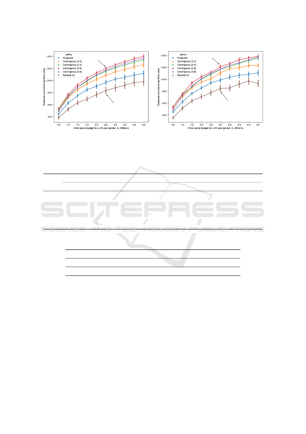
trials are depicted in Figure 2a and the 95% CIs are
listed in Table 1.
The results demonstrate that all policies outper-
form the benchmark Ranked list policy, and the Con-
tingency fund (θ = 0.6) policy performs the best
across all initial budgets studied. While the Contin-
gency fund policy with θ = 0.8 performed similar to
same policy with θ = 0.6, the latter consistently out-
performed the former as listed in Table 2. However,
it is worth noting that as the initial yearly budget in-
creases, the difference between the two policies be-
comes negligible.
The project selection results for each policy were
also examined to investigate why the Contingency
fund policies with higher reserves (θ = 0.6,θ = 0.8)
outperformed the other policies. It was noted that
these policies selected fewer high cost projects since
the available future budgets were limited by the re-
served funding. The total costs in the sample project
data ranged from 10s of millions to 10s of billions
of dollars. Therefore, the selection of a single high
cost project significantly reduces the number of lower
cost projects that can be selected in future years. Ad-
ditionally, the project values range less significantly
when compared to the total costs and are only mod-
erately correlated to the logarithm of the total cost.
As such, the selection of a high cost project does not
necessarily result in a significant increase in the cu-
mulative portfolio value. While all tested policies are
myopic and do not consider future effects, the Contin-
gency fund policy begins to mimic forward-looking
policies by forcing the reservation of funding for fu-
ture projects.
It may therefore be concluded that, for the sce-
nario and policies studied, using a knapsack-based
policy that reserves 60% of the available budget in
future years will provide the most value to defence.
While our scenario differs from that studied by Fisher
et al. (2015)—different project values, different cost
profiles, uncertainty in future budgets—our results
generally agree with their conclusion that holding
back budget results in a higher cumulative portfolio
value.
The aim of the second question is to evaluate the
impact that incorporating project cost uncertainty, of
delayed projects (Model-II), has on the policy recom-
Modelling Defence Planning as a Sequential Decision Problem
161

Ranked list
Contingnecy (0.6)
(a) Model-I.
Ranked list
Contingnecy (0.6)
(b) Model-II.
Figure 2: Expected cumulative portfolio value and 95% CI as a function of initial yearly budget for a 20-year period (B
0
) for
each decision policy described in subsection 4.3.
Table 1: Summary of 95% CIs for the percentage difference between each policy and the benchmark Ranked list policy when
using Model-I. Key: Rl = Ranked list, K = Knapsack, Cf (θ) = Contingency fund with a specific value of θ. All values are
rounded to two significant figures.
Policy Initial yearly budget for a 20-year period B
0
(Billions)
0.5 1.0 1.5 2.0 2.5 3.0 3.5 4.0 4.5 5.0
Rl - - - - - - - - - -
K [14, 30] [18, 31] [16, 28] [20, 30] [16, 28] [15, 25] [14, 25] [12, 21] [11, 19] [12, 23]
Cf (0.2) [27, 44] [35, 53] [31, 47] [35, 49] [32, 49] [29, 43] [28, 43] [27, 40] [25, 41] [27, 43]
Cf (0.4) [33, 51] [40, 60] [38, 53] [41, 56] [41, 59] [37, 55] [36, 52] [35, 50] [33, 50] [36, 54]
Cf (0.6) [38, 56] [45, 66] [44, 62] [48, 65] [46, 66] [42, 61] [41, 59] [40, 57] [39, 57] [41, 62]
Cf (0.8) [26, 44] [37, 58] [38, 55] [43, 59] [42, 62] [40, 58] [38, 56] [38, 54] [36, 54] [39, 59]
Table 2: Summary of 95% CIs for the percentage difference between the Contingency fund (θ = 0.6) policy and the Contin-
gency fund (θ = 0.8) policy when using Model-I. All values are rounded to one significant figure.
Initial yearly budget for a 20-year period B
0
(Billions)
0.5 1.0 1.5 2.0 2.5 3.0 3.5 4.0 4.5 5.0
[8, 10] [5, 7] [3, 5] [3, 5] [2, 4] [2, 4] [2, 3] [1, 3] [1, 3] [1, 3]
mendation. The results for the trials are depicted in
Figure 2b. Although a detailed analysis is not pre-
sented here, the results (similar to those in Figure 2a)
suggest that the Contingency fund (θ = 0.6) policy
outperforms the benchmark Ranked list policy across
all initial yearly budgets studied and performs better
than when other values of θ are used. The Model-II
results provide further evidence that for the scenario
and policies studied, the Contingency fund (θ = 0.6)
policy is robust with respect to different initial yearly
budgets, changes in future budgets, as well as changes
in costs of those projects there are delayed.
6 CONCLUSION
This paper presented initial work on the develop-
ment of a sequential decision model of the DND/CAF
multi-gate PAP. The objective was to investigate the
impact of different decision policies in a sequential
decision model that explicitly includes uncertainties
in budgets and the project information in each new
epoch.
The results from Model-I support the conclusion
that a Contingency fund policy that reserves 60% of
the available budget for future years performs the
best. A policy that reserves 80% of the available bud-
ICORES 2025 - 14th International Conference on Operations Research and Enterprise Systems
162

get performs almost as well when the initial yearly
budgets are large. Regardless, the Contingency fund
policies outperform both the benchmark Ranked list
policy and Knapsack policy. Model-II demonstrates
that the same decision policy, the Contingency fund
policy that reserves 60%, remains robust to cost un-
certainty in delayed projects and continues to outper-
form the other tested policies.
This initial model demonstrates the potential of a
sequential decision model to determine better deci-
sion policies for defence planning. Three areas of fu-
ture development have been identified. The first area
covers improvements to the sequential model to bet-
ter reflect the real-world dynamics of the DND/CAF
PAP. The initial model only covered the first step
of the PAP, therefore the model can be expanded
to cover the multiple gates of the PAP. Addition-
ally, the awarding of the value can be delayed to
when the project is delivered, rather than when the
project is selected. The modelled uncertainties can
also be expanded to capture changes in project value
and scheduling over time, as well as uncertainties that
may force the selection or cancellation of a project.
The second area of development covers the deci-
sion policies. The set of policies can be expanded
to include future-looking policies, and reinforcement
learning can be explored as a method for determining
an optimal decision policy. The last area of develop-
ment aims to improve the project dataset. The current
dataset is limited to a single year of projects. This
dataset can be expanded to include additional years
of historical data. Tools, such as natural language
processing, can be explored for extracting data from
historical project documentation. Data augmentation
techniques can also be explored for supplementing the
real project dataset.
The results presented here are encouraging, and
the completion of this investigation should pro-
vide more information to guide the management of
projects under uncertainty in defence planning.
ACKNOWLEDGMENTS
The authors would like to acknowledge the con-
tributions of Ammar Lakdawala, who implemented
an initial version of the sequential decision mod-
els in Python and conducted extensive testing in
spring 2024.
ACRONYMS
CAF Canadian Armed Forces
CI Confidence Interval
CIPPR Capital Investment Program Plan Review
CFA Cost Function Approximation
CFD Chief of Force Development
DND Department of National Defence
DP Dynamic Programming
MDP Markov Decision Process
NATO North Atlantic Treaty Organization
PAP Project Approval Process
PFA Policy Function Approximation
SPARC Strategic Portfolio Analyzer with Re-
configurable Components
VCDS Vice Chief of Defence Staff
VIPOR Visual Investment Optimization and Revi-
sion
REFERENCES
Balkaran, R. R. (2021). Process alignment: An assess-
ment of dnd project approval process in the 2019
project approval directive. Master’s thesis, Canadian
Forces College, Toronto, Ontario. Retrieved from:
https://www.cfc.forces.gc.ca/259/ 290/23/286/Balka-
ran.pdf.
Bellman, R. (1957). Dynamic Programming. Princeton
University Press.
Bertsekas, D. and Tsitsiklis, J. (1996). Neuro-Dynamic
Programming. Athena Scientific, Belmont, Mas-
sachusetts, First edition.
Brown, G. G., Dell, R. F., and Newman, A. M. (2004).
Optimizing military capital planning. Interfaces,
34(6):415–425.
Chen, C. and Wheaton, K. (2024). Investigating the Im-
pact of Project Dependencies on Capital Investment
Decisions in Defence. In 17th NATO Operations Re-
search and Analysis (OR&A) Meeting Proceedings.
NATO Science and Technology Organization. STO-
MP-SAS-OCS-ORA-2023.
Crawford, J., Do, J., Leduc, C., Malik, A., Gormley, K.,
Luebke, E., and Scherer, W. (2003). SWORD: the lat-
est weapon in the project selection arsenal. In IEEE
Systems and Information Engineering Design Sympo-
sium, 2003, pages 95–100.
Filinkov, A. and Dortmans, P. J. (2014). An enterprise port-
folio approach for defence capability planning. De-
fense & Security Analysis, 30(1):76–82.
Modelling Defence Planning as a Sequential Decision Problem
163

Fisher, B., Brimberg, J., and Hurley, W. (2015). An ap-
proximate dynamic programming heuristic to support
non-strategic project selection for the Royal Canadian
Navy. The Journal of Defense Modeling and Simula-
tion, 12(2):83–90.
Government of Canada (2019). Defence Investment
Plan 2018. Retrieved 22 October, 2024, from
https://www.canada.ca/en/ department-national-
defence/corporate/reports-publications/defence-
investment-plan-2018.html.
Government of Canada (2022). Status re-
port on transformational and major crown
projects. Retrieved 23 October, 2024 from
https://www.canada.ca/en/department-national-
defence/corporate/reports-publications/departmental-
plans/departmental-plan-2022-23/supplementary-
information/report-crown-project1.html#toc14.
Government of Canada (2024a). Our North, Strong
and Free: A Renewed Vision for Canada’s
Defence. Retrieved 15 October, 2024, from
https://www.canada.ca/en/ department-national-
defence/corporate/reports-publications/north-strong-
free-2024.html.
Government of Canada (2024b). Vice Chief of the Defence
Staff (VCDS). Retrieved 22 October, 2024, from
https://www.canada.ca/en/ department-national-
defence/corporate/organizational-structure/vice-
chief-defence-staff.html.
Harrison, K. R., Elsayed, S., Garanovich, I., Weir, T., Galis-
ter, M., Boswell, S., Taylor, R., and Sarker, R. (2020).
Portfolio optimization for defence applications. IEEE
Access, 8:60152–60178.
Kuo, F. and Sloan, I. (2005). Lifting the curse of
dimensionality. Notices of the American Mathemat-
ical Society, 52(11):1320–1328. Retrieved from:
https://www.ams.org/journals/notices/200511/ fea-
sloan.pdf?adat=December%202005&trk=200511fea-
sloan&cat=feature&galt=feature.
Locatelli, A. (2023). Optimization methods for knapsack
and tool switching problems. 4OR, 21:715–716.
Moallemi, E. A., Elsawah, S., Turan, H. H., and Ryan, M. J.
(2018). Multi-objective decision making in multi-
period acquisition planning under deep uncertainty.
In 2018 Winter Simulation Conference (WSC), pages
1334–1345.
North Atlantic Treaty Organization (2022). NATO
2022 Strategic Concept. Retrieved 23 Octo-
ber, 2024, from https://www.act.nato.int/wp-content/
uploads/2023/05/290622-strategic-concept.pdf.
North Atlantic Treaty Organization (2024). Washing-
ton Summit Declaration. Retrieved 23 October,
2024, from https://www.nato.int/cps/en/natohq/ offi-
cial texts 227678.htm.
Office of the Parliamentary Budget Officer (2021). The cost
of Canada’s surface combatants: 2021 update and
options analysis. Retrieved 22 October, 2024, from
https://www.pbo-dpb.ca/en/publications/RP-2021-
040-C–cost-canada-surface-combatants-2021-update-
options-analysis–cout-navires-combat-canadiens-
mise-jour-2021-analyse-options.
Powell, W. (2011). Approximate dynamic programming:
Solving the curses of dimensionality. Wiley, Hoboken,
New Jersey, Second edition.
Powell, W. (2022). Reinforcement learning and stochastic
optimization: A unified framework for sequential de-
cisions. Wiley, Hoboken, New Jersey.
Puterman, M. (2005). Markov Decision Processes: Discrete
stochastic dynamic programming. Wiley, Hoboken,
New Jersey.
Rempel, M. and Young, C. (2017). VIPOR: A visual analyt-
ics decision support tool for capital investment plan-
ning. Scientific Report DRDC-RDDC-2017-R129,
Defence Research and Development Canada.
Roncolato, G. (2022). The character of war is
constantly changing: Organizations and peo-
ple who can rapidly and effectively adapt are
more likely to prevail. U.S. Naval Institute
Proceedings, 148/5/1.431. Retrieved from:
https://www.usni.org/magazines/proceedings/2022/may
/character-war-constantly-changing.
Rossignol, M. (1998). Replacement of shipborne and
rescue helicopters. Retrieved 23 October, 2024,
from https://www.publications.gc.ca/Collection-
R/LoPBdP/CIR/943-e.htm.
Salo, A., Doumpos, M., Liesi
¨
o, J., and Zopounidis, C.
(2024). Fifty years of portfolio optimization. Euro-
pean Journal of Operational Research, 318(1):1–18.
Shafi, K., Elsayed, S., Sarker, R., and Ryan, M. (2017).
Scenario-based multi-period program optimization for
capability-based planning using evolutionary algo-
rithms. Applied Soft Computing, 56:717–729.
Tsaganea, D. (2005). Appropriation of funds for anti-
ballistic missile defence: a dynamic model. Kyber-
netes, 34(6):824–833.
U.S. Government Accountability Office (2020). Cost esti-
mating and assessment guide: Best practices for de-
veloping and managing program costs. Technical Re-
port GAO-20-195G, U.S. Government Accountability
Office.
ICORES 2025 - 14th International Conference on Operations Research and Enterprise Systems
164