Attached Shadow Constrained Shape from Polarization

Momoka Yoshida

, Ryo Kawahara

2 a

and Takahiro Okabe

3 b

Department of Artiﬁcial Intelligence, Kyushu Institute of Technology, 680-4 Kawazu, Iizuka, Fukuoka 820-8502, Japan

Graduate School of Informatics, Kyoto University, Yoshida-honmachi, Sakyo-ku, Kyoto, 606-8501, Japan

Information Technology Track, Faculty of Engineering, Okayama University,

3-1-1 Tsushima-naka, Kita-ku, Okayama 700-8530, Japan

Keywords:

3D Shape Reconstruction, Polarization, Shape-from-X.

Abstract:

This paper tackles a long-standing challenge in computer vision: single-shot, per-pixel surface normal recov-

ery. Although polarization provides a crucial clue to solving this problem, it leaves ambiguity in the normal

estimation even when the refractive index is known. Therefore, previous studies require additional clues or

assumptions. In this paper, we propose a novel approach to resolve this ambiguity and the unknown refrac-

tive index simultaneously. Our key idea is to leverage attached shadows to resolve normal ambiguity while

measuring the refractive index based on wavelength characteristics in a single-shot scenario. We achieve this

by separating the contributions of three appropriately placed narrow-band light sources in the RGB channel.

We further introduce disambiguation uncertainty to address cast shadows and achieve more accurate normal

recovery. Our experimental evaluations with synthetic and real images conﬁrm the effectiveness of our method

both qualitatively and quantitatively.

1 INTRODUCTION

Reconstructing dense 3D surfaces has been a central

research topic in computer vision. Single-shot re-

covery of the surface normals, in particular, has vari-

ous applications, including industrial product inspec-

tion, robotics, digital archiving, and medicine. On

the other hand, as an independent problem of depth

sensing, solving per-pixel surface normals from a sin-

gle 2D image is a long-standing, challenging task for

ﬁne-detailed geometry.

Polarization is one of the crucial cues for surface

shape recovery. When a surface reﬂects unpolarized

light, the reﬂected light becomes partially polarized

depending on the surface normal and refractive in-

dex. The shape recovery method utilizing this cue

is called Shape from Polarization (SfP). However, the

core issue is the ambiguity that exists in its normal es-

timation, even with a known refraction index. There-

fore, previous SfP methods require additional cues or

assumptions for per-pixel estimation, such as known

albedo for shading cues and surface integrability.

Are any additional pixel-independent cues avail-

able for a per-pixel solution in a single-shot scenario

https://orcid.org/0000-0002-9819-3634

https://orcid.org/0000-0002-2183-7112

for objects with various shapes and textures? The dis-

ambiguation of the normal solution by fusion with a

depth or low-frequency geometry cannot be entirely

separated from the issue of shape discontinuities. We

tackle obtaining a unique solution for the normals in

this single-shot problem while relaxing the need for

assumptions about the object.

In this paper, we show that we can identify the

correct answer of SfP solution candidates by the at-

tached shadows. Our focus for achieving this concept

in a single-shot scenario is to leverage three differ-

ent narrow bandwidth light sources that are separa-

ble by RGB channels in a direction layout that dis-

ambiguates the SfP. We further show that the refrac-

tive index, which is often uniform across the object

surface, can be estimated from the consistency of the

zenith angle at each of the three wavelengths and ap-

plied to unknown dielectric materials.

In addition, to distinguish cast shadows and elim-

inate ambiguous estimations, we introduce certainty

based on a fusion of attached shadow clarity metrics

and strategies for detecting cast shadows. We apply

the belief propagation method for regions of low cer-

tainty to select a normal candidate and recover the en-

tire shape.

We experimentally validate our method on ob-

jects with various shapes, materials, and textures. We

640

Yoshida, M., Kawahara, R. and Okabe, T.

Attached Shadow Constrained Shape from Polarization.

DOI: 10.5220/0013248700003912

Paper published under CC license (CC BY-NC-ND 4.0)

In Proceedings of the 20th International Joint Conference on Computer Vision, Imaging and Computer Graphics Theory and Applications (VISIGRAPP 2025) - Volume 3: VISAPP, pages

640-647

ISBN: 978-989-758-728-3; ISSN: 2184-4321

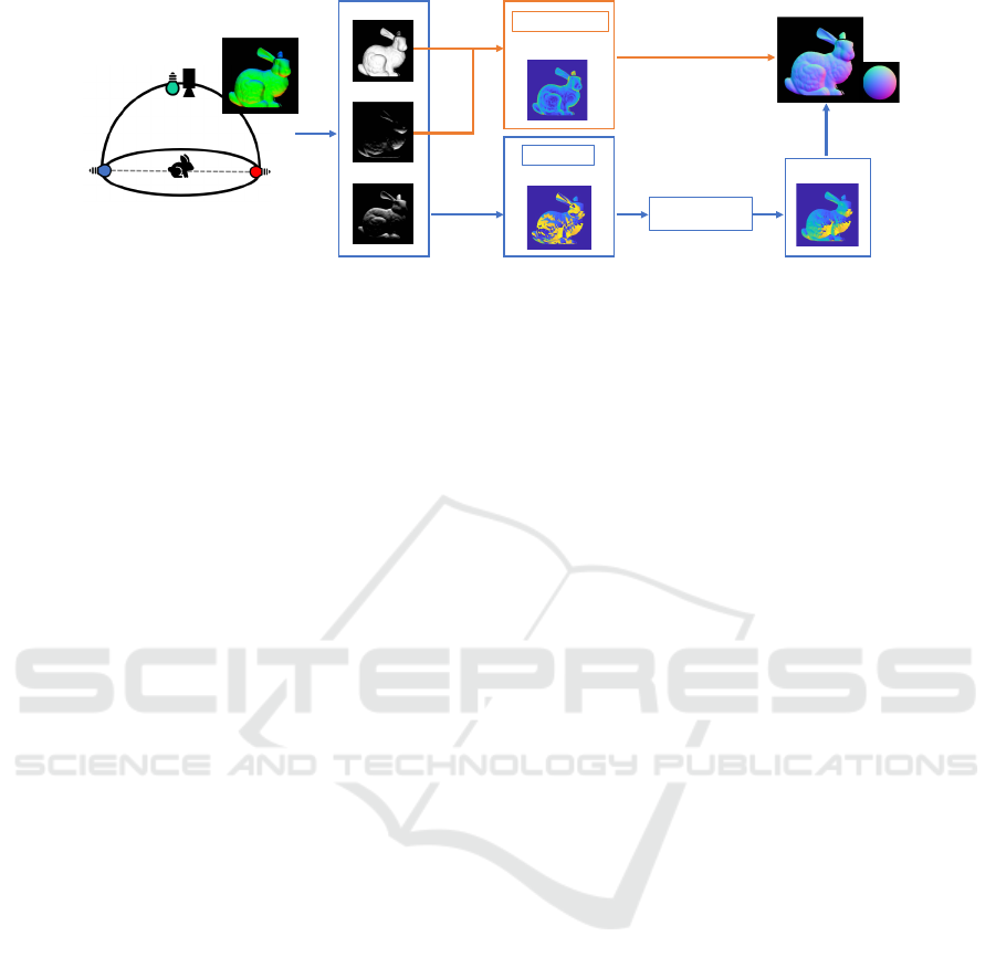
Input

Output

Refractive index

Zenith angle

Azimuth angle

Uncertainty-aware

disambiguation

Certainty

Azimuth angle

(a)

(b)

(c)

Figure 1: Attached Shadow Constrained Shape from Polarization. (a) We utilize single-shot images taken under three appro-

priately placed narrow-band light sources. (b) By separating and utilizing their wavelength contributions in the RGB channel,

we achieve normal disambiguation through attached shadows while estimating the object’s refractive index. This stage also

provides certainty for pixels where ambiguity becomes unstable due to cast shadows or shadow boundaries. (c) We apply

belief propagation to this low-certainty region and achieve per-pixel normal recovery in a single shot.

conducted a thorough quantitative evaluation of the

proposed method’s impact on ”shadow-based disam-

biguation,” ”cast shadow handling with the introduc-

tion of disambiguation certainty,” and ”refractive in-

dex estimation” using synthetic images. Additionally,

we demonstrated these effects qualitatively through

real image experiments.

Our main contributions are as follows,

• Demonstrating attached shadows can be used to

identify the correct normals among SfP solution

candidates.

• Achieving disambiguation in a single shot by sep-

arating and utilizing the contributions of three

different narrow-band light sources in the RGB

channel.

• Introducing a novel method for estimating the re-

fractive index of an object’s surface from the con-

sistency of the zenith angle at three wavelengths.

• Deﬁning the certainty of disambiguation and ap-

plying the belief propagation method to uncertain

regions to improve the accuracy of shape recon-

struction.

2 RELATED WORK

Methods for normal estimation have advanced with

many challenges and solutions. Physics-based deduc-

tive methods such as photometric stereo (Woodham,

1980; Ackermann et al., 2015), shape from shading

(Ikeuchi and Horn, 1981; Zhang et al., 1999), and SfP

(Atkinson and Hancock, 2006; Miyazaki et al., 2003;

Rahmann and Canterakis, 2001) have been proposed

for decades. However, single-shot normal estimation

has always been a challenging task as an inverse prob-

lem from 2D to 3D.

Multi-spectral photometric stereo (MPS) (Ander-

son et al., 2011; Chakrabarti and Sunkavalli, 2016;

Ozawa et al., 2018; Guo et al., 2021) is one approach

to this challenge. MPS utilizes light sources of differ-

ent wavelengths to estimate normals from single-shot

images. However, since the intensity observed by the

camera depends on the object’s reﬂectance, additional

constraints are required, such as albedo, chromaticity

clustering, and integrability of the surface geometry.

Thus, a barrier to per-pixel single-shot estimation ex-

ists.

On the other hand, the single-shot SfP method

has the problem that the zenith angle depends on the

refractive index, so the wrong refractive index dis-

torts the normal (Kadambi et al., 2015). Addition-

ally, it is known that there are two candidate solu-

tions for the azimuth angle (Atkinson and Hancock,

2006; Miyazaki et al., 2003). Therefore, single-shot

SfP also requires additional constraints or prior, such

as shading cues and surface integrability (Mahmoud

et al., 2012; Smith et al., 2016; Smith et al., 2018).

There are methods for polarization and multi-spectral

fusion. Huynh et al. (Thanh et al., 2015) proposed a

method for simultaneously estimating the normal and

refractive index using a polarization multi-spectral

image. However, this method assumes that the scene

geometry is smooth and convex.

In contrast, we leverage the binary information of

whether each pixel is an attached shadow or not to

resolve the ambiguity of SfP. Utilizing the fact that

the normal solution space is limited by the bound-

ary of the attached shadow(Kriegman and Belhumeur,

2001), our method eliminates assumptions about the

chromaticity of the object and the integrability of

its shape, allowing independent estimation for each

pixel. Therefore, our method realizes a more ﬂexible

single-shot normal estimation, even for textured ob-

jects.

Attached Shadow Constrained Shape from Polarization

641

Zenith angle

Azimuth angle

Surface

normal

Surface

normal

Figure 2: Ambiguity of surface normals in Shape from Po-

larization. Since π-ambiguity exists in the azimuth angle

estimated from the diffuse polarization, there are two can-

didates for the normal.

Recently, polarization-based methods using deep

prior (Ba et al., 2020; Deschaintre et al., 2021; Hwang

et al., 2022; Lei et al., 2022) have shown effective re-

sults, but they rely on supervised learning and require

large data sets. In contrast, our method achieves nor-

mal recovery from a single input image and estimates

objects’ refractive indices.

3 BASICS: SHAPE FROM

POLARIZATION

We will ﬁrst brieﬂy introduce the fundamental theory

of SfP and its ambiguity, which needs to be resolved.

3.1 Polarization

Unpolarized light consists of electromagnetic waves

oscillating in a random direction and having uniform

intensity around the direction of light travel. Sunlight

and common light sources correspond to this type of

light. When an object reﬂects unpolarized light, the

oscillation direction of the electromagnetic wave is

biased, resulting in partially polarized light. Polar-

ization cameras can extract angular components by

observing light through a linear polarizer at a certain

angle. When rotating the linear polarizer with angle

ψ, the intensity of light can be described as following

sinusoidal:

I(ψ) = I

max

cos

(ψ −ϕ) + I

min

sin

(ψ −ϕ)

max

+ I

min

max

−I

min

cos2(ψ −ϕ),

(1)

where I

max

and I

min

are the maximum and minimum

intensity for angle ψ. The angle ϕ is called the an-

gle of linear polarization (AoLP), where observed in-

tensity reaches I

max

. Thanks to recent advances in

technology, quad-bayer polarization cameras can pro-

vide polarization images for four ﬁlter angles ψ =

(0,π/4,π/2,3π/4) from a single image. Hence, we

can recover the sinusoidal in single-shot (Huynh et al.,

2010).

3.2 Normal Estimation from

Polarization and Its Ambiguity

The basic concept of SfP is to utilize the fact that the

polarization changes during reﬂection depending on

the surface normal, and to calculate the surface nor-

mal as an inverse problem. Fresnel equations can de-

scribe these relationships, which differ for diffuse and

specular reﬂection. In this study, we mainly focus on

the polarization of diffuse reﬂections, as we utilize a

distant point source. The treatment of specular reﬂec-

tions will be discussed in Sec. 4.

As shown in Fig. 2, let us denote the surface nor-

mal n by the zenith angle θ and azimuth angle φ fol-

lows,

n =





sinθ cos φ

sinθ sin φ

cosθ





. (2)

Since the diffuse polarization component has a max-

imum intensity in the direction along the plane

spanned by the viewing direction (z-axis in the Fig. 2)

and the normal, the following holds;

φ = ψ or ψ + π. (3)

On the other hand, independent of this, the zenith

angle θ depends on the Fresnel transmission ratio r

min

max

, and the following holds (Huynh et al., 2010);

θ ≃ arcsin

√

1 −r

−2rη + 1

. (4)

Thus, even when the refractive index is known, there

are two candidate normals (n, ˆn) due to the ambigu-

ity of the azimuth angle in Eq. 3.

4 METHOD

We propose a physics-based, per-pixel solution for

single-shot SfP without assuming geometry integra-

bility or uniform albedo. We employ a quad-Bayer

color polarization camera and capture objects simul-

taneously illuminated by three light sources of differ-

ent directions and colors as shown in Fig. 1(a).

For a perspective projection camera, it can be deﬁned

similarly as a local coordinate system such that the viewing

direction becomes the z-axis (Pistellato and Bergamasco,

2024).

VISAPP 2025 - 20th International Conference on Computer Vision Theory and Applications

642

Assumptions. Our method relies on several as-

sumptions throughout the paper:

1. Orthographic camera or known focal length

2. Dielectric objects

3. Diffuse-dominant materials

4. Known narrow-band distant point sources

5. Spatially uniform refraction index

Note that assumption 3 requires that the amplitude

of the diffuse polarization component be larger than

the amplitude of the specular polarization component,

which does not signiﬁcantly limit the material (Smith

et al., 2018). Additionally, We typically observe spec-

ular reﬂections as saturated sharp highlights with our

three distant point sources setup. We exclude these

highlight regions from our estimation to maintain the

dynamic range. Consequently, the observations in the

target region can be approximated by diffuse polar-

ization components (Kadambi et al., 2015), and Eq. 4

holds.

4.1 Estimation of Candidate Normals

with Unknown Refraction Index

This section shows that we can estimate candidate

normals with unknown refractive indices under our

narrow-band wavelength source. Since the refractive

index depends on wavelength, we can use the fact that

different Fresnel transmittances in each RGB band

refer to the same zenith angle. When using a wide-

bandwidth light source, even if the spectral intensity

is known, note that the contribution of wavelengths

will not be uniform for objects with spatially varying

spectral reﬂectance. We can practically avoid this is-

sue with narrow bandwidth light sources.

Let η

, η

, and η

be the refractive indices, and

, r

, and r

be the observed Fresnel transmittance

ratio for each RGB wavelength, respectively, and the

following holds from Eq. 4,

1 −r

−2r

+ 1

1 −r

−2r

+ 1

1 −r

−2r

+ 1

1 −r

−2r

+ 1

(5)

Using two or more pixels with different zenith angles

can estimate the refractive indices of one band pair

(e.g. R and B). We further estimated the refractive in-

dices η

, η

using RANSAC for robust estima-

tion. The zenith angle is then estimated using the re-

fractive indices and Fresnel transmission coefﬁcients.

(a) Acute angle or obtuse angle

(b) Both acute angle

Figure 3: Overview of disambiguation. The condition un-

der which the normal (orange arrow) can be disambiguated

by whether it is an attached shadow or not is whether its

status changes depending on the candidate normals. i.e.,

when the angle between the normal and the light source is

divided into (a) an acute angle and an obtuse angle, it can

be resolved, while it cannot in the case of (b).

The azimuth angle is estimated from Eq. 3. Up

to this point, we obtain two potential normals for the

object with an unknown refractive index.

4.2 Azimuthal Disambiguation from

Attached Shadow

4.2.1 Overview of Disambiguition

We resolve that azimuth angle ambiguity based on

the attached shadow. The clue, whether the attached

shadow or not, suggests the angle between the direc-

tion of the light source and the true normal. That is,

the observed intensity depends on the inner product

of the source direction and the true normal, which

is positive when the pixel is illuminated. Also, the

inner product at the attached shadow pixels is neg-

ative. Therefore, by taking the inner product of the

source direction and the candidate normals and select-

ing the candidate normals that are consistent with the

observed radiance, the π-ambiguity regarding the nor-

mal azimuth angle can be resolved.

Let us consider the example shown in Fig. 3 for

a better understanding of the conditions required for

disambiguation. In Fig. 3(a), the angle between the

light source direction and the candidate normal is

acute on one side and obtuse on the other, allowing

us to resolve the ambiguity. However, both angles are

acute in Fig. 3(b), so the ambiguity cannot be resolved

for that pixel.

4.2.2 Design of Light Source Direction

All pixels need to be illuminated to obtain candidate

normals by polarization analysis. Considering ob-

jects with various shapes, our reasonable approach is

to illuminate one of the light sources coaxially with

the viewing direction (we call it base light hereafter).

Therefore, this section discusses the design of the re-

Attached Shadow Constrained Shape from Polarization

643

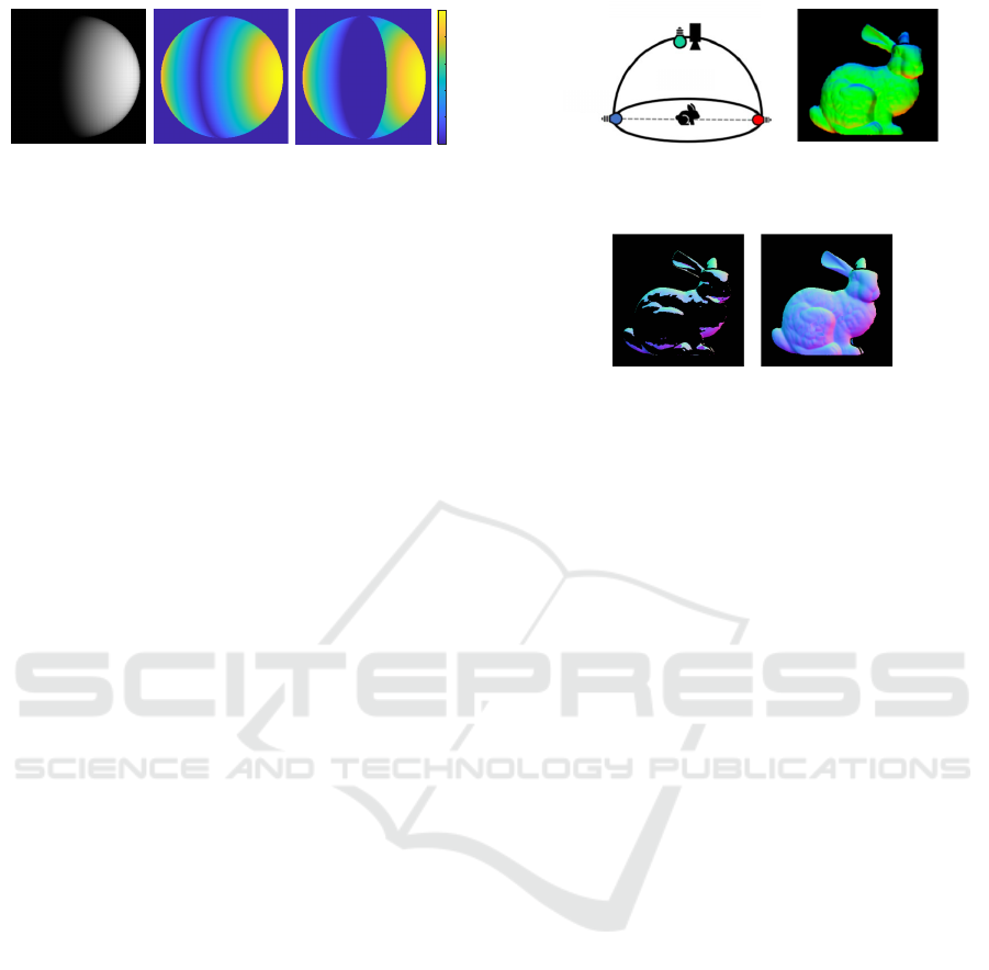
(a) Input (b) | cosα | (c) Certainty

0.1

0.2

0.3

0.4

0.5

0.6

0.7

0.8

0.9

0.1

0.2

0.3

0.4

0.5

0.6

0.7

0.8

0.9

1.0

0.8

0.6

0.4

0.2

Figure 4: Certainty of disambiguation. (a) (b) Near the

boundary of the attached shadow, it is ambiguous whether it

is a shadow or not. (c) Furthermore, disambiguation is not

feasible in the case corresponding to Fig. 3(b), so we deﬁne

certainty as a combination of these two.

maining two source directions to disambiguate the

normals.

The discussion in Sec. 4.2.1 indicates that when

there is only a single side light source, it should be

illuminated from a direction orthogonal to the base

light source, but when there are two side light sources,

the optimal arrangement is non-trivial. Therefore,

we consider a practical layout by introducing the cer-

tainty of disambiguation.

Certainty of Disambiguation. Near the boundary

of the attached shadow, where the inner product of

the normal and light source direction is zero, shadow

or not is ambiguous and difﬁcult to determine. There-

fore, we introduce a certainty of disambiguation s

minimize the number of ambiguous pixels.

Basically, the certainty of either attached shadow

or not can be measured by the absolute value of the

inner product of the light source direction and the nor-

mal. Thus, we deﬁne the certainty of disambiguation

for a side light source as follows,

(

|cos α| (cosα

cosα < 0),

0 otherwise,

(6)

where cos α and

cosα denote the inner products of a

light source and two candidate normals, respectively.

Fig. 4 shows an example of this certainty. A pixel that

satisﬁes cosα

cosα < 0 (the case of Fig. 3(b)) has zero

certainty because the ambiguity cannot be resolved.

For extensions on multiple side light sources, we

can focus on the fact that disambiguation is to be

achieved by one of them. Therefore, suppose that the

base light source corresponds to the G channel; the

certainty with the two side light sources can be de-

scribed using the individual certainties s

p,R

and s

p,B

as follows,

= max{s

p,R

p,B

}. (7)

As a simulation experiment, we conducted a grid

search with 1-degree intervals to ﬁnd the optimal

direction of the two-side light sources that maxi-

mizes the certainty calculated by Eq. 7 for a refer-

ence sphere. Our ﬁndings suggest that the position

Lights

Color polarization camera

Object

(a)

(b)

Figure 5: Our light source conﬁguration. (a) Overview. (b)

An example of the captured image.

(a) (b)

Figure 6: Uncertainty-aware Azimuthal Disambiguation.

(a) We detect cast shadows and ambiguous attached shad-

ows by our proposed certainty and (b) disambiguate nor-

mals by belief propagation.

where the three light sources are orthogonal to each

other is suitable. Furthermore, as discussed in the next

section, we extend this model to consider cast shad-

ows and determine the practical arrangement of light

sources.

Cast Shadow Handling. Cast shadows are another

factor that must be considered when designing the di-

rection of the light source. It is essential to ﬁnd the

cast shadow since the method in Sec. 4.2.1 cannot be

applied to resolve the ambiguity. However, since both

attached and cast shadows are not illuminated, it is

impossible to identify which shadow is which by the

observed luminance.

Based on these results and insights, as shown in

Fig. 5, we place the two side light sources (R and B)

so that they are orthogonal to the base light source

(G) and opposite each other. When either light source

does not illuminate the pixels, they are in a cast

shadow from at least one of the light sources. The

disambiguation based on the attached shadow cannot

be applied to such pixels. Thus, we extend the cer-

tainty for these pixels as the region where s

= 0, and

we utilize the method described in the next section to

resolve the ambiguity.

4.3 Uncertainty-Aware Azimuthal

Disambiguation

In this section, we propose a method for selecting can-

didate normals by propagating adjacent high-certainty

azimuths for pixels with cast shadows or small cer-

tainty. We solve this as a graph optimization problem

with each pixel as a node.

VISAPP 2025 - 20th International Conference on Computer Vision Theory and Applications

644

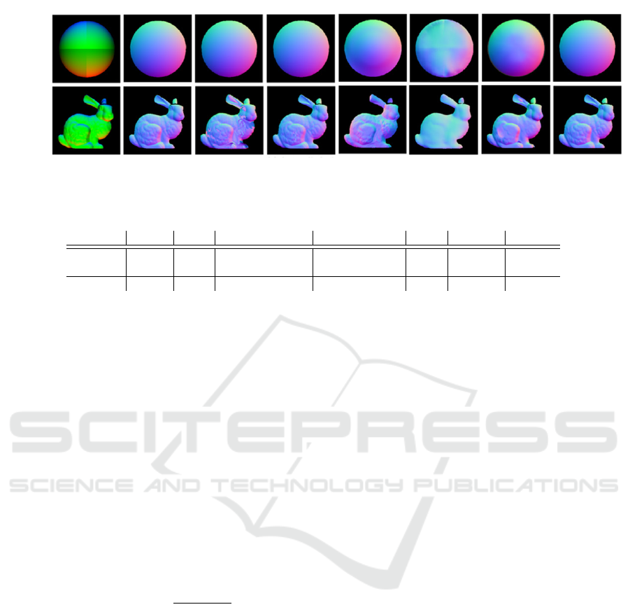
Sphere

(Textured)

Bunny

Input

Ours

DfP

DeepSfP

DeepPol

w/o certainty

w/o η estimation

Figure 7: The reconstruction results with synthetic data. The leftmost is input single-shot images. The color of the results is

shown based on the normal XYZ component.

Table 1: Quantitative evaluation of recovered normals. (Mean angular errors in degree).

Input Object Ours w/o C.S. handling w/o η estimation DfP DeepSfP DeepPol

Synthetic

Sphere 0.03 0.03 2.01 8.17 30.77 11.84

Bunny 0.20 12.25 2.13 15.75 33.56 14.74

Real Sphere 6.44 22.95 6.48 22.92 35.89 12.89

In particular, assuming the azimuth angle of each

pixel φ

takes two states, ψ or ψ+ π, consider the fol-

lowing energy cost function w.r.t. the set of azimuth

angles Φ of all pixels;

E(Φ) =

∑

p∈P

∑

q∈N

(p,φ

,φ

) +

∑

p∈P

(p,φ

), (8)

where P denotes the set of all pixels, and N

denotes

the set of pixels q in the four neighbors to pixel p.

represents the data cost term, which is set to a

uniform value regardless of the state when the cer-

tainty s

is s

< γ for some threshold γ. C

repre-

sents the smoothness cost term formulated by the dis-

similarity of azimuth angles between adjacent pixels.

The smoothness cost term C

can be described us-

ing the vector representation of azimuthal directions

= (cosφ

,sin φ

)

⊤

and v

= (cosφ

,sin φ

)

⊤

(p,φ

,φ

) = 1 −

·v

+ 1

. (9)

We minimize the energy function in Eq. 8 with be-

lief propagation. Speciﬁcally, we input the energy

E(Φ) into the potential function and compute Φ to

maximize it. The potentials for C

and C

, respec-

tively, become as follows,

(p,φ

) = e

−C

(p,φ

)

(p, φ

,φ

) = e

−C

(p,φ

,φ

)

(10)

Therefore, using the following message function, Φ

can be obtained by iteratively propagating belief to

adjacent pixels until convergence,

p→q

(φ

) =

∑

={η,η+π}

(p, φ

) ×B

(p, φ

,φ

)

∏

k∈N

k→q

(φ

,φ

(11)

Since only the message m

p→q

is updated and B

, B

are ﬁxed, it converges to a quasi-globally optimal so-

lution.

Fig. 6 show an example of our disambiguation.

In regions with cast shadows or low certainty s

(black area in “Bunny”), our BP effectively resolves

ambiguity, enabling us to select a candidate normal

uniquely.

5 EXPERIMENTAL RESULT

We experimentally evaluate the effectiveness of our

method using synthetic and real images. Based on the

discussion in Sec. 4.2.2, our setup consists of the base

light source illuminated from the viewing direction

for the candidate normals estimation and two light

sources illuminated from the side direction for the az-

imuth angle disambiguation.

As for disambiguation based on attached shadows,

to avoid uncertain detection of illuminated pixels, the

certainty threshold is empirically set to γ = 0.4 for

all the data, and for the cast shadow pixels and low-

certainty pixels, disambiguation is performed using

the method described in Sec. 4.3.

As a baseline for comparison, we used the

physics-based (Smith et al., 2016), learning-based

(Ba et al., 2020)(Deschaintre et al., 2021), our method

without cast shadow handling (”w/o certainty”) and

our method without refractive index estimation (”w/o

η estimation”). For the methods (Smith et al., 2016)

and (”w/o η estimation”), the normal is estimated by

assuming that the refractive index of the base light

source is 1.5, following previous works.

Attached Shadow Constrained Shape from Polarization

645

5.1 Quantitative Evaluation with

Synthetic Data

We quantitatively evaluate the reconstruction accu-

racy of our method using synthetic images. As shown

in Fig. 5, we correspond the base light source to the

G-channel for the proof of concept. We used ren-

dered objects with different shapes (“Sphere” and

“Bunny”) which have ideal diffuse reﬂective surfaces.

We added texture to the “Sphere” to represent the

spatially varying albedo. The refractive index was set

to (R:1.44, G:1.45, B:1.46) for all the objects.

Fig. 7 and Table 1 show the results of surface nor-

mal recovery. These results clearly demonstrate that

the proposed method can recover the shape of objects

with bumps, such as “Bunny,” with higher accuracy

than the baseline results. In addition, the shape is suc-

cessfully recovered without any assumptions regard-

ing texture or albedo, as in the results for the texture-

added “Sphere.”

5.2 Real World Objects

We also conduct evaluation experiments using real

images to demonstrate the effectiveness of our

method qualitatively. We use narrow-band LED light

sources of 450 nm, 525 nm, and 640 nm as unpo-

larized light sources. We capture the image using a

quad-Bayer color polarization camera (Blackﬂy BFS-

U3-51S5P-C). We built a single-shot system in our

indoor environment to demonstrate the proof of con-

cept. The position of the light source was adjusted in

advance using a reference sphere different from the

one used for the evaluation. The objects we use have

different shapes, textures, and materials (“Sphere,”

“Pear,” “Elephant”).

Fig. 8 shows the results of the surface normal es-

timation. Note that our method does not account for

specular reﬂection, so the areas of specular reﬂection

in the input image are masked out for evaluation. The

results clearly show that our method can successfully

recover the normals of these objects, regardless of the

textures and complex surface geometry. In order to

quantitatively evaluate the shape recovery results of

real objects, we obtain the ground truth of the normal

using a sphere with a known diameter (“Sphere”). Ta-

ble 1, the bottom row shows the result of our method

has the best performance for the surface recovery.

5.3 Ablation Study

The effectiveness of introducing certainty and ad-

dressing cast shadows by BP is demonstrated by the

method (”w/o certainty”). As Figs 7,8 show, quali-

Table 2: Results of refractive index estimation.

Input Object Ours GT

Synthetic

Sphere 1.45 1.45

Bunny 1.45 1.45

Real

Sphere 1.51 –

Pear 1.44 –

Elephant 1.41 –

tative differences are clearly evident in the concave

areas where cast shadows occur and in the boundary

areas and attached shadows become ambiguous. Ta-

ble 1 also demonstrates the effect quantitatively.

Additionally, the method (”w/o η estimation”)

demonstrates the impact of refractive index estima-

tion on the estimation results. This appears to be a

distortion of the normal’s zenith angle, and its im-

provement is shown especially in Table 1. Most im-

portantly, this result shows that the proposed method

is applicable to objects with unknown refractive in-

dices.

5.4 Refractive Index Estimation

Table 2 shows the results of refractive index estima-

tion. We show the refractive indices of the base light

sources (the G channel in the synthetic image exper-

iment and the B channel in the real image experi-

ment) used for zenith angle estimation. The results

with synthetic images quantitatively show that the

proposed method is capable of highly accurate esti-

mation. Also, while ground truth is not available in

the results with real images, we ﬁnd they are within

the typical range of refractive indices for each mate-

rial.

6 CONCLUSION

This paper proposes a practical single-shot SfP that

estimates the per-pixel normal of objects with un-

known refractive indices. By effectively arranging

narrow-band R, G, and B light sources and a color po-

larization camera, we achieve effective disambigua-

tion by utilizing attached shadows and estimating the

unknown refractive indices, thus relaxing the conven-

tional single-shot SfP assumptions. Furthermore, we

introduce a novel BP-based uncertainty-aware disam-

biguation to address regions with cast shadows and

ambiguous presence or absence of attached shadows.

The major limitation of our method is that it assumes

diffuse-dominant surfaces. Even when leveraging a

distant point source, for some objects with high sur-

face roughness and specular reﬂectance, the specular

component will dominate in a wide area, limiting the

range of objects that can be recovered. Therefore, one

VISAPP 2025 - 20th International Conference on Computer Vision Theory and Applications

646

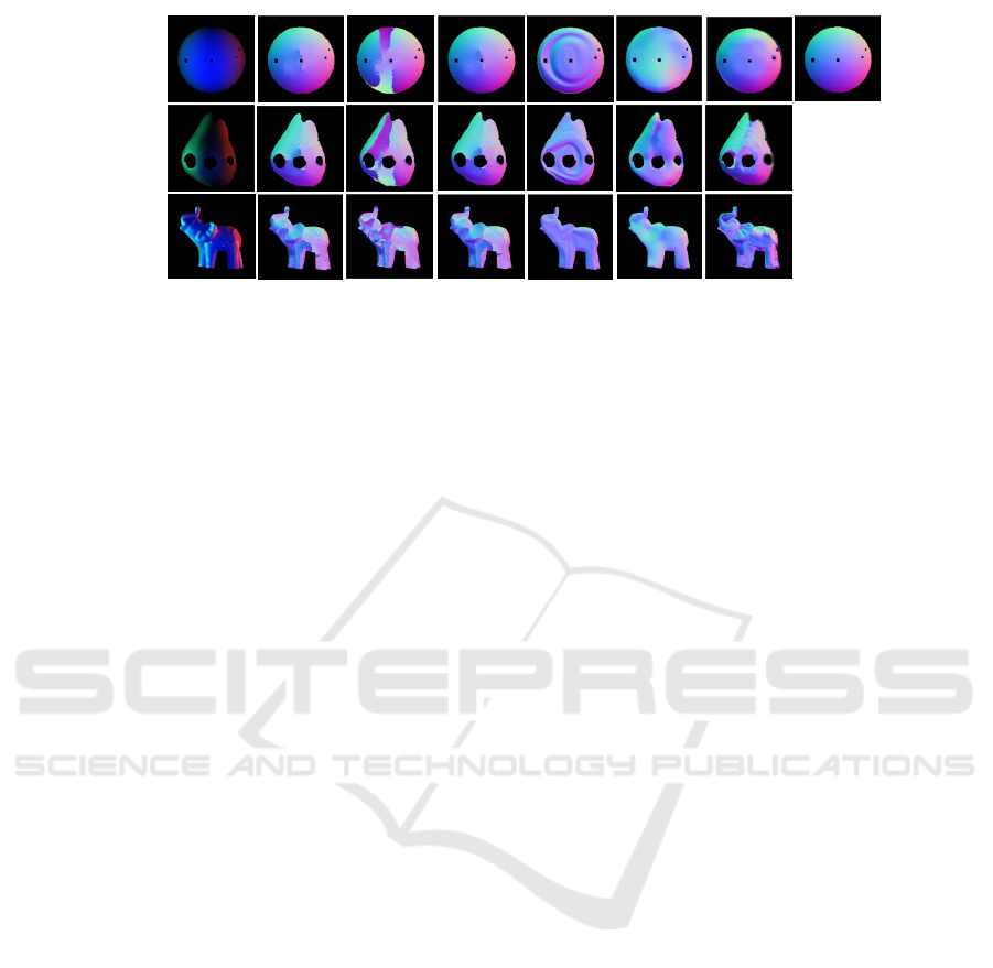
Sphere

Pear

Elephant

Input

Ours

DfP

DeepSfP

DeepPol

w/o certainty

w/o η estimation

Figure 8: The reconstruction results of real-world objects. The leftmost is input single-shot images. The color of the results

is shown based on the normal XYZ component.

future work is to extend our method to the specular-

dominant surfaces. Another limitation arises from

overly complex surfaces, which disrupt the azimuthal

similarity of neighboring pixels and create extensive

cast shadows.

ACKNOWLEDGEMENTS

This work was supported by JSPS KAKENHI Grant

Numbers JP20H00612 and JP22K17914.

REFERENCES

Ackermann, J., Goesele, M., et al. (2015). A survey of pho-

tometric stereo techniques. Foundations and Trends®

in Computer Graphics and Vision, 9(3-4):149–254.

Anderson, R., Stenger, B., and Cipolla, R. (2011). Color

photometric stereo for multicolored surfaces. In

ICCV, pages 2182–2189. IEEE.

Atkinson, G. A. and Hancock, E. R. (2006). Recovery of

surface orientation from diffuse polarization. IEEE

TIP, 15(6):1653–1664.

Ba, Y., Gilbert, A., Wang, F., Yang, J., Chen, R., Wang, Y.,

Yan, L., Shi, B., and Kadambi, A. (2020). Deep shape

from polarization. In ECCV, pages 554–571.

Chakrabarti, A. and Sunkavalli, K. (2016). Single-image

rgb photometric stereo with spatially-varying albedo.

In 3DV, pages 258–266. IEEE.

Deschaintre, V., Lin, Y., and Ghosh, A. (2021). Deep polar-

ization imaging for 3d shape and svbrdf acquisition.

In CVPR, pages 15567–15576.

Guo, H., Okura, F., Shi, B., Funatomi, T., Mukaigawa, Y.,

and Matsushita, Y. (2021). Multispectral photomet-

ric stereo for spatially-varying spectral reﬂectances: A

well posed problem? In CVPR, pages 963–971.

Huynh, C. P., Robles-Kelly, A., and Hancock, E. (2010).

Shape and refractive index recovery from single-view

polarisation images. In CVPR, pages 1229–1236.

Hwang, I., Jeon, D. S., Munoz, A., Gutierrez, D., Tong, X.,

and Kim, M. H. (2022). Sparse ellipsometry: portable

acquisition of polarimetric svbrdf and shape with un-

structured ﬂash photography. ACM TOG, 41(4):1–14.

Ikeuchi, K. and Horn, B. K. (1981). Numerical shape from

shading and occluding boundaries. Artiﬁcial intelli-

gence, 17(1-3):141–184.

Kadambi, A., Taamazyan, V., Shi, B., and Raskar, R.

(2015). Polarized 3d: High-quality depth sensing with

polarization cues. In ICCV, pages 3370–3378.

Kriegman, D. J. and Belhumeur, P. N. (2001). What shad-

ows reveal about object structure. JOSA, 18(8):1804–

1813.

Lei, C., Qi, C., Xie, J., Fan, N., Koltun, V., and Chen, Q.

(2022). Shape from polarization for complex scenes

in the wild. In CVPR, pages 12622–12631.

Mahmoud, A. H., El-Melegy, M. T., and Farag, A. A.

(2012). Direct method for shape recovery from polar-

ization and shading. In ICIP, pages 1769–1772. IEEE.

Miyazaki, D., Tan, R. T., Hara, K., and Ikeuchi, K. (2003).

Polarization-based inverse rendering from a single

view. In ICCV, pages 982–982.

Ozawa, K., Sato, I., and Yamaguchi, M. (2018). Single

color image photometric stereo for multi-colored sur-

faces. Computer Vision and Image Understanding,

171:140–149.

Pistellato, M. and Bergamasco, F. (2024). A geometric

model for polarization imaging on projective cameras.

IJCV, pages 1–15.

Rahmann, S. and Canterakis, N. (2001). Reconstruction

of specular surfaces using polarization imaging. In

CVPR, volume 1, pages I–I. IEEE.

Smith, W. A., Ramamoorthi, R., and Tozza, S. (2016). Lin-

ear depth estimation from an uncalibrated, monoc-

ular polarisation image. In ECCV, pages 109–125.

Springer.

Smith, W. A., Ramamoorthi, R., and Tozza, S. (2018).

Height-from-polarisation with unknown lighting or

albedo. IEEE TPAMI, 41(12):2875–2888.

Thanh, T. N., Nagahara, H., and ichiro Taniguchi, R.

(2015). Shape and light directions from shading and

polarization. In CVPR, pages 2310–2318.

Woodham, R. J. (1980). Photometric method for determin-

ing surface orientation from multiple images. Optical

engineering, 19(1):139–144.

Zhang, R., Tsai, P.-S., Cryer, J. E., and Shah, M.

(1999). Shape-from-shading: a survey. IEEE TPAMI,

21(8):690–706.

Attached Shadow Constrained Shape from Polarization

647