Collision Avoidance and Return Manoeuvre Optimisation for

Low-Thrust Satellites Using Reinforcement Learning

Alexandru Solomon and Ciprian Paduraru

University of Bucharest, Department of Computer Science, Bucharest, Romania

Keywords:

Collision Avoidance, Return Manoeuvre, Manoeuvre Optimisation, Reinforcement Learning, DQN, PPO,

REINFORCE.

Abstract:

Collision avoidance is an essential aspect of day-to-day satellite operations, enabling operators to carry out

their missions safely despite the rapidly growing amount of space debris. This paper presents the capabilities

of reinforcement learning (RL) approaches to train an agent capable of collision avoidance manoeuvres for

low-thrust satellites in low-Earth orbit. The collision avoidance process performed by the agent consists of

optimizing a collision avoidance manoeuvre as well as the return manoeuvre to the original orbit. The focus

is on satellites with low thrust propulsion systems, since the optimization process of a manoeuvre performed

by such a system is more complex than for an impulsive system and therefore more interesting to be solved by

RL methods. The training process is performed in a simulated environment of space conditions for a generic

satellite in LEO subjected to a collision from different directions and with different velocities. This paper

presents the results of agents trained with RL in training scenarios as well as in previously unknown situations

using different methods such as DQN, REINFORCE, and PPO.

1 INTRODUCTION

This research aims to develop an algorithm for com-

puting a collision avoidance manoeuvre followed by

a return to the original orbit for a satellite with low-

thrust propulsion. The algorithm takes the satellite’s

orbit, the space object’s orbit, and the collision time as

inputs while minimizing propellant usage. The prob-

lem was framed as a reinforcement learning (RL) task

in a simulated environment.

The algorithms used for the task are the REIN-

FORCE (Sutton and Barto, 2018) and PPO (Schul-

man et al., 2017) algorithms in the continuous action

space setting, while the DQN (Mnih et al., 2013) al-

gorithm is used in the discrete action space setting.

The implementation of the environment

, as well as

the learning agent

, along with experiments and re-

sults are made open source on GitHub.

To the authors’ knowledge, this is the ﬁrst work

that attempts to optimize the collision avoidance ma-

noeuvre and the return manoeuvre simultaneously us-

ing RL techniques. In principle, this allows the RL

agents to compute overall more efﬁcient solutions to

https://github.com/AlexSolomon99/SatColAvoidEnv

https://github.com/AlexSolomon99/SatColAvoidance

the collision avoidance problem than if they were to

analyze the two manoeuvre problems separately. As

shown in the literature review, Section 2, previous re-

search focused on solving just one aspect of the prob-

lem, making direct comparisons difﬁcult. The envi-

ronment developed in this paper is available for future

research in academia and industry, providing a bench-

mark for further studies.

We summarize the most important contributions

of this research as follows:

• An RL algorithm that is able to solve the CAM

(Collision Avoidance Manoeuvre) optimization

problem and the orbital change optimization prob-

lem (the return manoeuvre) simultaneously.

• An RL algorithm capable of solving the CAM op-

timization problem with both a discrete and a con-

tinuous action space;

• An OpenAI gym environment architecture and im-

plementation suitable for simulations of satellite

conjunctions, for future research in academia and

industry.

The paper is structured as follows. The next sec-

tion presents previous work on the topic under discus-

sion. Section 3 describes the proposed new methods.

The evaluation and discussion of the results of these

approaches is presented in Section 4. In the last sec-

Solomon, A. and Paduraru, C.

Collision Avoidance and Return Manoeuvre Optimisation for Low-Thrust Satellites Using Reinforcement Learning.

DOI: 10.5220/0013249000003890

Paper published under CC license (CC BY-NC-ND 4.0)

In Proceedings of the 17th International Conference on Agents and Artiﬁcial Intelligence (ICAART 2025) - Volume 3, pages 1009-1016

ISBN: 978-989-758-737-5; ISSN: 2184-433X

1009

tion, conclusions and possible perspectives for future

work are presented.

2 RELATED WORK

One of the most common traditional approaches for

trying to compute an optimal low-thrust manoeuvre is

to divide the projected trajectory into arcs, followed

by an individual optimization of each arc, as men-

tioned in (D. M. Novak, 2011) or (Whiffen, 2006). As

detailed in (Tipaldi et al., 2022), there are many tasks

related to satellite control that are addressed with

RL approaches, such as Spacecraft systems touching

down on extraterrestrial bodies (Gaudet et al., 2020;

B. Gaudet, 2020), GTO/GEO transfers (Holt et al.,

2021), interplanetary trajectory design (Zavoli and

Federici, 2021), and even constellation orbital control

(Yang et al., 2021).

2.1 RL Based CAM Optimization

In (Pinto et al., 2020), a Bayesian deep learning

approach using RNNs predicts collision probability

(PoC) from conjunction data messages (CDMs). A

similar method using LSTMs and GRUs to predict

event risk was explored in (Boscolo Fiore, 2021), but

with limited success. In (N. Bourriez, 2023), a Deep

Recurrent Q-Network (DRQN) was used to compute

collision avoidance maneuvers (CAMs) in simulated

conjunctions. The approach, involving partial ob-

servations and discrete thrust actions for 3D maneu-

vers, showed consistent improvement in the Huber

loss across episodes, though cumulative rewards were

not quantitatively measured.

2.2 RL-Based Optimization of the

Orbital Transfer

In orbital transfer optimization, the agent is re-

warded based on how close the current trajectory

is to the target one. (LaFarge et al., 2021) ex-

plores closed-loop steering in dynamic multi-body

environments, while (Casas et al., 2022) trains an

agent to operate MEO satellite thrusters for pericen-

ter lifting using the Advantage Actor Critic algorithm.

(Kolosa, 2019) successfully addresses three orbital

change tasks—general orbital change, semimajor axis

change, and inclination change—using the Deep De-

terministic Policy Gradient (DDPG) algorithm, with

observations based on equinoctial orbital elements.

3 METHODS

3.1 Environment Description

This article develops an agent to control a satellite’s

thrusters for collision avoidance and return to the

original orbit. The problem is framed as an RL task,

with the agent learning through interactions in a sim-

ulated environment based on OpenAI’s gymnasium

API

and inspired by similar work

(Casas et al.,

2022).

The environment simulates a low-Earth orbit re-

gion where a satellite with low-thrust propulsion faces

a collision. General parameters are detailed in Table

1, and the agent-environment interaction is explained

in the following subsections.

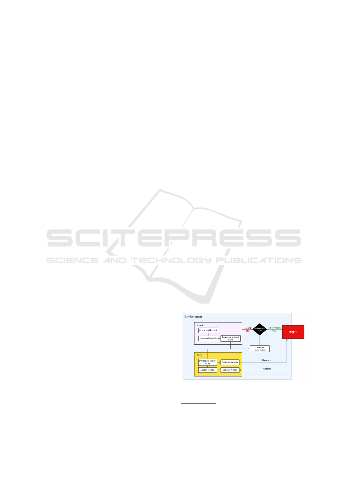
3.1.1 Episode Setup

The general idea of the setup is that the collision set-

ting is created ﬁrst. The position of the satellite is

created at a speciﬁc location, then the location of the

piece of debris is created in its vicinity, to ensure the

collision, and then their states are propagated back-

wards. These 3 processes are described below.

Satellite Orbit Creation

The orbit of the satellite is created by deﬁning the 6

Keplerian elements and the corresponding time epoch

that uniquely describes the position of the satellite in

time and space. The default values for the ﬁrst 5 Ke-

plerian elements (i.e. excluding the true anomaly υ)

are by default set to the values speciﬁed in the Ta-

ble 1. The true anomaly (υ) and the corresponding

time epoch are randomly generated so that the agent

can learn its task regardless of the collision position

or time.

Figure 1: Schematic interaction between the Agent and the

Environment.

https://gymnasium.farama.org/index.html

https://github.com/zampanteymedio/

gym-satellite-trajectory

ICAART 2025 - 17th International Conference on Agents and Artiﬁcial Intelligence

1010

Table 1: Environment Parameters.

Name Value Unit

Satellite

Parameters

SMA (a) 6795 [km]

e 0.18 -

i 21.64 [°deg]

ω 22.02 [°deg]

Ω 60.0 [°deg]

υ 0.0 [°deg]

Mass 100.0 [kg]

Surface area 1.0 [m

]

Reﬂection index 2.0 -

Thruster force 0.1 [mN]

Thruster I

4000.0 [s]

Debris

Parameters

Debris mass 10.0 [kg]

Debris surface area 1.0 [m

]

Debris reﬂection index 2.0 -

Propagation

Parameters

Method Dormand Prince

Integrator min step 1.0

Integrator max step 200.0

Error threshold 1.0 [m]

Perturbations Not Applied

Scenario

Parameters

Time of collision 2023/06/16 - 00:00:00.0 [UTC]

Time to avoid collision 4.0 [days]

Collision Min Distance 2000.0 [m]

Time to return to initial orbit 4.0 [days]

Time step size 600.0 [s]

Piece of Debris Orbit Creation

The position vector ⃗r

and the velocity vector ⃗v

the debris piece, components of the state vector, are

generated using the state vector of the target satellite

at the TCA:

⃗r

=⃗r

+ 10.0 ·⃗r

∆

; ⃗r

∆

∼ Uniform(0,1)

⃗v

= −⃗v

+ 10.0 ·⃗v

∆

; ⃗v

∆

∼ Uniform(0,1)

(1)

where⃗r

and ⃗v

are the position vector and the veloc-

ity vector of the target satellite at the TCA. The veloc-

ity of the debris is chosen to be opposite to the target

satellite to avoid a long encounter collision.

Propagation to the Initial State

A numerical propagator is created for each of the 2

space objects, the target satellite and the piece of de-

bris. The propagator is created using the parameters

in the Table 1.

The initial state of the target satellite is set to four

days before the TCA. Therefore, the propagator as-

sociated with the target satellite is used to propagate

the state at the TCA of the target satellite 4 days into

the past. This total duration is discretized in time by

using the time step size mentioned in the Table 1.

Similarly, the initial state of the piece of debris is

propagated backwards. The position of the piece of

debris is only relevant in the vicinity of the collision

state. Therefore, the state of the piece of debris is only

propagated 40 minutes into the past, using the same

time step size as in the case of the target satellite.

3.1.2 Observation Generation

The observation represents the information that the

agent receives from the environment based on the cur-

rent state. The observation is made up of four main

components:

• State of the target satellite object;

• State of the piece of debris;

• Time until collision;

• Amount of fuel consumed;

The encoding of the information related to these four

components is given to the agent using different ap-

proaches, with the differences between the two shown

in the Table 5.

Collision Avoidance and Return Manoeuvre Optimisation for Low-Thrust Satellites Using Reinforcement Learning

1011

3.1.3 Actions

In each step, the agent has the option of controlling

the thrusters of the target satellite, which are ﬁred for

the entire duration of the time step at the thrust level

selected by the agent. The thrust vector is projected

onto the three orthogonal axes that deﬁne the refer-

ence frame (either the GCRF or VNC, as given in the

Table 5).

3.1.4 Reward System

The reward system is one of the most important things

in a reinforcement learning setup, as it speciﬁes the

goal that the agent must achieve. The goals on which

the rewards are based are the following:

1. Collision Avoidance. The minimum distance be-

tween the target satellite and the debris must be

greater than a certain threshold value ∆r

2. Return to Original Orbit. The maximum dif-

ference between the ﬁnal Keplerian elements and

the initial elements must be smaller than a set of

thresholds (∆r

, ∆r

Ω

3. Fuel Consumption. The fuel consumed by the

satellite’s engines must be minimized.

4. Realism. For the duration of the event, the satel-

lite must follow orbits that are not too low (impact

on Earth) and not too high (leaving LEO).

During the development phase, the values of the

thresholds and the speciﬁc steps at which the rewards

are returned have changed. However, the function that

calculates the reward signal has the general form:

R = −(W

· r

+ R

ret

· r

+ R

bound

) (2)

The components of the reward signal are detailed be-

low:

• W

, r

: The weight and reward contribution corre-

sponding to (not) avoiding the collision:

= max(∆r

− min(∥⃗r

t,i

−⃗r

d,i

∥),0)

∆r

= 2000 [m]

(3)

where ”i” stands for all epochs in which the posi-

tion vector of the debris is known. W

varies de-

pending on the approach, speciﬁc values are given

in the Table 5.

• R

ret

: The return corresponding to the (non-)return

to the original orbit. 2 approaches have been de-

ﬁned:

Approach-1:

ret

(a,e,i,ω,Ω)

∑

0.2 ·C

(4)

(

0, if ∆

< ∆r

1, Otherwise

Approach-2:

ret

(a,e,i,ω,Ω)

∑

· max(∆

− ∆r

,0) (5)











0.002, k = a

0.01, k = e

0.01, k = i

0.1, k = ω

0.001, k = Ω

where ∆

is the absolute difference between the

current Keplerian element k and the original el-

ement. ∆r

is the corresponding threshold value

for the k element. Speciﬁc values for ∆r

can be

found in section 4, in the Table 5.

• W

, r

: The weight and premium contribution de-

pending on fuel consumption:

= (M

− M

)/M

= 10000

(6)

where M

and M

are the original and current mass

of the satellite.

• R

bound

: The return corresponding to leaving the

orbital boundaries:

bound

(

0 , if 6500 < ∥⃗r

target

∥ < 8000 [km]

10 , otherwise

(7)

3.2 Agent Implementation

The agent is an algorithm that is able to perform ac-

tions in certain states and improve the quality of these

actions based on the rewards received from the envi-

ronment. There are 3 algorithms that serve as agents

in the environment described in the previous section:

REINFORCE, DQN and PPO.

3.2.1 REINFORCE

REINFORCE is one of the simplest RL algorithms

that can be implemented. It is an on-policy algorithm,

i.e. the policy that is optimized is also the one used

to select actions in training. In this scenario, the al-

gorithm is used for the continuous action space, al-

though it could have been used for the discrete action

space.

The policy is a neural network which outputs the

mean (µ) and standard deviation (std) of the distribu-

tions from which the action components are selected.

ICAART 2025 - 17th International Conference on Agents and Artiﬁcial Intelligence

1012

The discount factor γ is a measure of how much rel-

evance current actions have for future rewards and

the number of training steps represents the number of

episodes used for training before an episode is used

purely for evaluation. The hyperparameters used for

the REINFORCE algorithm are speciﬁed in the Table

Table 2: Hyperparameters used in the REINFORCE algo-

rithm.

Hyperparameter Name Value

Discount factor γ 0.99

Number of training steps 5

Hidden Layer 1 size 128

Hidden Layer 2 size 64

Optimiser Adam

Learning rate 0.01

3.2.2 Deep Q-Network

The Deep Q-Network (DQN) algorithm is an off-

policy algorithm, in contrast to the previously pre-

sented one. DQN uses a ε greedy approach for select-

ing actions during training. It is also an algorithm that

can only be used in the context of discrete actions:

a = (a

), with a

∈ {−1,0,1}

(8)

In the DQN implementation, both the policy net-

work (Q-net) and the target network are neural net-

works with identical architectures but different pa-

rameters. They output the expected reward for each

action. A key feature in the current implementation

is the addition of a normalization layer. In Approach-

1, observations were normalized in the environment,

while in Approach-2, normalization was handled by a

normalisation layer added to the network.

The replay memory (R

) is used, which stores

experiences in a double-ended queue (”deque”) and

randomly selects them for model updates. To sta-

bilize training, the gradients of the Q-net parame-

ters are truncated to prevent excessive gradient norms.

The hyperparameters used in the implementation of

the DQN algorithm for the 2 different approaches are

listed in the Table 3.

3.2.3 Proximal Policy Optimization

The PPO algorithm uses a combination of a policy

gradient algorithm, called Actor, and a value-based

algorithm, called Critic. The PPO algorithm imple-

mented in this article is used in a continuous space

and follows the implementation developed in (Schul-

man et al., 2017). The reason for choosing PPO is its

stability in the training process, which results from the

Table 3: Hyperparameters used in the DQN algorithm.

Hyperparameter

Name

Value

Apr. 1

Value

Apr. 2

Action space [-1, 0, 1] [-1, 0, 1]

Batch size 128 128

Replay Memory size 10000 10000

Discount factor γ 0.99 0.99

start

0.9 0.9

end

0.05 0.05

decay

1000 100000

τ 0.005 0.005

Norm Layer No Yes

Hidden Layer 1 size 500 128

Hidden Layer 2 size 200 64

Optimiser Adam Adam

Learning rate 0.0001 0.0001

Clip Norm 5 5

update strategy used for the actor. The neural network

used to represent the actor (the policy) is designed us-

ing the hyperparameters given in the Table 4.

Table 4: Hyperparameters used in the PPO algorithm.

Hyperparameter Name Value

Steps per epoch 5 x 1151 (5 episodes)

Discount factor γ 0.99

GAE λ factor 0.97

Maximum KL 0.025

Maximum optimisation steps 80

Clip ratio ε 0.2

Learning rate actor 0.0003

Learning rate critic 0.001

Actor Hidden Layer 1 size 128

Actor Hidden Layer 2 size 64

Critic Hidden Layer 1 size 64

Optimiser Adam

4 EVALUATION

This section presents the results obtained by train-

ing the three RL algorithms presented in the previ-

ous section with the two main approaches developed.

Approach-1 represents the ﬁrst set of parameters that

showed relevant results, while Approach-2 represents

the ﬁnal set of parameters that showed the best re-

sults in the more restrictive setting. Approach-2 is an

improvement over Approach-1. The main differences

between the two approaches are described in the Ta-

ble 5.

The models are compared both quantitatively and

qualitatively. The evaluation of an agent includes:

• Raw Reward Sum: The sum of the rewards re-

ceived for the duration of an episode. This value

is averaged over 30 independent runs.

Collision Avoidance and Return Manoeuvre Optimisation for Low-Thrust Satellites Using Reinforcement Learning

1013

• Collision Avoidance Status: The collision must

be avoided under all circumstances.

• Return to Original Orbit: The evolution of the

ﬁrst 5 Keplerian elements is analyzed quantita-

tively and qualitatively. The agent returns to the

original orbit if all elements in the ﬁnal state are

within the speciﬁed threshold values.

• Fuel Consumption: If all previous conditions are

met, a model with lower fuel consumption is pre-

ferred.

• Action Choices: The agent that performs the

fewest actions and has a smoother action change

is preferred.

4.1 Approach-1 Results

The algorithms REINFORCE, DQN and PPO have

been trained and the test results are available in the Ta-

ble 6. The columns ”Collision Avoided” and ”Returns

to Orbit” show the percentage of episodes in which

the agent reached the corresponding target, while the

column ”Fuel Used” shows the percentage of fuel

used out of the total amount that could potentially

have been used.

The table shows that the DQN algorithm per-

formed best of the three algorithms. However, the

goals that had to be achieved were not very restrictive

for Approach-1 - see Table 5. The thresholds deﬁning

the initial orbit are rather loose, which is one of the

reasons why the model seemed to perform so well.

In fact, not all episodes return to the initial orbital el-

ements - in some cases the elements deviate further

from the initial elements. However, since the thresh-

olds are not very restrictive, the ﬁnal orbit was still

within the appropriate range to be called equivalent

to the initial orbit. Approach-2 addresses some of the

issues observed with this ﬁrst approach.

4.2 Approach-2 Results

In Approach-2, emphasis was placed on the task of

returning to the initial orbit. The steps at which the re-

turn was rewarded (or penalized) were increased and

the thresholds were signiﬁcantly lowered (see Table

5) to penalize excessive deviations. In addition, the

reward contribution of the return to the initial orbit

component has been changed to be optimizable in-

stead of a step function (Equation 5). This is all done

to incentivize the agent to return to the initial orbit.

The observation structure was changed, as was

the reference frame of the manoeuvre presentation,

as described in the Table 5. The test results ob-

tained with Approach-2 are shown in the Table 7.

The results are not directly comparable with those of

Table 5: Implementation differences between approaches.

Element Approach-1 Approach-2

Satellite state representation Cartesian Coordinates - GCRF Keplerian Elements

Piece of debris representation Sequence of State-Vectors Estimated min. distance (between

satellite and debris)

Manouevre Thrust Components GCRF ref. frame VNC ref. frame

Coll. Avoid. reward weight (W

) 0.01 0.0005

Return to Orbit Thresholds

Semi-major axis (∆r

) 500.0 [m] 10.0 [m]

Eccentricity (∆r

) 0.001 1e-8

Inclination (∆r

) 1.0 [rad] 1e-8 [rad]

Argument of Perigee (∆r

) 10.0 [rad] 10.0 [rad]

RAAN (∆r

Ω

) 1.0 [rad] 1e-8 [rad]

Table 6: Agents comparison averaged over 30 episodes - Approach-1.

Rewards Sum Rewards Std Coll. Avoided [%] Orbit Return [%] Fuel Used [%]

REINF. -3.28 0.10 100 70 84.18

DQN -0.68 0.19 100 100 16.6

PPO -2.34 0.74 100 3 22.62

Table 7: Agents comparison averaged over 30 episodes - Approach-2.

Rewards Sum Rewards Std Coll. Avoided [%] Orbit Return [%] Fuel Used [%]

REINF. -1301.48 67.22 100 0 78.29

DQN -258.51 74.44 100 0 52.83

PPO -175.23 11.59 100 0 38.49

ICAART 2025 - 17th International Conference on Agents and Artiﬁcial Intelligence

1014

Approach-1, as the reward system and the observa-

tion structure differ signiﬁcantly. The task of return-

ing to the original orbit was also not fulﬁlled by all

models in all episodes performed, which is expected

given the extremely strict thresholds. Qualitatively,

all agents trained according to Approach-2 performed

better than the agents trained according to Approach-

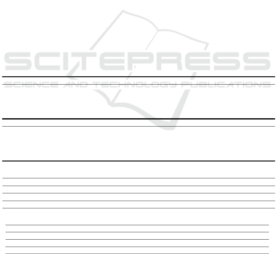
Just looking at the numbers, it looks like the

PPO model achieves the best overall results with

Approach-2. It has the highest reward sum over the

evaluation episodes, the smallest standard deviation

and the lowest fuel consumption. However, when

looking at the evolution of the Keplerian elements and

the action proﬁles (Figures 2 - 5), the DQN model

is the clear favorite. The development of the Kep-

lerian elements follows the same pattern in almost

all episodes as in Figure 2 for the DQN model: a

clear, steady increase in the absolute magnitudes of

the differences to the initial elements, followed by

a steady decline, almost to the same starting point.

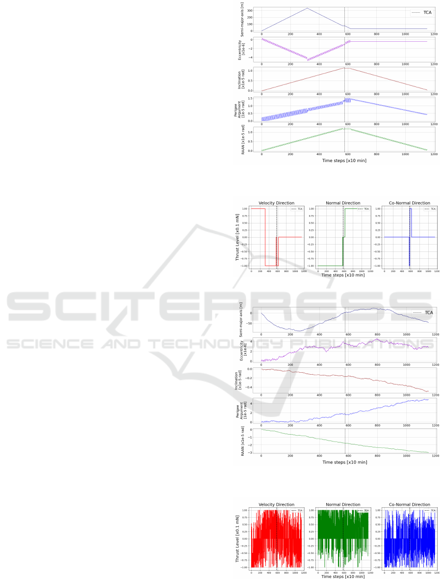
Looking at the action proﬁles in Figure 3, there are

also no rapid ﬂuctuations or long periods of ﬂuctua-

tion. These rapid ﬂuctuations are however present in

the manoeuvres computed by the PPO model. This

is expected, given the model operates in the continu-

ous action space setting. Even though the PPO model

obtains the best results quantitatively, the sequence of

manoeuvres given by the model are unpractical.

5 CONCLUSIONS

This paper presents an algorithm for collision avoid-

ance and return manoeuvres for a low-thrust satel-

lite in Low-Earth orbit, using reinforcement learning

(RL). A simulated environment allowed the agents to

learn from different states and optimize thruster con-

trol to avoid collisions, return to the original orbit, and

minimize fuel consumption.

Three algorithms were tested: REINFORCE, PPO

(for the continuous action space), and DQN (for the

discrete action space). Two approaches were ex-

plored. In Approach-1, satellite states and actions

were given in the GCRF reference frame, and the

agent received sparse rewards. Approach-2 used Ke-

plerian elements, frequent rewards, and stricter goals.

All algorithms avoided collisions, but returning to the

initial orbit was challenging, especially in the con-

tinuous action space. The PPO algorithm favored

fuel efﬁciency, while DQN succeeded in both tasks,

though often at a higher fuel cost. The discrete ac-

tion space formulation proved easier to implement

and more effective for the task.

Figure 2: Keplerian Elements Variation - DQN Approach-2

(Best Model Qualitatively).

Figure 3: Agent Actions - DQN Approach-2.

Figure 4: Keplerian Elements Variation - PPO Approach-2

(Best Model Quantitatively).

Figure 5: Agent Actions - PPO Approach-2.

Collision Avoidance and Return Manoeuvre Optimisation for Low-Thrust Satellites Using Reinforcement Learning

1015

Ultimately, the DQN algorithm in Approach-2

provided the best results, showing that RL can ef-

fectively optimize collision avoidance and return ma-

noeuvres for low-thrust satellites.

ACKNOWLEDGMENT

We thank the International Astronautical Congress,

IAC 2024, Milan, Italy, October 14-18, 2024, for

feedback offered on a preliminary form of this work.

This research is partially supported by the project

“Romanian Hub for Artiﬁcial Intelligence - HRIA”,

Smart Growth, Digitization and Financial Instru-

ments Program, 2021-2027, MySMIS no. 334906

and a grant of the Ministry of Research, Innovation

and Digitization, CNCS/CCCDI-UEFISCDI, project

no. PN-IV-P8-8.1-PRE-HE-ORG-2023-0081, within

PNCDI IV.

REFERENCES

B. Gaudet, R. Linares, R. F. (2020). Six degree-of-freedom

body-ﬁxed hovering over unmapped asteroids via li-

dar altimetry and reinforcement meta-learning. Acta

Astronautica, 172:90–99.

Boscolo Fiore, N. (2021). Machine Learning based Satellite

Collision Avoidance strategy. PhD thesis, Politecnico

Milano.

Casas, C. M., Carro, B., and Sanchez-Esguevillas, A.

(2022). Low-thrust orbital transfer using dynamics-

agnostic reinforcement learning.

D. M. Novak, M. V. (2011). Improved shaping approach to

the preliminary design of low-thrust trajectories. Jour-

nal of Guidance, Control, and Dynamics.

Gaudet, B., Linares, R., and Furfaro, R. (2020). Adaptive

guidance and integrated navigation with reinforce-

ment meta-learning. Acta Astronautica, 169:180–190.

Holt, H., Armellin, R., Baresi, N., Hashida, Y., Turconi, A.,

Scorsoglio, A., and Furfaro, R. (2021). Optimal q-

laws via reinforcement learning with guaranteed sta-

bility. Acta Astronautica, 187:511–528.

Kolosa, D. S. (2019). A Reinforcement Learning Approach

to Spacecraft Trajectory Optimization. PhD thesis,

Western Michigan University.

LaFarge, N. B., Miller, D., Howell, K. C., and Linares, R.

(2021). Autonomous closed-loop guidance using re-

inforcement learning in a low-thrust, multi-body dy-

namical environment. Acta Astronautica, 186:1–23.

Mnih, V. et al. (2013). Playing atari with deep reinforce-

ment learning. https://arxiv.org/abs/1312.5602.

N. Bourriez, A. Loizeau, A. F. A. (2023). Spacecraft au-

tonomous decision-planning for collision avoidance :

a reinforcement learning approach. 74th INTERNA-

TIONAL ASTRONAUTICAL CONGRESS (IAC).

Pinto, F. et al. (2020). Towards automated satellite con-

junction management with bayesian deep learning.

Proceedings of NeurIPS 2020, AI for Earth Sciences

Workshop.

Schulman, J., Wolski, F., Dhariwal, P., Radford, A., and

Klimov, O. (2017). Proximal policy optimization al-

gorithms. Arxiv.org/abs/1707.06347.

Sutton, R. S. and Barto, A. G. (2018). Reinforcement Learn-

ing: An Introduction. MIT Press, Cambridge, MA,

2nd edition.

Tipaldi, M., Iervolino, R., and Massenio, P. R. (2022). Rein-

forcement learning in spacecraft control applications:

Advances, prospects, and challenges. Annual Reviews

in Control, 54:1–23.

Whiffen, G. (2006). Mystic: Implementation of the

static dynamic optimal control algorithm for high-

ﬁdelity, low-thrust trajectory design. Proceedings of

AIAA/AAS Astrodynamics Specialist Conference and

Exhibit.

Yang, C., Zhang, H., and Gao, Y. (2021). Analysis of

a neural-network-based adaptive controller for deep-

space formation ﬂying. Advances in Space Research,

68(1):54–70.

Zavoli, A. and Federici, L. (2021). Reinforcement learn-

ing for robust trajectory design of interplanetary mis-

sions. Journal of Guidance, Control, and Dynamics,

44(8):1440–1453.

ICAART 2025 - 17th International Conference on Agents and Artiﬁcial Intelligence

1016