Principal Direction 2-Gaussian Fit
Nicola Greggio and Alexandre Bernardino
Instituto de Sistemas e Rob
´
otica, Instituto Superior T
´
ecnico, 1049-001 Lisbon, Portugal
Keywords:
Unsupervised Clustering, Gaussian Mixture Models, Greedy Methods, Ill-Posed Problem, Splitting
Components.
Abstract:
In this work we address the problem of Gaussian Mixture Model estimation with model selection through
coarse-to-fine component splitting. We describe a split rule, denoted Principal Direction 2-Gaussian Fit, that
projects mixture components onto 1D subspaces and fits a two-component model to the projected data. Good
split rules are important for coarse-to-fine Gaussian Mixture Estimation algorithms, that start from a single
component covering the whole data and proceed with successive phases of component splitting followed by
EM steps until a model selection criteria is optimized. These algorithms are typically faster than alternatives
but depend critically in the component splitting method. The advantage of our approach with respect to other
split rules is twofold: (1) it has a smaller number of parameters and (2) it is optimal in 1D projections of the
data. Because our split rule provides a good initialization for the EM steps, it promotes faster convergence
to a solution. We illustrate the validity of this algorithm through a series of experiments, showing a better
robustness to the choice of parameters this approach to be faster that state-of-the-art alternatives, while being
competitive in terms of data fit metrics and processing time.
1 INTRODUCTION
Unsupervised clustering classifies different data into
classes based on redundancies contained within the
data sample. The classes, also called clusters, are de-
tected automatically, but often the number of compo-
nents must be specified a priori. Many approaches
exist: Kohonen maps Kohonen (1982a) Kohonen
(1982b), Growing Neural gas Fritzke (1995), Holm-
str
¨
om (2002), K-means MacQueen (1967), Indepen-
dent component analysis Comon (1994), Hyv
¨
arinen
et al. (2001), etc. One of the most prominent ap-
proaches consists fitting to the data a mixture of statis-
tical distributions of some kind (e.g. Gaussians). Fit-
ting a mixture model to the distribution of the data is
equivalent, in some applications, to the identification
of the clusters with the mixture components McLach-
lan and Peel (2000). Learning the mixture distribution
means estimating the parameters of each of its com-
ponents (e.g. prior probability, mean and covariance
matrix in case of a Gaussian component).
To learn a mixture model, a particularly successful
approach is the Expectation Maximization (EM) al-
gorithm McLachlan and Peel (2000), Hartley (1958),
McLachlan and Bashford (1988), McLachlan and T.
(1997). Its key property is its assured convergence
to a local optimum Dempster et al. (1977), especially
for the case of Normal mixtures McLachlan and Peel
(2000), Xu and M. (1996). However, it also presents
some drawbacks. For instance, if requires the a-priori
specification of the model order, (the number of com-
ponents), and its results are sensitive to initialization.
Determining the mixture complexity, i.e. the se-
lection of the right number of components, is not triv-
ial. The more components there are within the mix-
ture, the better the data fit will be. However, a higher
number of components will lead to data overfitting
and a waste of computation. Hence, the best com-
promise between precision, generalization and speed
is difficult to achieve. A common approach is to es-
timate several mixtures, all with different number of
components, and then select the best model according
to some appropriate criteria. However, this strategy
is quite computationally intensive and a few methods
have been proposed to integrate the model selection
criteria in the mixture estimation process. Some of
the most efficient methods adopt the paradigm of in-
cremental split methods Greggio et al. (2010) Greggio
et al. (2014), that start with a single component and
progressively adapts the mixture by adding new el-
ements based on individual component splitting fol-
lowed by EM steps to converge to a local optimum.
Greggio, N. and Bernardino, A.
Principal Direction 2-Gaussian Fit.
DOI: 10.5220/0013250400003905
Paper published under CC license (CC BY-NC-ND 4.0)
In Proceedings of the 14th International Conference on Pattern Recognition Applications and Methods (ICPRAM 2025), pages 309-317
ISBN: 978-989-758-730-6; ISSN: 2184-4313
Proceedings Copyright © 2025 by SCITEPRESS – Science and Technology Publications, Lda.
309

The process stops when an appropriate model selec-
tion criteria is optimized.
1.1 Related Work
The selection of the mixture complexity is essential in
order to prevent overfit, finding the best compromise
between the accuracy of the data description and the
computational burden. There are different strategies
for determining the number of components in a mix-
ture. Split-based algorithms usually start with a sin-
gle component, and then increase their number during
the computation, by splitting existing components in
two new components at each stage. Since splitting a
component is an ill-posed problem, several methods
have been proposed in the literature. It has not yet
been found a theoretical way to assess the quality of a
particular algorithm so most works to assess it empir-
ically, using numerical simulations to measure preci-
sion and computational efficiency. Greedy strategies
have been proved mathematically to be effective in
learning a mixture density by maximum likelihood,
i.e. by incrementally adding components to the mix-
ture up to a certain number of components k.
In 2000, Li and Barron demonstrated that, in
case of mixture density estimation, a k-component
mixture learnt via maximum likelihood estimation
- or by an iterative likelihood algorithm - achieves
log-likelihood within order 1/k of the log-likelihood
achievable by any convex combination Li and Barron
(2000). However, the big drawback in these kind of
algorithms is the imprecision of the split criterion.
In 1999, Vlassis and Likas proposed an algo-
rithm that employs splitting operations for mono-
dimensional Gaussian mixtures, based on the evalu-
ation of the fourth order moment (Kurtosis) Vlassis
and Likas (1999). They assumed that if a component
has a Kurtosis different to that of a regular Gaussian,
then this subset of points may be better described by
more than a single component. Their splitting rule as-
signs half of the old component’s prior to the two new
one, and the same variance as the old one, while dis-
tancing the two means by one standard deviation with
respect to the old mean.
In 2002 Vlassis and Likas introduced a greedy al-
gorithm for learning Gaussian mixtures Vlassis and
Likas (2002). It starts with a single component cover-
ing all the data. However, their approach suffers from
being sensitive to a few parameters that have to be
fine-tuned. The authors propose a technique for opti-
mizing them. Nevertheless, the latter brings the total
complexity for the global search of the element to be
split O(n
2
), being n the number of input data points.
Subsequently, following this approach, Verbeek et
al. developed a greedy method to learn the mixture
model Verbeek et al. (2003) where new components
are added iteratively, and the EM is applied until it
reaches the convergence. The global search for the
optimal new component is achieved by starting ’par-
tial’ EM searches, each of them with different initial-
izations. Their approach is based on describing the
mixture by means of a parametrized equation, whose
parameters are locally optimized (rather than globally,
for saving computation resources. The real advantage
with respect to the work in Vlassis and Likas (2002)
is that the computational burden is reduced.
Considering the techniques that both increase and
reduce the mixture complexity, there are different
approaches in literature. In particular, Richardson
and Green used split-and-merge operations together
with birth and death operations to develop a re-
versible jump method and constructed a reversible
jump Markov chain Monte Carlo (RJMCMC) algo-
rithm for fully Bayesian analysis of univariate gaus-
sians mixtures Richardson and Green (1997). The
novel RJMCMC methodology elaborated by Green is
attractive because it can preferably deal with param-
eter estimation and model selection jointly in a sin-
gle paradigm. However, the experimental results re-
ported in Richardson and Green (1997) indicate that
such sampling methods are rather slow as compared
to maximum likelihood algorithms.
Ueda et al. proposed a split-and-merge EM al-
gorithm (SMEM) to alleviate the fact that EM con-
vergence is local and not global Ueda et al. (2000).
They defined the merge of two components as a lin-
ear combination of them, in terms of their parameters
(priors, means and covariance matrices), with the pri-
ors as weights. Therefore, the splitting operation is
the inverse, where there is the need for finding the op-
timal weights. Their splitting operations are based on
the component-to-split’s covariance matrix decompo-
sition (they proposed both a method based on the
SVD and the other on the Cholesky decomposition).
Zhang et al. introduced another split-and-merge
technique, based on that of Ueda et al. Zhang et al.
(2003). As a split criterion they define a local Kull-
back divergence as the distance between two distribu-
tions: the local data density around the model with
k components (k
th
model) and the density of the k
th
model specified by the current parameter estimate.
The local data density is defined as a modified em-
pirical distribution weighted by the posterior proba-
bility so that the data around the k
th
model is focused
on. They employ the technique of the Ueda’s SMEM
algorithm Ueda et al. (2000), modifying the part that
performs the partial EM step to reestimate the param-
eters of components after the split and merge opera-
ICPRAM 2025 - 14th International Conference on Pattern Recognition Applications and Methods
310

tions. These components are re-estimated without af-
fecting the other components that do not participate in
the split and merge procedure. The authors claim this
helps to reduce the effects the linear heuristic split-
and-merge methods result in. However, both methods
results in some equations that depend, for each split,
on three empirical values.
An interesting approach is that of Constantinopou-
los and Likas Constantinopoulos and Likas (2007).
They first apply a variational model until conver-
gence, removing those components that do not con-
tribute to the data description. Then, after conver-
gence, they, for each remaining component - if there is
more than one component left - split each single com-
ponent into two new ones, and then optimize this 2-
component mixture locally with the variational algo-
rithm. Regarding the splitting procedure, they place
the centers of the two components along the dimen-
sion of the principal axis of the old component’s co-
variance and at opposite directions with respect to the
mean of the old component, while the priors are both
half of the old one.
In 2011, Greggio et al. Greggio et al. (2011)
proposed the FASTGMM method, a fast split-only
method for GMM estimation with model selection.
The key idea is to speed up split-based methods by
realizing that split moves can be made without wait-
ing for complete adaptation of the mixture (conver-
gence of the EM steps) at each model complexity.
This method showed good results in image segmenta-
tion problems, where computational efficiency issues
should be taken into consideration, but it yields a sig-
nificant number of parameters to tune.
In Greggio et al. (2010) and Greggio et al. (2014),
we have introduced the FSAEM algorithm, which
performs sequential splits along the directions of the
component’s eigenvectors in descending order of the
eigenvalues magnitudes. However, the split rule ini-
tializes the two new components using a fixed rule
based on the parameters of the original component.
The use of fixed split rules is common in other meth-
ods such as Zhang et al. (2003), Huber (2011), and
Zhao et al. (2012), but, depending on the characteris-
tics of the data, the subsequent EM steps may take a
long time to converge. More recently, in Greggio and
Bernardino (2024), we have proposed the FSAEM-
EM algorithm, which splits a component based on an
optimal two-Gaussian fit to the projection of the com-
ponents points into a 1D subspace. This rule, despite
being only optimal for the 1D case, was shown to
significantly reduce the number of computations for
similar precision levels even in the multidimensional
case.
1.2 Our Contribution
In this paper we follow upon our previous work Greg-
gio and Bernardino (2024) and present several op-
timizations leading to improved computational effi-
ciency. A sequence of Gaussianity tests (e.g. Lil-
liefors Lilliefors (1967)) are applied to the compo-
nents prior to splitting to avoid unnecessary compu-
tations. The tests are optimized both for the initial
multidimensional component as well as for the 1D
components resulting from the projections along the
eigenvectors’ directions. On the one hand, we can ex-
clude from splitting those components that are already
Gaussian and splitting will not improve the descrip-
tion of the data. On the other hand, the Lilliefors tests
on the 1D projections are sorted and used to priori-
tize the directions of split. Thus, the first directions
to split will be the ones that most contribute to the
non-normality of the selected data. These contribu-
tions lead to a faster algorithm, called it FSAEM-EM-
L, which has a comparable accuracy to FSAEM-EM.
New tests illustrate the effectiveness of our proposal.
1.3 Outline
In section 1.1 we analyze the state of the art of un-
supervised learning of mixture models. In section 2
we introduce the new proposed algorithm, while in
sec. 2.2 we specifically address our splitting proce-
dure. Then, in section 3 we describe our experimental
set-up for testing the validity of our new technique,
and we compare our results against our previous al-
gorithm FSAEM. Finally, in section 4 we conclude
and propose directions for future work.
2 MIXTURE LEARNING
ALGORITHM: PRINCIPAL
DIRECTION 2-GAUSSIAN FIT
In this section we describe the proposed algorithm. It
is based on our previous work FSAEM-EM Greggio
and Bernardino (2024), with additional computational
improvements. We call it Principal Direction 2 Gaus-
sian Fit, or, schematically, FSAEM-EM-L, in order
to enhance the analogy with the previous algorithm,
FSAEM-EM, while being able to distinguish this new
formulation from the latter.
2.1 Algorithm Outline
This algorithm starts with a single component, hav-
ing the mean and covariance matrix of the whole in-
Principal Direction 2-Gaussian Fit
311

put data set. Then, a sequence of recursive compo-
nent splits is performed until a cost function based on
the MML criterion is optimized. Each split operation
initializes two new components based on the original
(which is removed from the mixture). The EM is then
applied to the whole mixture until convergence. If
the cost function has not improved in this process, the
mixture is reverted to the previous stage, and a differ-
ent split operation is tried. The process stops if splits
have been tried on all components, along all eigenvec-
tors’ directions, without improving the cost function.
The main contribution of the current implemen-
tation is the use of Lilliefors tests prior to the deci-
sion of the component to split and to the split direc-
tions, to improve the computational efficiency of the
method. For each component the Lilliefors test is per-
formed along all the input dimensions. Then, we sort
these dimensions in descending order, based on the
results of the Lilliefors test, from that being the most
far from normality. Consequently, we start splitting
the component along that direction first, and then, in
case there is no improvement, along the other remain-
ing ordered directions.
2.2 The Splitting Procedure
The Principal Direction 2-Gaussian Fit algorithm
considers a split operation that projects the points of
the component to split in a single direction and fits
a 2-Component Gaussian on those points via EM.
Two main problems have to be dealt with: (i) deter-
mine which points belong to each component, and (ii)
choose a direction in which to project those points.
Regarding the first problems, ideally only the points
belonging to a particular component should be in-
volved in the EM steps. However, it is not possible
a priori to know which points belong to a component.
Our solution determines which component c each in-
put point x belongs to by evaluating each component’s
distribution at that point p
c
(x) weighted for each prior
w
c
, and then taking the highest value. Formally, this
is expressed by:
c
MAX
= arg max
c

w
c
p
c
(x)
p(x)

= arg max
c
(w
c
p
c
(x)), c = 1,2,... k
(1)
In this case, the global distribution p(x) can be omit-
ted, since it is constant across components at each
point and so, does not affect the final result. We con-
sider the point ¯x belonging to the component c
max
if
p
c
max
(x) < p
c
(x) with c ̸= i
max
, c = 1,2,. .. k.
Regarding the selection of the dimension to op-
erate along, we choose sequentially from the com-
ponents principal directions (the eigenvectors of its
covariance matris) sorted by decreasing value of the
Liliefors test statistic applied to the projected points.
Higher values indicate directions in which the com-
ponent deviated more from Gaussianity.
The problem is finding a 1D mixture with two
Gaussian components fitting points projected in the
principal directions. The advantage of our method is
obtaining this two-component-mixture efficiently by
taking advantage of one-dimensional data. This can
be done with the classical EM algorithm or variants.
In our experiments, we use the EM algorithm initial-
ized by the K-means algorithm, with 2 clusters as in-
put parameter. The K-means initial centroids are set
to the means of the subsets of points to the left and to
the right of the mean of the 1D projections.
Once the EM 1D has learned the parameters of
the two components, (w
1
,µ
1
,σ
1
) and (w
2
,µ
2
,σ
2
), we
bring them back to their original multidimensional
space. This is achieved by multiplying the origi-
nal component by the computed mixture of two 1-
dimensional Gaussians along the direction in which
the points were projected.
The classical representation of the multivariate
Gaussian distribution is:
p(x|µ,Σ) =
1
(2π)
d/2
|Σ|
1/2
exp
−
1
2
(x−µ)
T
Σ
−1
(x−µ)
(2)
where d is the dimension of the space. However, for
our purposes the canonical parameterization will be
more useful:
p(x|η,Λ) = exp
ξ+η
T
x−
1
2
x
T
Λx
(3)
where Λ = Σ
−1
, η = Σ
−1
µ and ξ =
−
1
2

d log2π −log|Λ| +η
T
Λ
−1
η

. The multi-
plication of two Gaussian distributions in the
canonical form is:
p
3
(x|η
3
,Λ
3
) = exp
ξ
3
+η
T
3
x−
1
2
x
T
Λ
−1
3
x
(4)
where η
3
= η
1
+ η
2
, Λ
3
= Λ
1
+ Λ
2
and ξ
3
=
−
1
2

d log2π −log|Λ
3
| + η
T
3
Λ
−1
3
η
3

. A and B are the
two multidimensional Gaussian components that sub-
stitute the old one, and 1 and 2 their corresponding
1D projections. In our case we have:
η
1
= Λ
1
µ
1
; η
2
= Λ
2
µ
2
; η = Λµ = Σ
−1
µ;
η
A
= η
1
+ η = σ
−1
1
+ Σ
−1
; η
B
= σ
−1
1
+ Σ
−1
Λ
A
= Λ
1
+ Λ = σ
−1
2
+ Σ
−1
; Λ
B
= σ
−1
2
+ Σ
−1
⇒ µ
A
= Λ
A
/η
A
; Σ
A
= Λ
−1
A
; w
A
= w · w
1
µ
B
= Λ
B
/η
B
; Σ
B
= Λ
−1
B
; w
B
= w · w
2
(5)
If the new mixture configuration is rejected after the
next MML evaluation, all the other dimensions will
be tried in order of decreasing Liliefors test statistic,
ICPRAM 2025 - 14th International Conference on Pattern Recognition Applications and Methods
312

until no further direction is left, then discarding the
current component.
The full splitting procedure pseudocode is shown
in Algorithm 1.
1: Input: input data, selected mixture component
2: Output: two-component local description mixture
3: Compute the principal directions of the selected com-
ponent – eigenvectors of the covariance matrix
4: Identify points corresponding to the selected mixture
component
5: project the selected points into the principal directions
6: Compute Liliefors test statistic for all principal direc-
tions
7: Sort the principal directions in decreasing order of the
test statistic
8: Test sequentially each sorted principal directions
9: cluster projected points with K-means, whose cen-
troids are the means of the first and second half subsets
10: run 1D-EM initialized by the K-means results
11: re-project the 1D two-components to the original mul-
tidimensional space
12: if data likelihood improves, move to another compo-
nent, otherwise try another principal direction.
Algorithm 1: Principal Direction 2-Gaussian Fit splitting
procedure.
2.3 Reaching a EM Local Optimum
In the practical application of the EM algorithm, iter-
ations are stopped when the total log-likelihood of the
data stabilizes (difference on consecutive iterations
are below some small threshold). However, the to-
tal log-likelihood of the input data does not provide a
complete view of the algorith convergence. In fact, it
may happen that while a component is evolving such
as to increase the data likelihood, other may be de-
creasing it. The net effect may be of stabilization
of the total log-likelihood, that would stop the pro-
cess prematurely, while the mixture is still evolving
towards a better representation. It is demonstrated
that the EM algorithm does not decrease the total
log-likelihood at consecutive iterations, but it is un-
clear what happens locally at each component of the
mixture. Therefore, it is important to consider the
log-likelihood evolution for each component, rather
than the whole mixture behavior in order to prevent
early stopping. Besides, this log-likelihood increment
should be considered in percentage, not only an ab-
solute value, because it is highly dependent on the
data distribution. This ensures that, before stopping
the EM optimization, no component is being updated,
therefore a local optimum is reached.
In our approach, at each new mixture configura-
tion (addition of new components by the splitting op-
eration) the EM algorithms is performed in order to
converge to a local optimum of that distribution con-
figuration. Once the mixture parameters
¯
ϑ are com-
puted, our algorithm evaluates the current likelihood
of each component c as:
Λ
curr
(c)
(ϑ) =
n
∑
i=1
ln(w
c
p
c
( ¯x
i
))
(6)
During each iteration, the algorithm keeps mem-
ory of the previous likelihood of each mixture com-
ponent Λ
last
(c)
(ϑ).
Then, we define our stopping criterion for the EM
algorithm when all components have stabilized, i.e.:
Λ
incr
(c)
(ϑ) =




Λ
curr
(c)
(ϑ) − Λ
last
(c)
(ϑ)
Λ
curr
(c)
(ϑ)




100
c
∑
i=1


Λ
incr
(i)
(ϑ)


⩽ δ
(7)
where here Λ
incr
(c)
(ϑ) denotes the percentage incre-
ment in log-likelihood of the component c, | · | is the
module, or absolute value of (·), and δ is the value
of the minimum percentage increment. We choose
δ = 0.001, which implies δ
%
= 0.1%. Analogously,
we set the minimum percentage increment of the 1D
EM as δ
1D
= 1/δ = 0.0001.
3 EXPERIMENTAL VALIDATION
AND DISCUSSION
We will compare our Principal Direction 2 Gaus-
sian Fit, herein called FSAEM-EM-L, to our previous
work FSAEM-EM, in order to validate the effect the
application of the Lilliefors test has on the computa-
tional complexity of the whole algorithm. We are in-
terested in evaluating how this new approach can im-
prove, in terms of precision of data description, and
computational time.
3.1 Quantitative Ground Truth
Comparison Evaluation
A deterministic approach for comparing the differ-
ence between the original mixture and the estimated
one is to adopt a unique distance measure between
probability density functions. Jensen et al. (2007) ex-
posed three different strategies for computing such
distance: The Kullback-Leibler divergence, the Earth
Mover’s distance, and the Normalized L2 distance.
The first one is not symmetric, even though a sym-
metrized version is usually adopted Jensen et al.
(2007). However, this measure can be evaluated in a
closed form only with mono-dimensional gaussians.
The second one also suffers analog problems. The
Principal Direction 2-Gaussian Fit
313

2D data
3-components 5-components
FSAEM-EM FSAEM-EM-L FSAEM-EM FSAEM-EM-L
Lilliefors: NO Lilliefors: YES Lilliefors: NO Lilliefors: YES
-4 -2 0 2 4
-6
-4
-2
0
2
4
6
-4 -2 0 2 4
-6
-4
-2
0
2
4
6
-4 -2 0 2 4
-4
-2
0
2
4
-4 -2 0 2 4
-4
-2
0
2
4
6-components 10-components
FSAEM-EM FSAEM-EM-L FSAEM-EM FSAEM-EM-L
Lilliefors: NO Lilliefors: YES Lilliefors: NO Lilliefors: YES
-6 -4 -2 0 2 4 6
-4
-2
0
2
4
6
-6 -4 -2 0 2 4 6
-4
-2
0
2
4
6
-4 -2 0 2 4
-4
-2
0
2
4
-4 -2 0 2 4
-4
-2
0
2
4
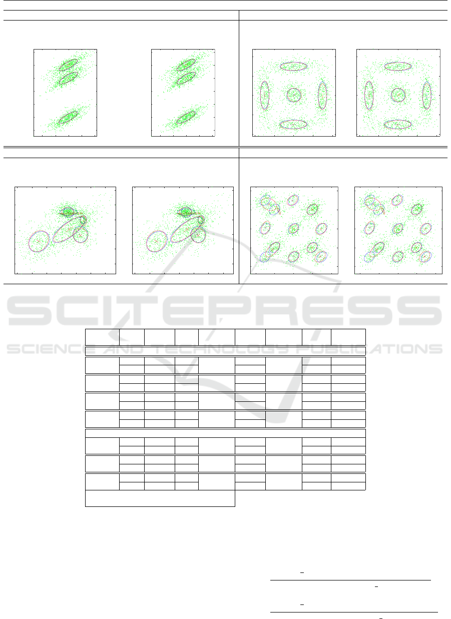
Figure 1: 2D synthetic data - For each plot set: generation mixture (blue) and the evaluated one (red) on the same input sets.
Table 1: Best values for experimental results on synthetic data.
Input L-test
# detect
# iter
perc. diff.
time [s]
perc. diff.
log-lik
Norm L2
comps. iter. [%] time [%] Distance
2D Synthetic data
3-comp
No 4 1318
92.41
12.82
74.34
-7237 0.0054
Yes 3 100 3.29 -7248 0.0032
5-comp
No 5 5037
67.54
33.10
69.85
-7237 0.0094
Yes 5 1635 1.446 -7659 0.0094
6-comp
No 6 3178
0.0
34.43
31.27
-7788 0.0305
Yes 6 3178 23.63 -7788 0.0305
12-comp
No 11 2785
26.89
25.48
24.18
-7582 0.0436
Yes 11 2036 19.32 -7592 0.0418
3D Synthetic data
3-comp
No 3 6000
98.73
38.97
92.12
-11220 0.0035
Yes 3 76 3.07 -11220 0.0035
5-comp
No 5 979
71.30
11.28
55.59
-12555 0.0056
Yes 5 281 5.01 -12555 0.0056
11-comp
No 12 5069
69.03
64.39
66.67
-15983 0.0296
Yes 10 1570 21.46 -16118 0.0777
mean iterations = 60.84 [iter] ± std = 38.55 [iter.]
mean time = 59.16 [s] ± std = 26.19 [s]
third choice, finally is symmetric, obeys to the trian-
gle inequality and it is easy to compute, with a pre-
cision comparable to the other two. Its expression is
given by Ahrendt (2005):
z
c
N
x
(¯µ
c
,
¯
Σ
c
) = N
x
(¯µ
a
,
¯
Σ
a
)N
x
(¯µ
b
,
¯
Σ
b
) (8)
where
¯
Σ
c
= (
¯
Σ
−1
a
+
¯
Σ
−1
b
)
−1
¯µ
c
=
¯
Σ
c
(
¯
Σ
−1
a
¯µ
a
+
¯
Σ
−1
b
¯µ
b
)
z
c
=
exp

−
1
2
(¯µ
a
− ¯µ
b
)
T
¯
Σ
−1
a
¯
Σ
c
¯
Σ
−1
b
(¯µ
a
− ¯µ
b
)

|2π
¯
Σ
a
¯
Σ
b
¯
Σ
−1
c
|
1
2
=
exp

−
1
2
(¯µ
a
− ¯µ
b
)
T
(
¯
Σ
a
+
¯
Σ
b
)
−1
(¯µ
a
− ¯µ
b
)

|2π(
¯
Σ
a
+
¯
Σ
b
)|
1
2
ICPRAM 2025 - 14th International Conference on Pattern Recognition Applications and Methods
314

3.2 Experiments
To evaluate our method we generate synthetic data
sets of 2D and 3D input data set of 2000 points each.
For the 2D input data we used 3, 5, 6 and 12 compo-
nent mixture models, while for the 3D input data we
used 3, 5, and 11 components.
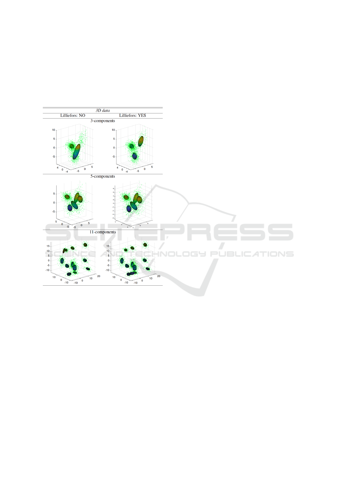
Figure 2: 3D synthetic data segmentation.
Fig. 1 and 2 show the results for the input data
sets together with the original mixtures, both for the
FSAEM-EM original formulation without the Lil-
liefors test, and the herein proposed solution FSAEM-
EM-L. Then, Tab. 1 reports the:
• number of the original mixture components;
• number of detected components;
• number of total iterations;
• difference in % between the number of iterations
without and with the Lilliefors test;
• elapsed time;
• difference in % between the time without and with
the Lilliefors test;
• final log-likelihood;
• normalized L2 distance to the original mixture;
• mean and standard deviation of the differences of
iterations and time.
The best results are in bold, chosen e.g. as the clos-
est number of component or shorter normalized L2
distance with respect to the ground truth mixture, or
fewer iterations, less computational time or higher
loglikelihood). The percentage difference for the time
and the number of iterations has been evaluated with
respect to the values obtained without the Lilliefors
test, so far e.g. (value without test - value with test) /
(value without test) * 100. The usage of the Lilliefors
test gives rise to a remarkable computational improve-
ment, underlined by the large differences in iterations
and computation time.
Without the Lilliefors test, each component is
splitted each time regardless this operation is neces-
sary or not. Predictably, introducing a Gaussianity
test which, if positive, can save some splitting opera-
tions, would result in a reduction of the computational
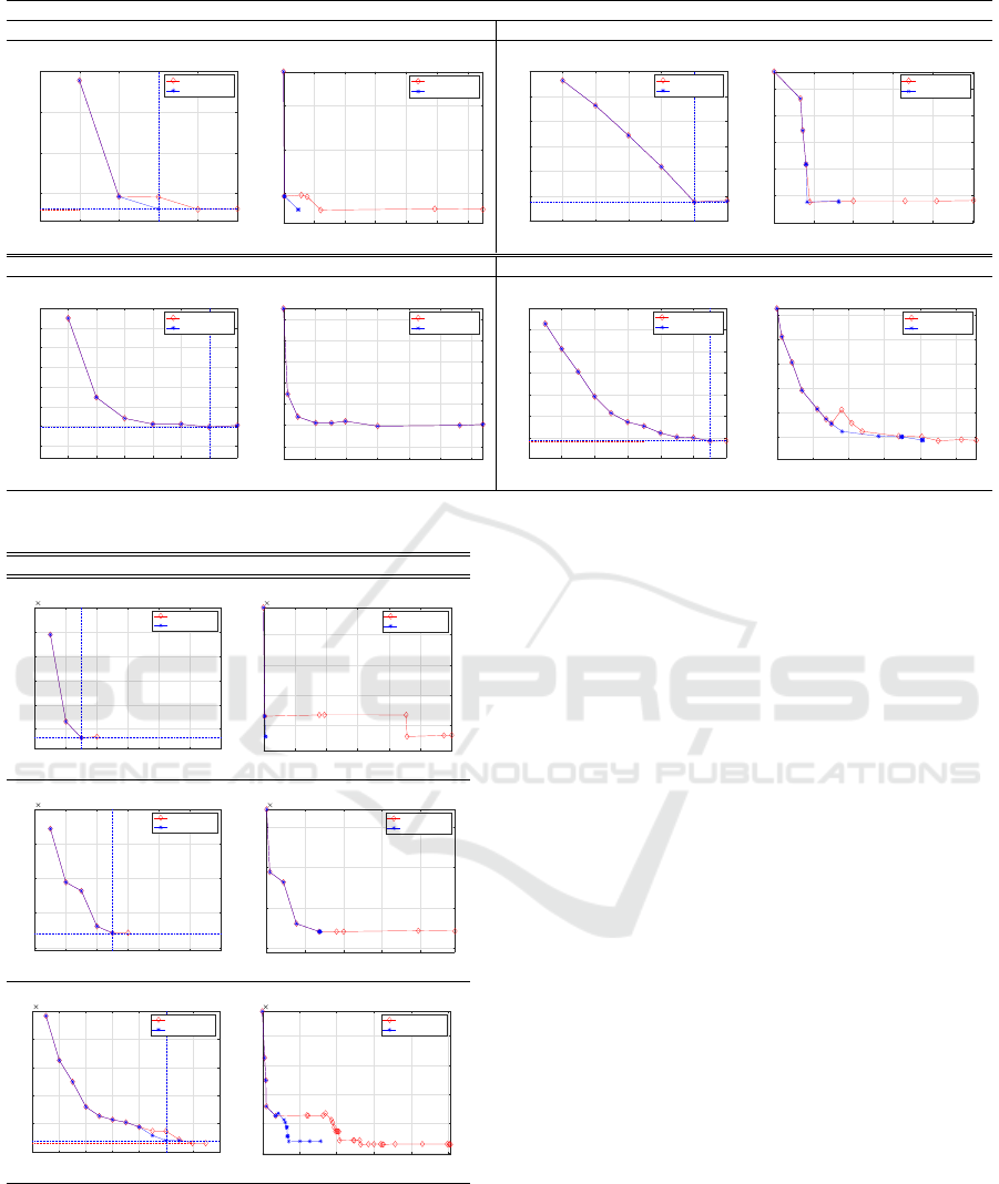
complexity. Fig. 3 and 4 show the evolution of the
cost function vs the number of components and then
vs the number of iterations. Herein it is possible to
observe how the algorithm formulation that includes
the Lilliefors test reaches its optimum faster, i.e. with
less iterations, than the original formulation.
This experiments shows that many operations can
be saved through the Lilliefors test before splitting a
component, bypassing that operation if deemed un-
necessary. This is more evident when the input data
is composed by few components, lowering its effect
when the complexity of mixture grows. This makes
sense also remarking that the computational complex-
ity of the whole EM goes with the dimension of the
input. Moreover, performing a split when not needed,
could even result in a worse local optimum conver-
gence of the EM algorithm, so far bringing about
to a worse final GMM description of the input data.
This is quite evident with the 11 component 3D input,
where the original formulation overfits.
Finally, it is worth noticing that due to space limi-
tations, there are some other issues that cannot be ad-
dressed herein, like the applicability of this algorithm
to other datasets. For these and other inquiries, we
remind to the original work describing FSAEM-EM
Greggio and Bernardino (2024).
4 CONCLUSION
In this paper, we proposed improvements to incre-
mental split based for GMM estimation. These meth-
ods start from a single mixture component and se-
quentially increases the number of components while
Principal Direction 2-Gaussian Fit
315

2D data
3-components 5-components
0 1 2 3 4 5
Number of components
7500
8000
8500
9000
Cost function
Lilliefors: NO
Lilliefors: YES
200 400 600 800 1000 1200
Iterations
7500
8000
8500
Cost function
Lilliefors: NO
Lilliefors: YES
0 1 2 3 4 5 6
Number of components
7600
7800
8000
8200
8400
8600
8800
Cost function
Lilliefors: NO
Lilliefors: YES
1000 2000 3000 4000 5000
Iterations
7600
7800
8000
8200
8400
8600
Cost function
Lilliefors: NO
Lilliefors: YES
6-components 10-components
0 1 2 3 4 5 6 7
Number of components
7800
7900
8000
8100
8200
8300
8400
8500
Cost function
Lilliefors: NO
Lilliefors: YES
500 1000 1500 2000 2500 3000
Iterations
7800
7900
8000
8100
8200
8300
8400
Cost function
Lilliefors: NO
Lilliefors: YES
0 2 4 6 8 10 12
Number of components
7800
8000
8200
8400
8600
8800
9000
Cost function
Lilliefors: NO
Lilliefors: YES
500 1000 1500 2000 2500
Iterations
7800
8000
8200
8400
8600
8800
Cost function
Lilliefors: NO
Lilliefors: YES
Figure 3: 2D synthetic data cost function vs the number of components and then vs the number of iterations.
3D data
3-components
0 2 4 6 8 10 12
Number of components
1.15
1.2
1.25
1.3
1.35
1.4
10
4
Cost function
Lilliefors: NO
Lilliefors: YES
1000 2000 3000 4000 5000 6000
Iterations
1.15
1.2
1.25
1.3
10
4
Cost function
Lilliefors: NO
Lilliefors: YES
5-components
0 2 4 6 8 10 12
Number of components
1.25
1.3
1.35
1.4
1.45
10
4
Cost function
Lilliefors: NO
Lilliefors: YES
200 400 600 800
Iterations
1.25
1.3
1.35
1.4
10
4
Cost function
Lilliefors: NO
Lilliefors: YES
11-components
0 2 4 6 8 10 12 14
Number of components
1.6
1.7
1.8
1.9
2
2.1
10
4
Cost function
Lilliefors: NO
Lilliefors: YES
1000 2000 3000 4000 5000
Iterations
1.6
1.7
1.8
1.9
2
10
4
Cost function
Lilliefors: NO
Lilliefors: YES
Figure 4: 3D synthetic data cost function vs the number of
components and then vs the number of iterations.
adapting their means and covariances to improve the
data fit. The key feature presented in this paper is
the use of a Gaussianity test, the Liliefors test, to pri-
oritize the splitting operations on the dimensions of
the components that most deviate from a Gaussian ap-
proximation. The method produces significant com-
putational savings as illustrated in the experiments
performed with synthetic 2D and 3D data.
ACKNOWLEDGEMENTS
This work was supported by FCT through
LARSyS funding (DOI:10.54499/LA/P/0083/2020,
DOI:10.54499/UIDP/50009/2020,
DOI:10.54499/UIDB/50009/2020), and HAVATAR
project (DOI:10.54499/PTDC/EEI-ROB/1155/2020).
REFERENCES
Ahrendt, P. (2005). The multivariate gaussian
probability distribution. Technical report,
http://www2.imm.dtu.dk/pubdb/p.php?3312.
Comon, P. (1994). Independent component analysis: a new
concept? Signal Processing, Elsevier, 36(3):287–314.
Constantinopoulos, C. and Likas, A. (2007). Unsuper-
vised learning of gaussian mixtures based on varia-
tional component splitting. IEEE Trans. on Neural
Networks, 18(3):745–755.
Dempster, A., Laird, N., and Rubin, D. (1977). Maximum
likelihood estimation from incomplete data via the em
algorithm. J. Royal Statistic Soc., 30(B):1–38.
Fritzke, B. (1995). A growing neural gas network learns
topologies. Adv ances in Neural Inform ation Pro-
cessing Systems 7 (NIPS’94), MIT Press, Cambridge
MA, pages 625–632.
Greggio, N. and Bernardino, A. (2024). Unsupervised in-
ICPRAM 2025 - 14th International Conference on Pattern Recognition Applications and Methods
316

cremental estimation of gaussian mixture models with
1d split moves. Pattern Recognition, 150:110306.
Greggio, N., Bernardino, A., Laschi, C., Dario, P., and
Santos-Victor, J. (2011). Fast estimation of gaussian
mixture models for image segmentation. Machine Vi-
sion and Applications, pages 1–17.
Greggio, N., Bernardino, A., Laschi, C., Santos-Victor, J.,
and Dario, P. (2010). Unsupervised greedy learning
of finite mixture models. In IEEE 22th International
Conference on Tools with Artificial Intelligence (IC-
TAI 2010), Arras, France.
Greggio, N., Bernardino, A., and Santos-Victor, J. (2014).
Efficient greedy estimation of mixture models through
a binary tree search. Robotics and Autonomous Sys-
tems, 62(10):1440–1452.
Hartley, H. (1958). Maximum likelihood estimation from
incomplete data. Biometrics, 14:174–194.
Holmstr
¨
om, J. (2002). Growing neural gas - experiments
with gng, gng with utility and supervised gng.
Huber, M. (2011). Adaptive gaussian mixture filter based
on statistical linearization. Information fusion (FU-
SION), 2011, proceedings of the 14th international
conference on, pages 1–8.
Hyv
¨
arinen, A., Karhunen, J., and Oja, E. (2001). Indepen-
dent component analysis. New York: John Wiley and
Sons, ISBN 978-0-471-40540-5.
Jensen, J. H., Ellis, D., Christensen, M. G., and Jensen,
S. H. (October, 2007). Evaluation distance measures
between gaussian mixture models of mfccs. Proc. Int.
Conf. on Music Info. Retrieval ISMIR-07 Vienna, Aus-
tria, pages 107–108.
Kohonen, T. (1982a). Analysis of a simple self-organizing
process. Biological Cybernetics, 44(2):135–140.
Kohonen, T. (1982b). Self-organizing formation of topolog-
ically correct feature maps. Biological Cybernetics,
43(1):59–69.
Li, J. and Barron, A. (2000). Mixture density estimation.
NIPS, MIT Press, 11.
Lilliefors, H. (1967). On the kolmogorov–smirnov test for
normality with mean and variance unknown. Journal
of the American Statistical Association, 62:399–402.
MacQueen, J. B. (1967). Some methods for classifica-
tion and analysis of multivariate observations. Pro-
ceedings of 5th Berkeley Symposium on Mathematical
Statistics and Probability., pages 281–297.
McLachlan, G. and Bashford, K. (1988). Mixture Models:
Inference and Application to Clustering. New York:
Marcell Dekker.
McLachlan, G. and Peel, D. (2000). Finite Mixture Models.
John Wiley and Sons.
McLachlan, G. and T., K. (1997). The EM Algorithm and
Extensions. New York: John Wiley and Sons.
Richardson, S. and Green, P. (1997). On bayesian analysis
of mixtures with an unknown number of components
(with discussion). J. R. Stat. Soc. Ser., 59:731–792.
Ueda, N., Nakano, R., Ghahramani, Y., and Hiton, G.
(2000). Smem algorithm for mixture models. Neu-
ral Comput, 12(10):2109–2128.
Verbeek, J., Vlassis, N., , and Krose, B. (2003). Efficient
greedy learning of gaussian mixture models. Neural
Computation, 15(2):469–485.
Vlassis, N. and Likas, A. (1999). A kurtosis based dynamic
approach to gaussian mixture modeling. IEEE Trans-
actions on Systems, Man, and Cybernetics, Part A,
Systems and Humans, 29(1999).
Vlassis, N. and Likas, A. (2002). A greedy em algorithm for
gaussian mixture learning. Neural Processing Letters,
15:77–87.
Xu, L. and M., J. (1996). On convergence properties of the
em algorithm for gaussian mixtures. Neural Compu-
tation, 8:129–151.
Zhang, Z., Chen, C., Sun, J., and Chan, K. (2003). Em
algorithms for gaussian mixtures with split-and-merge
operation. Pattern Recognition, 36:1973 – 1983.
Zhao, Q., Hautam
´
’aki, V., K
´
’arkk
´
’ainen, I., and Fr
´
’anti,
P. (2012). Random swap em algorithm for gaus-
sian mixture models. Pattern Recognition Letters,
33(16):2120–2126.
Principal Direction 2-Gaussian Fit
317