Backface Distance Fields: Relaxing Signed Distance Fields

obert B

, Csaba B

alint

and G

abor Valasek

otv

os Lor

and University, Faculty of Informatics, Department of Algorithms and their Applications, Hungary

{rob.ban, csabix, valasek}@inf.elte.hu

Keywords:

Sphere Tracing, Signed Distance Fields, Ray-Surface Intersection, Unbounding Spheres, Safety Volumes.

Abstract:

We propose backface distance functions, an implicit volume representation that improves the convergence rate

of sphere tracing. We employ the closest signed distances to backfacing surface points, introducing a relaxed

representation of signed distance functions. The backface and signed distance functions coincide within the

volume. For external points, we prove that a backface distance-sized step is the largest direction-independent

step along a ray that does not pass through the volume boundary more than once. We show analytic and discrete

realizations of our concept. We present a discrete backface distance ﬁeld generation method to construct exact

and approximate ﬁelds from triangular meshes and procedural implicit scenes. We employ generation-time

processing and correction steps in the discrete case to ensure robust surface visualization in combination with

GPU ﬁltering. We validate the proposed discrete and analytic representations empirically as well by comparing

their performance to basic, relaxed, and enhanced sphere tracing and demonstrate that it generally outperforms

the other methods.

1 INTRODUCTION

Signed distance functions (SDFs) and discrete signed

distance ﬁelds provide versatile means to express and

manipulate shapes of high geometric and topologi-

cal complexity. Moreover, there are efﬁcient means

to directly render SDFs. The most popular itera-

tive algorithm for the latter is Hart’s sphere tracing

(Hart, 1996) that operates on both analytic and dis-

crete signed distance representations. Several vari-

ations have been proposed that improve its perfor-

mance while preserving its robustness (Keinert et al.,

2014; B

alint and Valasek, 2018). These approaches

increase the trace step sizes based on user-provided

hyper-parameters. Their optimal values depend on the

scene and whether the input is analytic or discrete.

Our goal is to incorporate a relaxation into the

signed distance representation itself that increases

step sizes during intersection computations. In

essence, we aim to ﬁnd the SDF analogue of relaxed

cone maps (Policarpo and Oliveira, 2007).

As such, we investigate the problem of robust and

efﬁcient ray-surface intersection computation from a

representational perspective. We deviate from tradi-

tional signed distance descriptions by incorporating

https://orcid.org/0000-0002-8266-7444

https://orcid.org/0000-0002-5609-6449

https://orcid.org/0000-0002-0007-8647

an isotropic relaxation into the representation itself

via using shortest signed distances to backfacing sur-

face points. We refer to these constructs as backface

distance functions (BDF) and discrete backface dis-

tance ﬁelds.

We show that open spheres with such radii ensure

that any ray originating from their center may only

intersect the volume boundaries at most once. More-

over, these semidiameters are optimal sphere trace

step sizes if ray directions are not known a priori. The

BDF coincides with the SDF on the interior of vol-

umes, allowing the sphere trace algorithm to render

discrete and analytic BDFs.

Our main results are summarized as follows:

• We give a geometric and analytic characterization

of backface distance functions and show that these

are complete yet discontinuous volume represen-

tations.

• We derive the analytic BDF for several primi-

tives and show empirically that these can be traced

more efﬁciently than their SDF counterparts.

• We propose a discrete backface distance ﬁeld rep-

resentation that interpolates correctly with GPU

trilinear ﬁltering. It has the same storage require-

ments as a discrete SDF.

• We present a backface distance ﬁeld generation

algorithm that converts signed distance ﬁelds,

Bán, R., Bálint, C. and Valasek, G.

Backface Distance Fields: Relaxing Signed Distance Fields.

DOI: 10.5220/0013251700003912

Paper published under CC license (CC BY-NC-ND 4.0)

In Proceedings of the 20th International Joint Conference on Computer Vision, Imaging and Computer Graphics Theory and Applications (VISIGRAPP 2025) - Volume 1: GRAPP, HUCAPP

and IVAPP, pages 127-138

ISBN: 978-989-758-728-3; ISSN: 2184-4321

127

Figure 1: The three stages of our proposed backface distance ﬁeld (BDF) generation process. First, an input-type dependent

pre-processing step generates data to acquire surface boundary samples throughout the generation process. These samples

may be actual geometric point-normal pairs from the surfaces or auxiliary data that accelerate surface traversals during BDF

computations, such as initial parameter values for closest points for parametric boundaries. The second stage populates a 3D

grid of samples with BDF values in accordance with Algorithm 1. Finally, a correction step, in Algorithm 2, takes this discrete

BDF and expands the SDF region around the zero level set to preserve the original contour and, optionally, surface normals

too. The 256

output BDF of the second stage is rendered at 0.48ms on an Nvidia 2080 GPU at 1920 ×1080 resolution, while

the ﬁnal silhouette- and normal-corrected BDF is rendered at 0.77ms. In comparison, the 256

SDF of the scene is rendered

in 1.02ms on the same conﬁguration.

signed distance functions, general implicits, and

triangular meshes to our proposed representation.

In the following, Section 2 provides an overview

of related work. Our theoretical results are presented

in Section 3, where we provide a geometric and ana-

lytic characterization of the BDF and show that it is

an exact volume representation.

Equipped with these geometric insights, we derive

a simple, GPU-friendly BDF generation algorithm in

Section 4 that is used to convert a variety of represen-

tations into BDFs. We highlight how runtime ﬁltering

footprints must be incorporated into the construction

algorithm to ensure robustness of runtime rendering.

Section 5 presents how ray-surface intersections

are computed on BDFs. In Section 6, we compare

our method to various sphere tracing variants on ana-

lytic and discrete scenes. Finally, we discuss the ad-

vantages and limitations of our technique in Section 7

and conclude our paper.

2 RELATED WORK

2.1 Heightmap Rendering

Our research mainly aimed to identify the SDF equiv-

alent of relaxed cone maps, a data structure used in

heightﬁeld rendering. Heightmaps augment coarser

geometries with mesostructural detail. A wide range

of algorithms have been proposed to compute the per-

pixel exact or approximate ray-heightﬁeld intersec-

tion (Szirmay-Kalos and Umenhoffer, 2008).

To ﬁnd intersections, Dummer proposed to store

the widest upward cone that does not overlap with

the interior of the heightﬁeld (Dummer, 2006). Their

cone step mapping method intersects the rays with

these cones to tend to the exact ray-heightﬁeld inter-

section without skipping intersections.

A relaxation by expanding the cone angles was

proposed in (Policarpo and Oliveira, 2007). The

cones in this representation are the widest that allow

a single intersection between a ray and the height-

ﬁeld if the former is entering the heightﬁeld volume

from above. In contrast to conservative cones, re-

laxed cone maps guide the rays into the heightﬁeld

volume, thus they require a root reﬁnement method,

such as regula falsi, to ﬁnd the precise ray-surface

intersection. Depending on the step counts, relaxed

cone step mapping provides a 5-20% performance im-

provement over conservative cone maps.

In terms of robustness, it must be noted that

relaxed cone maps may skip over intersections for

rays that are already within the heightﬁeld volume.

This issue was investigated in detail by Baboud et

al. in (Baboud et al., 2012) and they resolved it

by proposing an alternative representation that stores

pre-computed safety distances. They also showed the

importance of distances from backfacing triangles in

the computation of the safety distances. More re-

cently, it was shown in (B

an et al., 2024) that nei-

ther conservative nor relaxed cone maps interpolate

correctly under bilinear interpolation, highlighting the

importance of taking into account runtime ﬁltering

during cone map generation.

We set out to derive the SDF analogue to relaxed

cone maps (Policarpo and Oliveira, 2007). We pro-

vide an exact geometric and analytic characterization

of such constructs. We show both analytic and dis-

crete realizations of our proposed representation and

GRAPP 2025 - 20th International Conference on Computer Graphics Theory and Applications

128

verify that similar performance gains can be obtained

to that of relaxed cone maps.

2.2 Signed Distance Representation

Signed distance functions are compact and expres-

sive means to represent and visualize a wide range

of shapes and their various combinations. These are

used in various application domains, from physics,

through geometric modeling, to computer graphics

(Ohtake et al., 2001; Green, 2007; Wright, 2015;

Evans, 2015; Angles et al., 2017; Osher and Fedkiw,

2003; Fuhrmann et al., 2003). As SDFs form a sub-

set of implicit functions, they inherit the property that

unions, intersections, and complements are expressed

as maximum, minimum, and negation operations on

the arguments (Bajaj et al., 1997). However, the re-

sulting functions are generally signed distance lower

bounds, not exact signed distances (Hart, 1996), al-

though alternate set theoretic operation formulations

have been proposed to preserve the distance property

(Akleman and Chen, 2003).

It was noted (Hart, 1996; Kalra and Barr, 1989)

that an SDF value paired with the point of evaluation

deﬁnes an unbounding sphere, an open spherical vol-

ume that does not intersect with the boundaries of the

scene. These are used to traverse a ray at variable step

sizes without skipping over ray-surface intersections.

Keinert et al. (Keinert et al., 2014) proposed a

step-size over-relaxation-based method to speed up

sphere tracing. They use an ω ∈ [1, 2) constant step

size multiplier during trace and fall back to a tradi-

tional sphere trace step if the next guess produces an

unbounding sphere that is disjoint from the previous.

alint et al. (B

alint and Valasek, 2018) reuse data

from the current and previous steps to construct a lin-

ear approximation to the SDF function along the ray

and use it to infer the closest ray parameter where the

unbounding sphere is tangent to the current one. This

is an optimal step size if the approximated surface is

planar. Similarly to the over-relaxation method above,

a basic sphere trace step is taken if the unbounding

sphere is disjoint from the current one.

Galin et al. (Galin et al., 2020) proposed to com-

pute local Lipschitz bounds along the ray, showing

that it could provide more efﬁcient rendering for a

particular family of implicit functions. Their segment

tracing technique offers high accuracy and does not

require a fallback to sphere tracing, as all steps are

safe. However, it does not apply to discrete represen-

tations, it is currently restricted to a subset of implicit

representations, and even though it solves ray-surface

intersection queries in a handful of steps, these it-

erations are costly computationally. Aydinlilar and

Figure 2: Signed distance function (left) and backface dis-

tance function (right) comparison in two dimensions. Three

parallel rays are traced for each representation comparing

how sphere tracing ﬁnds the closest intersection.

Zanni (Aydinlilar and Zanni, 2023) propose to use

bounds on the derivatives to infer conservative upper

and lower bounds on the function value along the ray.

Our proposed representation has both analytic and

discrete realizations. It is rendered by basic sphere

tracing and does not require a hyperparameter. More-

over, we show that it outperforms basic, relaxed, and

enhanced sphere tracing both for analytic and discrete

input. As our representation coincides with SDFs

in volume interiors, it trivially retains the same con-

tour as SDFs, however, this requires a BDF correc-

tion step for the discrete case that we show in Sec-

tion 4. BDFs are closed under union using the same

functional point-wise minimum representation. Un-

like SDF lower bounds, however, it is not closed un-

der intersections and complements.

3 BACKFACE DISTANCE

FUNCTIONS

In this section, we investigate the theoretical proper-

ties of backface distance functions. We present a ge-

ometric and analytic characterization of the boundary

entities that function as the closest surface points for

the BDF distance values. We also show that the BDF

is an exact representation of the volume from which

it was generated; as such, it is not merely an auxil-

iary acceleration structure for rendering but a com-

plete volume representation.

3.1 Notation and SDFs

Let

x =

∥x

x∥

denote the direction of x

x ̸= 0

0. The c ∈ R

level set of an implicit function f

→ R is written

as {f = c} = {x

x ∈ R

| f (x

x) = c}. Similarly, {f ≤

c} = {x

x ∈ R

| f (x

x) ≤ c}. An f

→ R function

Backface Distance Fields: Relaxing Signed Distance Fields

129

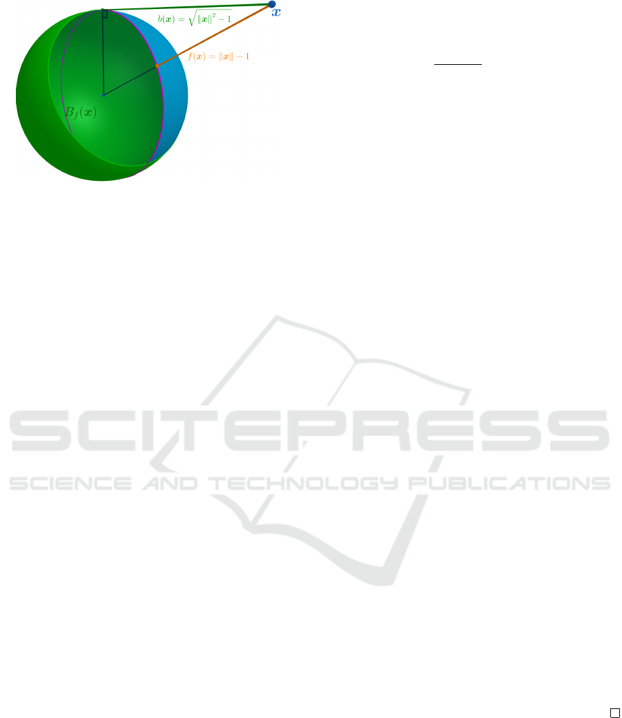
Figure 3: The length of the green line represents the value

of the backface distance function of the unit sphere at point

x, whereas that of the orange segment represents the signed

distance value. The green surface section is the backface

surface set B

x).

is a distance function (DF) if

f (x

x) = d(x

x, {f = 0}) = inf{∥x

x −y

y∥ | f (y

y) = 0},

(1)

and a signed distance function (SDF) if it is continu-

ous and |f | is a distance function (B

alint et al., 2019;

Luo et al., 2019). Usually, we require the SDF to

change sign when crossing the {f = 0} surface for

set operations and normal vector computation. The

term unbounding sphere refers to the |f (x

x)| radius

open ball around x

x ∈ R

, i.e. k

f (x

x) = {y

y ∈ R

∥y

y −x

x∥ < |f (x

x)|}, where f is an SDF.

3.2 BDF Deﬁnition and Geometry

Let us investigate the problem of ﬁnding the maxi-

mal open sphere such that any ray originating from

its center intersects the volume boundaries within the

sphere at most once. Generally, the radius of such a

sphere may be formulated as the signed distance to

the closest backface, i.e., points where the gradient

points away from the center of the sphere. Formally,

this is written as follows.

Deﬁnition 1. Assume that the f

→R SDF is dif-

ferentiable on the {f = 0} surface. The backface sur-

face set B

x) is deﬁned for all x

x ∈R

x) = {y

y ∈ {f = 0} | ∇ f (y

·(y

y −x

x) ≥ 0}. (2)

Deﬁnition 2. Assume that the f

→R SDF is dif-

ferentiable on the {f = 0} surface. The b

→ R

function is a backface distance function (BDF) if

b(x

x) = sgn( f (x

x)) ·d(x

x, B

x)). (3)

Note that this implies that the BDF coincides

with the SDF inside the geometry, that is, for all

x ∈ {f ≤ 0}

b(x

x) = f (x

x) holds. Moreover, since

x) ⊆ {f = 0} for all x

x ∈ R

, the backface dis-

tances are never less than the distance function, mean-

ing



f (x



≤



b(x



. This implies that the zero level-set

is the same, so storing both functions is unnecessary

solely for surface reconstruction. For example, the

BDF of a sphere in Fig. 3 is

sphere

x) =

(

∥x

x∥

−1 if ∥x

x∥ > 1

∥x

x∥−1 if ∥x

x∥ ≤ 1

x ∈R

(4)

For polygons and polyhedrons, we calculate it as

the minimum distance to the backfacing sides. Fig-

ure 2 compares the exact SDF with the BDF.

Note that the BDF is not continuous. For example,

each plane of any small planar surface patch separates

the BDF into discontinuous partitions.

Let us now consider the problem of intersecting

rays with backface distance functions. We show that

taking a |b(x

x)|−ε sized step in any direction from

x may step over at most one root. If the sign of the

function changed after a step, a single root was over-

stepped; and if the sign did not change, no surface

intersection was skipped.

Proposition 1. Assume that the {b = 0} surface is

differentiable, where b

→R is its BDF. Then, for

any x

x + t

v ray, the following equation has at most a

single root in t ∈ [0, b(x

x) −ε] for any ε > 0:

b(x

x +t

v) = 0 (5)

Proof. We can assume that x

x is outside, that is, b(x

x) >

0. First, we show that the set of solutions is at most ﬁ-

nite, and then we prove that it cannot have two differ-

ent elements. If there were a countable or otherwise

inﬁnite number of solutions within that interval, there

would be an accumulation point around t

∗

, and any

neighborhood around it contains an inﬁnite amount

of solutions. Since f is continuous, f (x

x + t

∗

v) = 0.

This means ∇ f (x

x +t

∗

v) exists, and since f is an SDF,

∥∇ f (x

x +t

∗

v)∥ = 1, and this gradient must be perpen-

dicular to the root series around t

∗

. This means that

x +t

∗

v ∈ B

x), which contradicts t

∗

≤ b(x

x) −ε.

Let us assume that there are two neighboring solu-

tions, t

̸= t

. Since f is continuous and its gradient is

non-diminishing, f must change signs from positive

to negative and back. The sign change is the same as

the sign of ∇ f (x

x +t

v, i ∈{1, 2}. Since the signs

differ, one is positive at t

( j ∈ {1, 2}) which would

mean that x

x+t

v ∈B

x). This is a contradiction.

The following observation simpliﬁes the BDF

generation by restricting the minimum distance

search to points either on the silhouette or where the

surface normal points to the opposite direction to the

query position.

Proposition 2. Assuming a differentiable surface, let

x) = {y

y ∈ {f = 0} | ∇ f (y

·(

[

y −x

x) = c}, (6)

GRAPP 2025 - 20th International Conference on Computer Graphics Theory and Applications

130

for any c ∈[−1, 1]. Then, the backface distance func-

tion is

b(x

x) = d



x, B

x) ∪B



. (7)

Proof. Deﬁnition 2 is a conditional minimization

problem on the closed set M = {y

y ∈ {f = 0} |

∇ f (y

·(y

y −x

x) ≥ 0}. Thus, the minimum either lies

on the boundary of M or inside. In the former case,

∂M ∩{f = 0} = B

x). If we omit the condition, we

have a standard closest point problem where we min-

imize ∥y

y −x

x∥ for x

x given that f (y

y) = 0. Applying

the Lagrange multiplier method gives the following

equation for the derivative for some λ ∈ R parameter

∇L(y

y) =

y −x

x) + λ∇ f (y

y) = 0 .

This means that

y −x

x) and ∇ f (y

y) are parallel at

the minimum. Because y

y ∈ M, and f is an SDF

so ∥∇ f (y

y)∥ = 1 where differentiable, thus ∇ f (y

y −x

x) = 1 in this case.

Although the BDF is an SDF in the interior and

on the boundary, it does not automatically inherit its

ease of interoperability with set-theoretic operations.

Let b

, b

→ R be two BDFs. For union, we

can take the pointwise minimum to bound the values

from below via min(b

, b

) = x

x 7→ min(b

x), b

x))

to obtain a BDF of the {b

≤ 0}∪{b

≤ 0} objects.

However, similar results do not hold for intersection,

complement, or subtraction. That is, the maximum of

two BDFs and the negation of a BDF does not yield

a bound on the BDF of the intersection and comple-

ment operations, even though the minimum as a union

operation yields a correct BDF outside.

4 BACKFACE DISTANCE FIELDS

Let us now consider the problem of generating BDF

values for a grid of samples. At runtime, these sam-

ples are ﬁltered to approximate the BDF. We present

a method that converts various representations to dis-

crete backface distance ﬁelds. The algorithm itself is

composed of three stages, as illustrated by Fig. 1: i)

input processing, ii) raw backface distance grid gen-

eration, and iii) backface distance ﬁeld correction.

Input processing is not necessary for all input

types. It generates data that accelerates closest-point

computations via initial points or geometric proxies.

The BDF generation stage outputs a dense 3D grid

of backface distance values. In general, boundary

traversal and determination of the backfacing prop-

erty are input-type dependent. Alternatively, it may

be carried out on the proxy outputs generated in the

input processing step.

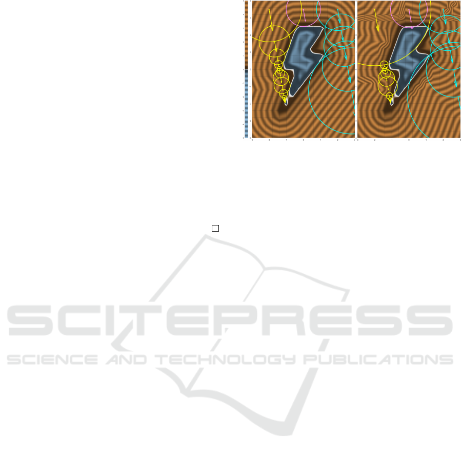
Figure 4: Interpolated SDF (left) and BDF (right) compar-

ison in 2D. The surface and sphere tracing overstep due to

interpolation have been ﬁxed for the BDF.

In the BDF correction stage, the backface dis-

tances are further processed so that interpolation be-

tween samples yields a robustly traceable BDF ap-

proximation.

Since the BDF values can change discontinuously,

the interpolated value of the stored exact samples can

exceed the value of the true analytical BDF at the

evaluation position. This can lead to distance over-

estimation while tracing the interpolated BDF, result-

ing in missing intersections. We solve this problem

by modifying the stored BDF samples such that over-

stepping is prevented using the interpolated values.

We phrase these algorithms in terms of a general

formalism that accommodates a wide variety of input

geometry types. We introduce it next and apply it to

the evaluation of the BDF.

4.1 Evaluating the BDF

The input geometry of the discrete BDF construction

algorithm can be given by general implicit functions,

analytic or discrete SDFs or lower bounds, parametric

surfaces, or triangle meshes. To deal with all these

cases in a concise manner, we introduce the following

notational shorthands.

Let V ⊆ R

denote a volume and ∂V ⊆ R

its

boundary. For any p

p ∈ ∂V , let n

n(p

p) denote an un-

normalized normal vector. Depending on the type of

input geometry, it may be computed as, for example,

n(p

p) =











∇ f (p

p) for an implicit surface

∂

r(u, v) ×∂

r(u, v) for a parametric surface

b −a

a) ×(c

c −a

a) for an a

a, b

b, c

ctriangle

(8)

The evaluation of the BDF at an x

x ∈ R

point is

the solution to

min

∥p

p −x

x∥ | p

p ∈ ∂V, n

n(p

·(p

p −x

x) ≥ 0

(9)

Backface Distance Fields: Relaxing Signed Distance Fields

131

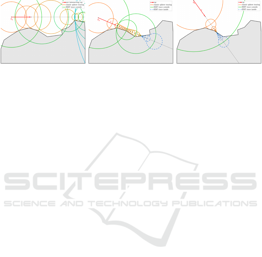
Figure 5: Three cases of tracing the SDF (in red) and the BDF (in green and blue) are displayed. On the left, the ray diverges

to inﬁnity, and our method leaves the frame in half as many steps. On the middle and the right, the ray intersects the surface,

the BDF tracing steps inside and performs sphere tracing backwards to the root, rarely taking more steps (right).

with the sign (−1)

, where χ

x) is the charac-

teristic function of V , i.e. χ

x) = 1 (x

x ∈ V ) and

x) = 0 (x

x ̸∈V ).

4.2 Input Processing

The input processing stage augments the input geom-

etry with data that can be used to accelerate closest

point queries.

For implicit and SDF input, our implementation

generates surface point-normal pairs in this stage, and

these samples replace the input function. This ab-

stracts away the input for the next stage at the expense

of precision. These pairs are stored in a linear buffer.

For triangular meshes, we skip this phase and

compute the exact BDF value at each sample position.

However, additional closest point query acceleration

data may be built here, such as bounding volumes or

space partitioning structures.

For parametric boundaries, this stage can gener-

ate a 3D grid where each sample stores a parametric

patch identiﬁer and the (u, v) parameters of the clos-

est surface point to the sample position. Similarly,

for implicit input, the closest boundary points may be

stored. These can be used as initial guesses in the

next stage of the algorithm when looking for the clos-

est analytic backfaces.

4.3 BDF Grid Computation

Let G ⊆R

denote the set of discrete ﬁeld sample po-

sitions deﬁned on a grid. For example, in a grid with

corner g

∈ R

, sample spacing ∆

, ∆

, and reso-

lution (I + 1) ×(J + 1) ×(K + 1), the grid positions

are

G = {g

+(i∆

, j∆

, k∆

) | i = 0..I, j = 0..J, k = 0..K}.

(10)

Let f [x

x] and b[x

x] denote sample access for dis-

crete signed and backface distance ﬁelds, respec-

tively, where x

x ∈ G is a valid sample position. Our

implementation indexes with (i, j, k) from Eq. (10).

Algorithm 1 is an input-agnostic pseudocode for

generating discrete backface distance ﬁelds. The al-

gorithm calculates the BDF value at each sample po-

sition x

x ∈G.

Inside the object, where f [x

x] ≤ 0, the BDF and

SDF values coincide due to Deﬁnition 2. Outside the

object, we iterate over all surface primitives and ﬁnd

the closest backfacing part. In practice, we compute

the minimum of the squared distances and only apply

the square root once at the end.

For implicit input, the primitives are surface sam-

ples in the form of (p

n) position-normal pairs from

which the distance is ∥x

x − p

p∥. A better distance ap-

proximation may be achieved with a closest point

search starting from this sample (Saye, 2014). The

surface sample is backfacing if the normal vector

points away from the grid position: (p

p −x

n ≥ 0.

We do not necessarily need a discrete SDF to deter-

mine the sign; the original implicit function can be

used instead. If the signed distances are not known

prior to BDF generation, we can calculate the SDF

values alongside the BDF from the same surface sam-

ples.

4.3.1 Mesh Input

For mesh inputs, the triangle distances (Quilez, 2014)

are calculated with Algorithm 4. Face orientation

is determined according to Eq. (8). When a water-

tight mesh is supplied without its SDF, we calculate it

alongside the BDF. Robust methods exist for sign de-

termination (Baerentzen and Aanaes, 2005), yet ray

casting worked well enough for our test cases.

The interpolation problem is partially solved

within this step. During the generation of positive

BDF values, the backfacing condition is relaxed to

ensure that the interpolation is a lower bound where

the exact BDF has discontinuities. To ensure the cor-

rectness of IsBackFacingPrimitive(x

x, s), we have to

check whether the primitive is backfacing from any

point within the cell of x

x. The neighborhood that a

GRAPP 2025 - 20th International Conference on Computer Graphics Theory and Applications

132

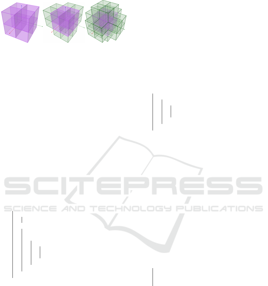
Figure 6: Closest neighbor search kernels for ﬁxing the sur-

face smoothness only (left), for normal calculation with the

forward difference (middle), and for correct normal calcu-

lation with symmetric difference method (right).

grid sample inﬂuences during interpolation is

−∆

, x

+∆

]×[x

−∆

, x

+∆

]×[x

−∆

, x

+∆

(11)

The backfacing condition for the box is simpliﬁed to

checking the farthest cell corner from the plane of the

normal:

c = x

x −(sgn(

)∆

, sgn(

)∆

, sgn(

)∆

). (12)

Then IsBackFacingPrimitive(x

x, s) = (p

p −c

n ≥ 0.

Our BDF generation is implemented in compute

shaders that execute in parallel for each sample on the

GPU. Depending on the input size, the BDF genera-

tion is subdivided into several batches for better com-

puting efﬁciency. If needed, the consecutive batches

store the intermediate squared minimum distances.

Data: G ⊆R

set of grid positions, f

G →R

SDF, S set of surface primitives

Result: b

G →R backface distance ﬁeld

forall x

x ∈G sample position do

if f [x

x] ≤ 0 then

b[x

x] ← f [x

x];

else

b[x

x] ← +∞ ;

forall s ∈S surface primitive do

if IsBackFacingPrimitive(x

x, s) then

d ← DistanceToPrimitive(x

x, s);

b[x

x] ← min(b[x

x], d);

end

Algorithm 1: Calculating discrete BDFs (stage 2).

4.4 BDF Correction

The ﬁnal stage of discrete BDF generation ensures

correct interpolation near the surface. As the true

analytical BDF can have discontinuities or singular-

ities along the surface, the interpolated surface will

be offset and exhibit wrinkles and artifacts along cell

boundaries. The surface is corrected by replacing the

stored larger BDF values with SDF values near the

surface. In Algorithm 2, we replace the stored val-

ues if any of its neighbors are negative. The shapes

and sizes of this neighborhood kernel are visualized

in Fig. 6. When high-quality surface normals are not

required, we may correct within the smallest neigh-

borhood to retain more performance of the BDF. Sur-

face normal calculations rely on numeric differentials

that may become faulty on cell boundaries when the

next cell contains much larger BDF values. We have

to use a larger search kernel for the correct symmetric

and one-sided differentials.

Data: G ⊆R

set of grid positions, f

G →R

SDF, b

G →R backface distance ﬁeld

Result: b

G →R modiﬁed BDF

forall x

x ∈G sample position do

forall y

y ∈NeighbourSamples(x

x) do

if f [y

y] ≤ 0 then

b[x

x] ← f [x

x];

break;

end

Algorithm 2: Correcting discrete BDFs (stage 3).

5 RENDERING BACKFACE

REPRESENTATIONS

The common advantage of analytic and discrete back-

face distance representations is the simplicity of the

rendering algorithm: the sphere tracing algorithm,

listed in Algorithm 3. Since a BDF-sized step may

leap into the volume, the trace then starts going back-

ward via negative stepsizes in a basic sphere tracing

fashion as in Fig. 5.

Data: p

v ray, b

→ R BDF

Result: t ≥ 0 distance traveled to the ﬁrst

intersection

t ← 0; i ←0;

repeat

r ← b(p

v);

t ←t + r;

i ←i + 1;

until

< ε or t ≥t

max

or i ≥i

max

;

Algorithm 3: Sphere tracing a BDF.

Due to the interpolation error in the discrete case,

the sphere trace on the inferred SDF might step out-

side once again; however, the interpolation error is

smaller than the cell size. This means that the cor-

rected BDF in that cell equals the SDF and will con-

verge to the trilinear surface. While sphere tracing us-

ing SDFs ﬁnds the solution without ever allowing the

tracing to enter the volume, tracing with BDFs often

guides the steps inside the volume and simultaneously

ﬂips the tracing direction. Sphere tracing of the two

Backface Distance Fields: Relaxing Signed Distance Fields

133

Figure 7: Procedural scenes used in our analytic BDF performance tests, including blobs and various primitives.

representations is compared in Fig. 2 for the analytic

case and in Fig. 4 for a 2D discrete BDF ﬁeld.

Experimental algorithms that explicitly split the

loop into two phases, one for exterior and one for

internal trace, proved to be much slower. Even if

we employ root-ﬁnding methods upon the ﬁrst sign

change, such as bisection or regula-falsi, the per-

formance is lower than the sphere tracing algorithm

above.

A slight modiﬁcation to the tracing algorithm al-

lows for faster shadow calculation. Since the BDF

guarantees that a sphere tracing step only skips at

most one intersection point, we can stop tracing at

the ﬁrst sign change. In practice, this means stopping

when r < ε instead of |r| < ε in Algorithm 3.

6 TEST RESULTS

We tested our proposed analytic and discrete BDF

representations in rendering scenarios, and compared

performance statistics to basic (Hart, 1996), relaxed

(Keinert et al., 2014), and enhanced sphere tracing

alint and Valasek, 2018), adapting the nomencla-

ture from the latter. Algorithm 3 was used for BDF

rendering. We manually selected a relaxation param-

eter ω = 1.6 for relaxed sphere tracing and ω = 0.88

for enhanced sphere tracing, providing the best speed-

up while retaining geometric accuracy.

We implemented the tracing and generation meth-

ods in the NVIDIA Falcor (Kallweit et al., 2022)

framework in C++ with DirectX 12 backend. We

ran tests on triangular meshes and procedural scenes

adapted from (Takikawa et al., 2022). Measurements

were taken with both AMD and NVIDIA GPUs in a

resolution of 1920 ×1080. The distance ﬁelds were

stored in 16-bit half-precision 3D textures. The full

implementation will be released.

6.1 BDF Correction

The samples in a discrete BDF differ from simple

backface distance function evaluations, as shown in

Section 4.3 and Section 4.4 These are necessary be-

cause a raw, unprocessed discrete BDF with runtime

trilinear ﬁltering results in blocky renders, such as

shown in Fig. 1. However, these processing steps also

affect real-time performance considerably.

For the bunny mesh, the processed ﬁeld was 24%

and 53% slower at 32 and 1000 iterations than the

raw BDF, respectively. The same correction-induced

performance loss ratios for the M

obius strip amounted

to an average of 19% and 41% on Nvidia 2080 and

16% and 35% on AMD RX 5700.

6.2 Performance of Analytic BDFs

Table 1 summarizes our performance measurements

on procedural scenes, shown in Fig. 7. The derivation

and implementation of BDF functions are located in

our Appendix.

Overall, BDF primitives offered minor to modest

performance improvements over their SDF counter-

parts in 85% of our tests. Shadow rays traced the same

type of procedural geometry as the primary traces.

This made BDFs even more efﬁcient in scenes involv-

ing shadows, as our representation guides rays into

the volumes. A distinct exception was the Box scene

which shows the need for a more efﬁcient BDF ap-

proximation to the box primitive. On the other scenes,

BDFs were 7% and 11% more performant on AMD

and Nvidia than SDFs on average using shadows.

We compared the performance of BDF tracing to

Lipschitz segment tracing (Galin et al., 2020) on a

scene adapted from the authors’ ShaderToy sample.

On AMD RX 5700, Lipschitz segment tracing re-

quired 45% of the frame time of sphere tracing while

our method only needed 38%. Lipschitz and BDF

numbers on the Nvidia 2080 GPU are 48% and 40%,

respectively, showing that BDF tracing outperforms

Lipschitz segment tracing on SDF-like implicit func-

tions.

6.3 Performance of Discrete BDFs

First, we measured the render time performance im-

plications of different ﬁeld sizes, ranging from 64

to 512

. On the highest resolution, discrete BDFs

are unequivocally more efﬁcient (13-25% on average,

in some cases up to 35%) than basic sphere tracing;

however, the dilation of the SDF area to preserve con-

tours and shading normals severely hinders them at

smaller ﬁelds. Consequently, BDF gains are more

GRAPP 2025 - 20th International Conference on Computer Graphics Theory and Applications

134

Table 1: Performance comparison of sphere tracing on procedural signed and backface distance functions (SDF and BDF

columns) with and without hard shadows. Shadow rays are traced on the same representation as the primary rays. Timings on

the SDFs are reported in milliseconds, BDF numbers are relative to sphere tracing, and the resolution was 1920 ×1080.

Box Cylinder Primitives Sphere Torus

GPU Shadow SDF BDF SDF BDF SDF BDF SDF BDF SDF BDF

AMD RX 5700 ON 1.517 135% 1.66 99% 3.155 96% 1.285 83% 1.614 93%

OFF 0.683 142% 0.72 110% 1.345 101% 0.555 91% 0.694 96%

NVIDIA 2080 ON 0.93 133% 1.15 83% 1.66 88% 1.07 87% 1.62 97%

OFF 0.4 130% 0.53 96% 0.75 89% 0.38 87% 0.47 81%

Table 2: Frame render times for NVIDIA 2080 Super for three procedural and two triangular mesh scenes with or without

shadows for sphere tracing (ST), relaxed sphere trace (RT) (Keinert et al., 2014), enhanced sphere tracing (ET) (B

alint and

Valasek, 2018), and our BDF sphere trace method. Sphere tracing runtimes are in milliseconds, the others are relative to those.

Shadows: off Shadows: on

Scene Steps ST RT ET BDF ST RT ET BDF

Spheres 32 0.43 105% 109% 86% 0.66 105% 114% 85%

1000 0.77 92% 93% 77% 1.14 87% 89% 75%

Gears 32 0.28 104% 104% 89% 0.39 103% 105% 87%

1000 0.37 92% 89% 86% 0.5 90% 90% 84%

Mountain 32 0.36 100% 106% 78% 0.55 93% 104% 75%

1000 0.49 86% 96% 71% 0.67 84% 96% 72%

Bunny mesh 32 0.25 100% 100% 88% 0.33 101% 102% 86%

1000 0.32 92% 86% 86% 0.39 92% 90% 85%

Skull mesh 32 0.23 104% 104% 91% 0.31 106% 106% 90%

1000 0.45 84% 82% 89% 0.51 88% 94% 90%

modest (7-11%) at the smallest resolutions.

For the performance comparison between ba-

sic, enhanced, relaxed, and BDF sphere tracing, we

choose the resolution of 128

. We computed exact

BDF ﬁelds for mesh inputs and approximate ones for

procedural SDFs. BDF generation times at this res-

olution were between 0.5-80 seconds on both GPUs,

depending on the input geometry. For meshes, SDF

and BDF generation times were effectively identi-

cal. The measurements in Table 2 were taken at

1920 ×1080 resolution. We recorded timings at low

(32) and high (1000) iteration limits.

BDFs performed signiﬁcantly better on ﬁelds gen-

erated from procedural inputs (19% and 22% faster on

average than sphere tracing with and without shad-

ows on both AMD RX 5700 and Nvidia 2080 Su-

per, respectively) compared to mesh inputs (9% and

12% faster with and without shadows on the AMD

GPU, 12% for both on the Nvidia card). At high iter-

ation counts, relaxed and enhanced sphere tracing ap-

proached or occasionally outperformed BDF traces,

the latter occurring 3.125% of the times in our tests.

The tests showed that high-resolution ﬁelds mask

the performance implications of dilating the SDF re-

gion within the discrete BDFs. This is explained by

the smaller absolute volumes on which the SDF is re-

instated. Even with our representation, the silhouettes

are hotspots for iterations, but much less so.

However, note that performance also drops due

to the more conservative backface selection property

that takes into account the ﬁltering footprint when

selecting prospective backfaces. Further research is

needed to identify if the gap between raw and cor-

rected discrete BDFs can be narrowed by different

processing at generation time or by other ﬁltering

techniques beyond trilinear at runtime.

7 CONCLUSIONS

We proposed a new volumetric representation, back-

face distance functions. These constructs compute

the signed distances to the closest backfaces and ef-

ﬁciently resolve ray-surface intersections.

We investigated the mathematical properties of

backface distance functions and proved that they pro-

vide a complete geometric description of the scene

without any additional data. We presented procedu-

ral backface distance functions for various primitives

and derived a discrete realization that takes ﬁltering

into account.

We proposed a three-stage algorithm to gener-

ate exact and approximate discrete backface distance

ﬁelds from triangular mesh and procedural implicit

inputs. The main contribution here is how we pre-

Backface Distance Fields: Relaxing Signed Distance Fields

135

serve the same silhouette and shading normal as a dis-

crete signed distance ﬁeld via additional processing

steps.

Our performance tests showed that tracing on our

analytic and discrete representations is more efﬁcient

than various trace methods on signed distance func-

tions and ﬁelds. Our representation is almost matched

or slightly outperformed by the other algorithms at

very high iteration count limits for a limited set of

inputs. However, this also shows that the shape-

preservation steps hinder the acceleration potential of

backface distance ﬁelds. We veriﬁed this with mea-

surements that up to 41% performance gain is lost

compared to raw backface distance ﬁelds. Neverthe-

less, in general, tracing on our representation con-

verges faster initially, requiring fewer iterations than

the other methods.

Further research is required to mitigate the perfor-

mance loss due to discrete backface distance ﬁeld cor-

rection, either via generation-time processing or run-

time ﬁltering. Similarly, procedural backface distance

function approximations to the results of intersection

and complement set-theoretic operations are subject

to future work.

REFERENCES

Akleman, E. and Chen, J. (2003). Constant Time Update-

able Operations for Implicit Shape Modeling.

Angles, B., Tarini, M., Wyvill, B., Barthe, L., and

Tagliasacchi, A. (2017). Sketch-based Implicit Blend-

ing. ACM Transactions on Graphics, 36(6):1–13.

Aydinlilar, M. and Zanni, C. (2023). Forward inclusion

functions for ray-tracing implicit surfaces. Comput-

ers & Graphics, 114:190–200.

Baboud, L., Eisemann, E., and Seidel, H.-P. (2012). Pre-

computed Safety Shapes for Efﬁcient and Accurate

Height-Field Rendering. IEEE Transactions on Visu-

alization and Computer Graphics, 18(11):1811–1823.

Baerentzen, J. and Aanaes, H. (2005). Signed Distance

Computation Using the Angle Weighted Pseudonor-

mal. IEEE Transactions on Visualization and Com-

puter Graphics, 11(3):243–253.

Bajaj, C., Blinn, J., Cani, M.-P., Rockwood, A., Wyvill, B.,

and Wyvill, G. (1997). Introduction to Implicit Sur-

faces. Morgan Kaufmann Publishers Inc., San Fran-

cisco, CA, USA.

alint, C. and Valasek, G. (2018). Accelerating Sphere

Tracing. In EG 2018 - Short Papers, page 4 pages,

Delft, Netherlands. The Eurographics Association.

alint, C., Valasek, G., and Gerg

o, L. (2019). Opera-

tions on Signed Distance Functions. Acta Cybernet-

ica, 24(1):17–28.

an, R., Valasek, G., B

alint, C., and Vad, V. A. (2024). Ro-

bust cone step mapping. In Haines, E. and Garces, E.,

editors, Eurographics symposium on rendering. The

Eurographics Association. ISSN: 1727-3463.

Dummer, J. (2006). Cone Step Mapping: An Iterative Ray-

Heightﬁeld Intersection Algorithm.

Evans, A. (2015). Learning from Failure: a Survey of

Promising, Unconventional and Mostly Abandoned

Renderers for ’Dreams PS4’, a Geometrically Dense,

Painterly UGC Game. In Advances in Real-Time Ren-

dering in Games. SIGGRAPH, MediaMolecule.

Fuhrmann, A., Sobotka, G., and Groß, C. (2003). Distance

ﬁelds for rapid collision detection in physically based

modeling. International Conference Graphicon 2003.

Galin, E., Gu

erin, E., Paris, A., and Peytavie, A. (2020).

Segment Tracing Using Local Lipschitz Bounds.

Computer Graphics Forum, 39(2):545–554.

Green, C. (2007). Improved Alpha-tested Magniﬁcation

for Vector Textures and Special Effects. In ACM

SIGGRAPH 2007 courses on - SIGGRAPH ’07, SIG-

GRAPH ’07, pages 9–18, San Diego, California.

ACM Press.

Hart, J. C. (1996). Sphere Tracing: A Geometric Method

for the Antialiased Ray Tracing of Implicit Surfaces.

The Visual Computer, 12(10):527–545.

Kallweit, S., Clarberg, P., Kolb, C., Davidovi

c, T., Yao,

K.-H., Foley, T., He, Y., Wu, L., Chen, L., Akenine-

oller, T., Wyman, C., Crassin, C., and Benty, N.

(2022). The Falcor Rendering Framework.

Kalra, D. and Barr, A. H. (1989). Guaranteed Ray Inter-

sections with Implicit Surfaces. In 16th Annual Con-

ference on Computer Graphics and Interactive Tech-

niques, SIGGRAPH ’89, pages 297–306, New York,

NY, USA. Association for Computing Machinery.

Keinert, B., Sch

afer, H., Kornd

orfer, J., Ganse, U., and

Stamminger, M. (2014). Enhanced Sphere Tracing.

In Smart Tools and Apps for Graphics - Eurographics

Italian Chapter Conference, page 8 pages. The Euro-

graphics Association.

Luo, H., Wang, X., and Lukens, B. (2019). Variational

Analysis on the Signed Distance Functions. Journal of

Optimization Theory and Applications, 180(3):751–

774.

Ohtake, Y., Belyaev, A., and Pasko, A. (2001). Dynamic

meshes for accurate polygonization of implicit sur-

faces with sharp features. In International Conference

on Shape Modeling and Applications, pages 74–81,

Genova, Italy. IEEE Computer Society.

Osher, S. and Fedkiw, R. (2003). Signed Distance Func-

tions. In Antman, S. S., Marsden, J. E., and Sirovich,

L., editors, Level Set Methods and Dynamic Implicit

Surfaces, volume 153, pages 17–22. Springer New

York, New York, NY. Series Title: Applied Mathe-

matical Sciences.

Policarpo, F. and Oliveira, M. M. (2007). Relaxed Cone

Stepping for Relief Mapping. In GPU Gems 3.

Quilez, I. (2014). Distance to a Triangle.

Saye, R. (2014). High-order methods for computing dis-

tances to implicitly deﬁned surfaces. Communications

in Applied Mathematics and Computational Science,

9(1):107–141.

GRAPP 2025 - 20th International Conference on Computer Graphics Theory and Applications

136

Szirmay-Kalos, L. and Umenhoffer, T. (2008). Displace-

ment Mapping on the GPU - State of the Art. Com-

puter Graphics Forum, 27(6):1567–1592.

Takikawa, T., Glassner, A., and McGuire, M. (2022). A

Dataset and Explorer for 3D Signed Distance Func-

tions. Journal of Computer Graphics Techniques

(JCGT), 11(2):1–29.

Wright, D. (2015). Dynamic Occlusion with Signed Dis-

tance Fields. Epic Games (Unreal Engine).

APPENDIX

Analytic Backface Distance Functions

In this section, we list some of the analytic backface

distance primitives along with their SDF counterparts

when evaluating at an x

x = [x, y, z]

query point.

Unit Sphere

We have to calculate the length of a segment tangen-

tial to the sphere from the x

x query point.

SDF: f (x

x) = ∥x

x∥−1

BDF: b(x

x) =

(

∥x

x∥

−1 if f (x

x) > 0

f (x

x) if f (x

x) ≤ 0

The difference between the BDF and the SDF for the

sphere is

sphere

x) − f

sphere

x) =

∥x

x∥

−1 −∥x

x∥+ 1,

where ∥x

x∥ > 1. This difference approaches 1 as

∥x

x∥ → ∞. In practice, tracing a BDF takes larger

steps by the sphere radius but slows down near the

surface because of local concavity. However, the

slowdown near the surface is much smaller because

lim

∥x

x∥→0

b(x

f (x

= +∞.

Inﬁnite Cylinder

The equation for the cylinder is the same, except that

it only needs two dimensions.

(a) Finite cylinder (b) Torus

Figure 8: Geometry of the BDF and its construction for the

two primitives. The green surface on the ﬁnite cylinder is

the backface surface set B

x) as seen from query point x

SDF: f (x, y, z) =

+ y

−1

BDF: b(x, y, z) =

(

+ y

−1 if f (x, y, z) > 0

f (x, y, z) if f (x, y, z) ≤ 0

The formula for the ﬁnite cylinder is more involved.

Figure 8a aids with interpreting the source code.

Inﬁnite Cone

The cone is similar to the cylinder, the radius changes

with the z coordinate. From now on, we always as-

sume that b(x, y, z) = f (x, y, z) when f (x, y, z) < 0, so

we only list when f (x, y, z) > 0.

SDF: f (x, y, z) =

√

−ztan α

1+tan

BDF: b(x, y, z) =

+ y

−(z tan α)

Torus

The BDF of the torus is visualized in Fig. 8b.

SDF: f (x, y, z) =



+ y

−R



+ z

−r

BDF: b(x, y, z) =



+ y

−R



+ z

−r

Data: G ⊆ R

set of grid positions, and T set of

triangles, d

r = [1, 0, 0]

arbitrary direction

for sign determination

Result: f

G →R signed distance ﬁeld, and

G →R backface distance ﬁeld

forall x

x ∈G sample position do

b2 ←+∞;

f 2 ← +∞;

sign ←1;

forall t ∈ T triangle do

d2 ←SquaredDistanceToTriangle(x

x,t);

f 2 ← min( f 2, d2) ;

if IntersectTriangle(x

x, d

r, t) then

sign ←−sign ;

end

if IsBackFacingTriangle(x

x,t) then

b2 ←min(b2, d2) ;

end

f [x

x] ← sign ·

√

f 2;

b[x

x] ← sign ·

√

b2;

end

Algorithm 4: Calculating SDF and BDF for a mesh.

Plane

The BDF values of a plane with unit normal

n ∈ R

are inﬁnite throughout the whole positive half-space

because the surface has no backfaces viewed from

there. We rectify this by setting an arbitrary value in

Backface Distance Fields: Relaxing Signed Distance Fields

137

(a) SDF. (b) Non-conservative BDF. (c) Conservative BDF.

Figure 9: Comparison of baseline SDF (left) to post-processed but non-conservatively (center) and conservatively (right)

generated 128

BDFs.

the following shader code to allow the sphere tracing

to trace backward from there. Due to the sphere trac-

ing slowdown near the surface, this change is actually

much faster than the regular SDF plane, especially if

the horizon is in view.

SDF: f (x

x) = x

BDF: b(x

x) =



+∞ if f (x

x) > 0

f (x

x) if f (x

x) ≤ 0

Data: c

c ∈R

starting grid corner, (I, J, K) ∈ N

grid resolution, ∆ ∈ R

grid spacing,

→ R SDF, ρ ∈ (0, 1] search step

relaxation

Result: S ⊆ R

×R

set of position-normal pairs

(surface samples)

S ←

forall p

p ∈{c

c + ∆ ·[i, j, k]

|0 ≤ i < I, 0 ≤ j <

J, 0 ≤k < K} do

if |f (p

p)| ≤

√

3 ·∆ then

q ← p

p; m = 0 ;

while |f (q

q)| > ε ∧m < m

max

q ←q

q −ρ · f (q

q) ·∇ f (q

q);

m ←m + 1;

end

S ←S ∪



q, ∇ f (q



;

end

Algorithm 5: Surface sample generation from SDF.

General Construction Algorithm

Algorithm 4 calculates both the SDF and the BDF

from a mesh, while Algorithms 5 and 6 generates

BDF from SDF through surface samples. In practice,

the visual difference is negligible between the SDF

and the corrected BDF because both use the same

tracing algorithm as demonstrated on Fig. 9.

BDF Tracing Variant

In practice, we often employ the robust variant of

BDF sphere tracing seen in Algorithm 3. In addition

to the usual termination condition, this method also

Data: G ⊆ R

set of grid positions, f

G →R

SDF, S ⊆ R

×R

set of surface samples

Result: b

G →R backface distance ﬁeld

forall x

x ∈G sample position do

if f [x

x] ≤ 0 then

b[x

x] ← f [x

x];

else

b2 ←+∞ ;

forall (p

p, n

n) ∈ S position-normal pair do

if IsBackFacingSample(x

x, p

p, n

n) then

d2 ←∥p

p −x

x∥

;

b2 ←min(b2, d2) ;

end

b[x

x] ←

√

b2;

end

Algorithm 6: Calculating BDF for an SDF.

terminates when the BDF changes sign during the

backward sphere tracing. The advantage is that this

method converges even if the BDF was not corrected.

The BDF texture lookup completely hides the time

it takes to evaluate the additional condition, thus the

render times for the two variants were exactly equal.

GRAPP 2025 - 20th International Conference on Computer Graphics Theory and Applications

138