Evaluating Combinations of Optimizers and Loss Functions for Cloud
Removal Using Diffusion Models
Leandro Henrique Furtado Pinto Silva
1,2
, Jo
˜
ao Fernando Mari
1
, Mauricio C. Escarpinati
2
and Andr
´
e R. Backes
3
1
Institute of Exact and Technological Sciences, Federal University of Vic¸osa - UFV, Rio Parana
´
ıba-MG, Brazil
2
School of Computer Science, Federal University of Uberl
ˆ
andia, Uberl
ˆ
andia, Brazil
3
Department of Computing, Federal University of S
˜
ao Carlos, S
˜
ao Carlos-SP, Brazil
Keywords:
Cloud Removal, Diffusion Model, Remote Sensing, Optimizers, Loss Functions.
Abstract:
Cloud removal is crucial for photogrammetry applications, including urban planning, precision agriculture,
and climate monitoring. Recently, generative models, especially those based on latent diffusion, have shown
remarkable results in high-quality synthetic image generation, making them suitable for cloud removal tasks.
These approaches require optimizing numerous trainable parameters with various optimizers and loss func-
tions. This study evaluates the impact of combining three optimizers (SGD, Adam, and AdamW) with the
MAE, MSE, and Huber loss functions. For evaluation, we used the SEN MTC New dataset, which contains
pairs of 4-band images with and without clouds, divided into training, validation, and test sets. The results,
measured in terms of PSNR and SSIM, show that the diffusion model combining AdamW and the Huber loss
function delivers exceptional performance in cloud removal.
1 INTRODUCTION
Remote sensing, particularly through satellite im-
agery, is vital for environmental monitoring, urban
planning, and precision agriculture. However, these
applications are significantly hindered by cloud pres-
ence, as clouds can obscure areas of interest, af-
fecting measurement accuracy (Jeppesen et al., 2019;
Arakaki et al., 2023; Ferreira et al., 2024). This is-
sue is especially impactful given that clouds with var-
ious characteristics cover approximately 60% of the
Earth’s surface and continuously shift across regions.
Consequently, cloud removal techniques to reduce
these artifacts have gained prominence in recent re-
search (Xie et al., 2023; Podsiadlo et al., 2020).
To address cloud removal, researchers have em-
ployed various approaches, including Convolutional
Neural Networks (CNNs), Generative Adversarial
Networks (GANs), and, more recently, Diffusion
Models (Dong et al., 2021). Although each method
has unique attributes, they are united by their re-
liance on deep learning, and tuning these models of-
ten involves empirical considerations (Barbosa et al.,
2024). Choosing the right optimizers and loss func-
tions is essential to improving the learning process
by accurately updating model weights, which sup-
ports better generalization (Seyrek and Uysal, 2024).
Notably, while optimizer and loss function choices
are crucial for traditional Convolutional Neural Net-
works, these elements require further investigation for
emerging techniques like latent diffusion models.
Through analysis of nine experiments, this study
examines which combinations of optimizers and loss
functions yield optimal results for cloud removal. Our
investigation focuses on the performance impact of
these combinations in diffusion models for cloud re-
moval tasks.
The remaining of this work is organized as fol-
lows: Section 2 presents related works, providing def-
initions that support and motivate this study. Section
3 details the Materials and Methods, including the
experimental setup, dataset, and evaluation metrics.
Section 4 presents the quantitative and qualitative re-
sults and discussions. Finally, Section 5 presents the
conclusions, perspectives of this research, and future
works.
2 RELATED WORKS
The work by Zhao and Jia (2023) introduces a
sequence-based diffusion model for generating cloud-
648
Silva, L. H. F. P., Mari, J. F., Escarpinati, M. C. and Backes, A. R.
Evaluating Combinations of Optimizers and Loss Functions for Cloud Removal Using Diffusion Models.
DOI: 10.5220/0013252100003912
Paper published under CC license (CC BY-NC-ND 4.0)
In Proceedings of the 20th International Joint Conference on Computer Vision, Imaging and Computer Graphics Theory and Applications (VISIGRAPP 2025) - Volume 3: VISAPP, pages
648-656
ISBN: 978-989-758-728-3; ISSN: 2184-4321
Proceedings Copyright © 2025 by SCITEPRESS – Science and Technology Publications, Lda.

free images. This model employs multimodal diffu-
sion for training and sequential inference, integrating
multi-temporal information in a time-invariant man-
ner. Experiments conducted on the four bands of the
public SEN12MS-CR-TS dataset demonstrated that
this model outperforms other approaches in the lit-
erature, highlighting its flexibility in processing se-
quences of arbitrary length.
Zhao et al. (2023) propose a CNN-based method
that takes advantage of radio frequency signals in
the ultra-high and super-high frequency bands, allow-
ing it to “see” through clouds to assist in image re-
construction. This innovative multimodal and multi-
temporal approach demonstrated effectiveness in pro-
ducing cloud-free images in experiments with public
satellite data.
Ebel et al. (2023) present UnCRtainTS, a mul-
titemporal cloud removal method that combines
attention-based features with specialized architec-
tures to predict multivariate uncertainties. Experi-
ments conducted on two public datasets showed this
approach’s high effectiveness in reconstructing im-
ages obscured by clouds.
The study by Wang et al. (2023) introduces a
cloud removal algorithm based on (i) time-series ref-
erence imagery, (ii) selection of similar pixels through
weighted temporal and spectral distances, and (iii)
residual image estimation. The algorithm creates two
“buffer zones” around clouded areas, enabling auto-
matic selection of an “optimal” set of time-series ref-
erence images. Experiments across four diverse lo-
cations, such as urban, rural, and humid areas, which
demonstrated the model’s quantitative effectiveness,
adaptability to varying cloud sizes, and superior per-
formance compared to other methods, with efficient
computational time that makes it suitable for large
datasets.
3 MATERIAL AND METHODS
3.1 Image Dataset
For our experiments, we used the multitemporal
SEN2 MTC New dataset, a heterogeneous collection
of images from various Earth regions (Huang and Wu,
2022). This dataset consists of 50 tiles, each divided
into 256×256 patches across four bands: Red, Green,
Blue, and Near Infrared, including both thin and thick
cloud coverage. Areas with thin clouds contain more
land information, which is crucial for the reconstruc-
tion process; however, thin clouds pose challenges in
cloud segmentation, potentially impacting cloud re-
moval accuracy. In contrast, thick clouds simplify
segmentation, but the land information is more lim-
ited in these images.
The dataset contains 2, 380 image patches for
training, 350 for validation, and 687 for testing, with
each patch containing pairs of cloud-covered images
and their corresponding cloud-free counterparts. For
our experiments, we considered the same quantity as
the original dataset. Figure 1 shows samples of the
patches in the dataset.
3.2 DiffCR
Zou et al. (2024) introduced DiffCR, a diffusion
model for cloud removal that generates Gaussian
noise from cloud-free images and uses this noise to
produce new synthetic cloudless images for a given
cloudy input image. This Gaussian noise represents
a latent space where encoding and decoding occur
through a U-Net architecture (Ronneberger et al.,
2015). A key innovation in DiffCR is the integra-
tion of the Time and Condition Fusion Block (TCF-
Block) in place of traditional transformer mechanisms
used in latent diffusion models. TCFBlock reduces
computational costs and enhances the model’s per-
formance on cloud removal tasks by improving the
visual correspondence between the generated image
and the ground truth.
DiffCR comprises three main components: (i) the
condition encoder, (ii) the time encoder, and (iii) the
denoising autoencoder. The condition and time en-
coders extract spatial and multiscale features from
clouded images and incorporate temporal features
based on noise levels from the diffusion model. These
features then guide the denoising autoencoder, aiding
in the gradual reduction of noise to create clear im-
ages. The authors emphasize that the choice of loss
function is essential in directing the generation of re-
alistic, cloud-free synthetic images, a motivation that
also supports this research.
3.3 Optimizers
Due to the complexity of deep learning models, espe-
cially with regard to the large number of trainable pa-
rameters, optimizers play a crucial role in the learning
process. In general terms, optimizers iteratively ad-
just model weights, helping guide the model toward
an efficient and optimal solution (Ruder, 2017).
Stochastic Gradient Descent (SGD) (Robbins and
Monro, 1951) is an optimization algorithm that up-
dates weights by moving in the opposite direction of
the loss function’s gradient. In general terms, Equa-
tion 1 defines SGD weights update:
Evaluating Combinations of Optimizers and Loss Functions for Cloud Removal Using Diffusion Models
649

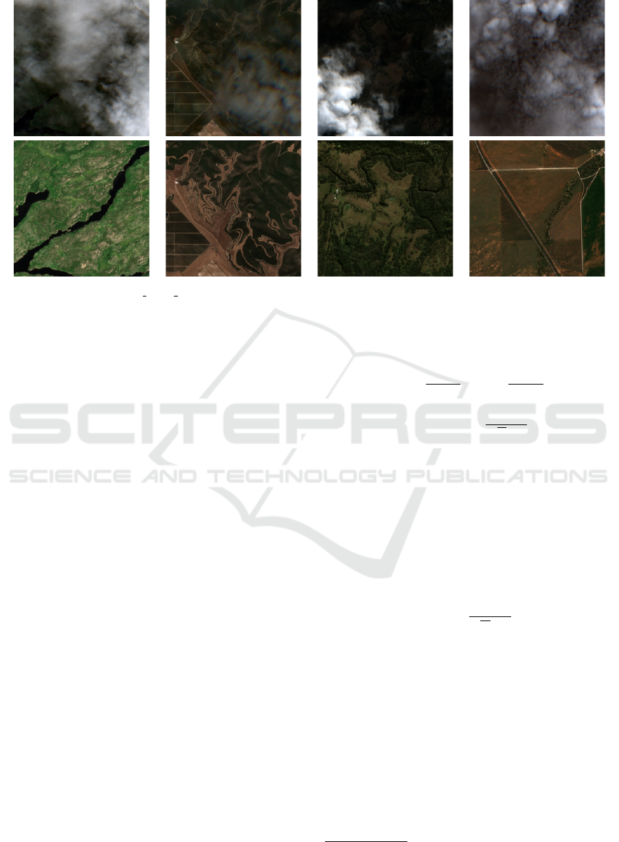
Figure 1: Samples of SEN2 MTC New dataset. The first row shows images with clouds, and the second shows the corre-
sponding cloudless images.
θ
t+1
= θ
t
−η∇
θ
J(θ
t
), (1)
where η is the learning rate, θ are the weights, and
∇
θ
J(θ
t
) is the gradient for updating the weights.
Momentum is an essential hyperparameter for
SGD, as it helps reduce large oscillations and acceler-
ates training convergence. In general terms, momen-
tum accumulates past gradients to smooth the weight
updates. This accumulation of gradients (v
t
) to mo-
mentum is defined according to Equation 2:
v
t
= γv
t−1
+ η∇
θ
J(θ
t
), (2)
where γ assigns the contribution of the previous gra-
dient (v
t−1
).
Thus, with the use of Momentum, the SGD is de-
fined according to Equation 3:
θ
t+1
= θ
t
−v
t
, (3)
Adam Kingma (2014) is an optimizer that com-
bines elements of both RMSProp and Momentum.
Specifically, it tracks an average of past gradients as
well as a mean of the squares of these gradients, en-
abling more adaptive weight updates.
Thus, the following are stored respectively: (i) ex-
ponential mean of the gradients (m
t
) and (ii) expo-
nential mean of the squares of the gradients (s
t
), as
defined by Equations 4 and 5:
m
t
= β
1
m
t−1
+ (1 −β
1
)∇
θ
J(θ
t
), (4)
s
t
= β
2
s
t−1
+ (1 −β
2
)(∇
θ
J(θ
t
))
2
, (5)
where β
1
and β
2
are the exponential decay factors.
Thus, the update of the weights in Adam occurs
according to Equations 6 and 7:
ˆm
t
=
m
t
1 −β
t
1
, ˆs
t
=
s
t
1 −β
t
2
, (6)
θ
t+1
= θ
t
−η
ˆm
t
√
ˆs
t
+ ε
, (7)
where ε is a small value to avoid zero division.
The AdamW optimizer (Loshchilov and Hutter,
2019) adapts Adam, which inserts weight decay di-
rectly into the weight update. For AdamW, the stor-
age components are the same as those in Adam: an
average of past gradients and a mean of the gradients’
squares (Equations 4 and 5). Thus, the update of the
weights of AdamW is defined according to Equation
8.
θ
t+1
= θ
t
−η

m
t
√
v
t
+ ε
+ λθ
t

, (8)
where λ is the weight decay factor.
3.4 Loss Function
Loss functions play a key role in model training by
guiding the updates of weights and gradients. In our
experiments, we used the Mean Squared Error (MSE),
Mean Absolute Error (MAE), and Huber loss func-
tions, employing their default settings in PyTorch
1
.
MAE calculates the absolute difference between
the predicted and actual values (ground truth), while
1
https://pytorch.org/docs/stable/nn.html#loss-functions
VISAPP 2025 - 20th International Conference on Computer Vision Theory and Applications
650

MSE calculates the square of this difference. These
relationships are shown in Equations 9 and 10:
MAE =
1
N
N
∑
i=1
|x
i
−y
i
|, (9)
MSE =
1
N
N
∑
i=1
(x
i
−y
i
)
2
, (10)
where x
i
is the predicted pixel value; y
i
is the the ex-
pected pixel value; and N is the number of pixels in
an image.
The Huber loss function combines aspects of
MAE and MSE, depending on a specified value of δ.
It penalizes larger errors more heavily while smooth-
ing smaller errors, as defined in Equation 11:
Huber =
(
0.5 ·(x
i
−y
i
)
2
, if |x
i
−y
i
| < δ
δ ·(|x
i
−y
i
|−0.5 ·δ), otherwise
(11)
For our experiments, as with Pytorch’s default
configuration, we used δ = 1.0.
3.5 Experimental Setup
We conducted nine experimental setups using the Dif-
fCR baseline
2
. For model training, we tested three
optimizers: AdamW, Adam, and SGD. We also eval-
uated three loss functions: Huber, MSE, and MAE. In
all experiments, we used a learning rate of 5 ×10
−5
,
a weight decay of 0.01 to mitigate overfitting, and a
batch size of 16. It is important to note that weight
decay affects each optimizer differently and directly
influences weight update dynamics. For instance,
weight decay impacts only the weights in AdamW,
whereas in SGD and Adam, it also affects the gradi-
ent. For SGD, we additionally used a momentum of
0.9.
Training was conducted for 3, 000 epochs, with
validation occurring every 200 epochs to monitor
learning progress in each experiment, using valida-
tion losses based on MAE, MSE, and Huber func-
tions. Additionally, we set a seed of 42 for all experi-
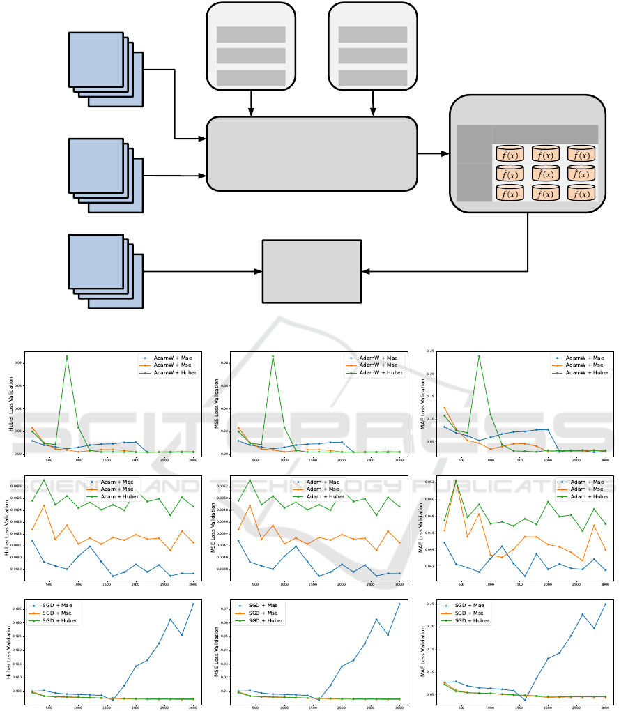
ments to ensure reproducibility. Figure 2 summarizes
the experimental design of this study.
3.6 Evaluation Metrics
The Structural Similarity Index Measure (SSIM) con-
sists of a metric used to evaluate the quality of an im-
age using a reference image. We considered a Gaus-
sian filter with a standard deviation of 1.0 for this in-
2
https://xavierjiezou.github.io/DiffCR/
dex. The SSIM metric is defined according to Equa-
tion 12
SSIM(x, y) =
(2µ
x
µ
y
+C
1
)(2σ
xy
+C
2
)
(µ
2
x
+ µ
2
y
+C
1
)(σ
2
x
+ σ
2
y
+C
2
)
, (12)
where x and y are two patches obtained from respec-
tive images to be evaluated. Values of x and y are
defined as non-negative values representing a signal,
which must be aligned; µ
x
is the pixel sample mean of
signal x; µ
y
is the pixel sample mean of signal y; σ
2
x
is
the variance of signal x; σ
2
y
is the variance of signal y;
σ
xy
is the covariance of signals x and y; C
1
and C
2
are
two constants included to avoid instability to values
very close to zero.
The Peak signal-to-noise ratio (PSNR) is another
metric for evaluating distortion between images. The
PSNR is defined in terms of MSE acording to Equa-
tion 13
PSNR = 10 log
10

255
2
MSE

(13)
3.7 Computational Environment
The experiments were performed on a PC with a 4.4
GHz Core i5-12400 CPU and 32 GB of RAM. The
PC has an NVIDIA RTX 4090 GPU (24 GB mem-
ory). The experiments used Python 3.10.14 program-
ming language and NumPy and Matplotlib libraries
for numerical processing and visualization of images
and data. The Scikit-learn library was used to manip-
ulate the set of images and analyze the classification
results. The library used to implement the deep neural
network models was PyTorch 2.3.1 and CUDA 12.1.
4 RESULTS
Validation is a crucial step in monitoring a model’s
learning process to understand its behavior, avoid
overfitting, and make targeted adjustments. In this
study, we evaluated validation loss for all experiments
using the MAE, MSE, and Huber loss functions, as
shown in Figure 3. The figure indicates that the model
overfits only in the configuration of SGD + MAE loss.
For the other configurations, a reduction in validation
loss suggests effective learning. Validation also re-
veals that the model performs better with the Adam
and AdamW optimizers across all loss functions, par-
ticularly AdamW, which exhibits less severe oscilla-
tions.
We assessed the trained models on the full
SEN2
MTC New test set using PSNR and SSIM met-
rics. Table 1 consolidates these results, showing
Evaluating Combinations of Optimizers and Loss Functions for Cloud Removal Using Diffusion Models
651

DiffCR
Optimizers:
...
Train
...
Val.
...
Test
Losses:
PSNR
SSIM
AdamW
Adam
SGD
MAE
MSE
Hubber
TRAINED MODELS
SEN2_MTC_New
MAE MSE Hubber
AdamW
Adam
SGD
Figure 2: Experimental design of this work.
(a) (b) (c)
Figure 3: Model Validation every 200 epochs. Columns (a), (b), and (c) present the validation in terms of Huber Loss
Validation, MSE Loss Validation, and MAE Loss Validation, respectively. Each row represents the AdamW, Adam, and SGD
optimizers, respectively, with each optimizer having three training loss functions.
the mean, standard deviation, and maximum value
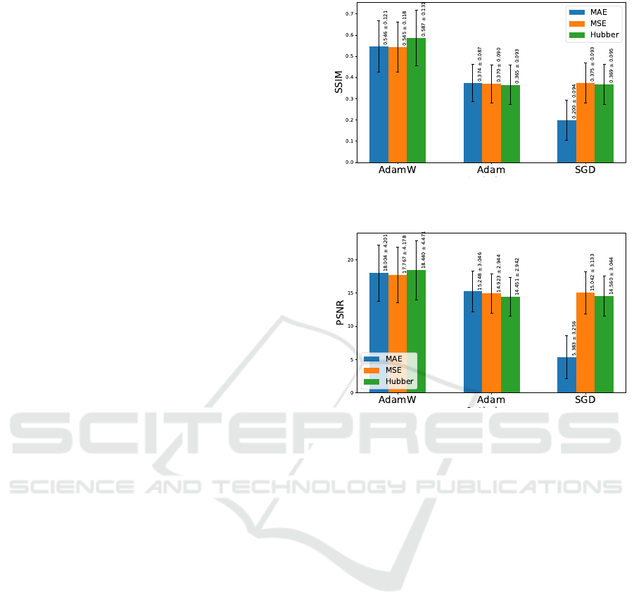
achieved by each model for both metrics. Figures 4
and 5 further illustrate these results visually.
Overall, the best results were obtained with the
AdamW optimizer. This optimizer generally provides
a stable PSNR and SSIM across the three loss func-
tions. However, while the mean values for PSNR re-
main close (around 17–18 dB) for MAE and MSE
losses, the Huber loss shows a slight increase in SSIM
(0.5871) and a significantly higher maximum PSNR
VISAPP 2025 - 20th International Conference on Computer Vision Theory and Applications
652

(32.3323). The Huber function’s selective penaliza-
tion of larger errors may have contributed to the supe-
rior performance, as it avoids uniform penalization re-
gardless of error magnitude. This configuration effec-
tively addresses cloud removal in images containing
varied contexts (e.g., rivers, forests, urban areas) and
diverse cloud types and densities, treating areas with
heavier cloud cover more stringently to produce real-
istic images. Additionaly, these results may indicate
that the Huber loss can better handle noisy or outlier
data, which could explain the significant increase in
PSNR.
In the experiments with the Adam optimizer, the
differences between loss functions are relatively mi-
nor. While there is some variation, no configuration
offers a significant performance boost. This implies
that Adam might not benefit as much from tuning
the loss function in this application, offering limited
flexibility for improvement without switching opti-
mizers. Unlike AdamW, however, the worst overall
result was recorded with Huber Loss, while the best
was achieved with MAE Loss, suggesting that Adam
might introduce more abrupt updates during training.
This optimizer generally achieves lower PSNR and
SSIM values across all loss functions when compared
to AdamW. This suggests that Adam may not be as
effective for optimizing these image quality metrics,
potentially due to the optimizer’s sensitivity to hyper-
parameter settings.
Finally, for the SGD optimizer, both MSE and Hu-
ber losses offer a more stable and moderate perfor-
mance for PSNR and SSIM, except for the overfitted
SGD + MAE model. Given the dataset’s heteroge-
neous nature, we observed substantial standard devi-
ations across all experiments, which underscores the
challenges posed by diverse land covers. SGD with
MAE loss yields the lowest average PSNR (5.3825 ±
3.2556) and a significantly lower SSIM (0.1996 ±
0.0944), indicating instability or poor convergence
in this combination. However, the maximum PSNR
achieved (17.8467) suggests that this combination can
sometimes produce reasonable outputs, although it’s
inconsistent. Further research into hyperparameter
tuning could help improve performance in such var-
ied contexts, refining the model to reduce deviations
and enhance diffusion model generalization.
For qualitative evaluation, Figures 6 and 7 present
results from two image patches (with corresponding
cloudy and cloudless references) across all experi-
ments. These figures show how the results align with
the quantitative findings. The examples represent dif-
ferent land cover types, cloud densities, and shad-
owing, highlighting challenges such as shadowed re-
gions and heavy cloud cover. Figure 6 depicts a highly
Figure 4: Visualization and comparison of SSIM metric re-
sults in the test set for each model.
Figure 5: Visualization and comparison of PSNR metric re-
sults in the test set for each model.
clouded area with minimal visible ground informa-
tion, while Figure 7 shows a less clouded region with
prominent shadows. Across all experiments, han-
dling shadowed areas remains a consistent challenge,
akin to the difficulty observed with thick clouds. The
“AdamW + Huber” combination achieves a visual re-
sult that closely matches the expected outcome, with
the most notable differences occurring in areas of
denser cloud cover. Other combinations exhibit vari-
ous reconstruction issues, including loss of informa-
tion that was originally visible and unobstructed by
clouds. Additionally, other optimizer combinations
struggle to accurately reconstruct aspects of the im-
age, such as tonality and texture, even in visible re-
gions, with “SGD + MAE” failing to generate a co-
herent image.
5 CONCLUSIONS
The selection of an optimizer and cost function
has a significant impact on training latent diffusion
models. For the cloud removal task, this study
demonstrated that these choices directly affect model
performance, either enhancing or hindering results.
Evaluating Combinations of Optimizers and Loss Functions for Cloud Removal Using Diffusion Models
653

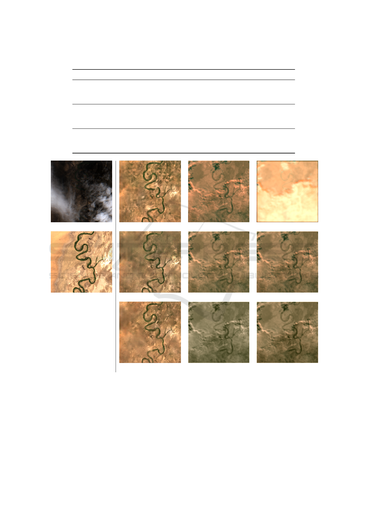
Table 1: Experimental Results for Test Set.
Optimizer Loss PSNR ↑ SSIM ↑ Max PSNR Max SSIM
AdamW
MAE 18.0040 ±4.2008 0.5463 ±0.1210 28.4146 0.8115
MSE 17.7674 ±4.1784 0.5447 ±0.1181 27.8317 0.8433
Huber 18.4395 ±4.4706 0.5871 ±0.1313 32.3323 0.8903
Adam
MAE 15.2478 ±3.0464 0.3745 ±0.0873 22.6487 0.6597
MSE 14.9229 ±2.9440 0.3704 ±0.0902 21.0076 0.6169
Huber 14.4507 ±2.9423 0.3653 ±0.0926 20.0854 0.6143
SGD
MAE 5.3825 ±3.2556 0.1996 ±0.0944 17.8467 0.6674
MSE 15.0421 ±3.1325 0.3748 ±0.0929 21.1497 0.6193
Huber 14.5604 ±3.0442 0.3688 ±0.0946 20.2948 0.6237
Cloud AdamW + MAE Adam + MAE SGD + MAE
Ground Truth AdamW + MSE Adam + MSE SGD + MSE
AdamW + Huber Adam + Huber SGD + Huber
Figure 6: Qualitative results of our experiments. The first column presents one of three multitemporal patches with clouds and
respective Ground Truth (cloudless). The other patches present visualizations of each of the nine experiments of this work.
In particular, the combination of the Huber func-
tion with the AdamW optimizer proved effective
for cloud removal, given the complex nature of
the problem, which involves varying cloud types,
ground cover, and shadows, each posing unique lo-
cal challenges for reconstruction. AdamW facilitated
smoother training, while the Huber loss function ef-
fectively emphasized regions with higher cloud occlu-
sion, preserving areas that were already cloud-free.
For future work, we plan to explore alternatives
to the TCFBlock from the DiffCR baseline, broaden
the hyperparameter search space (e.g., learning rate
and weight decay), and implement an early stopping
strategy.
VISAPP 2025 - 20th International Conference on Computer Vision Theory and Applications
654

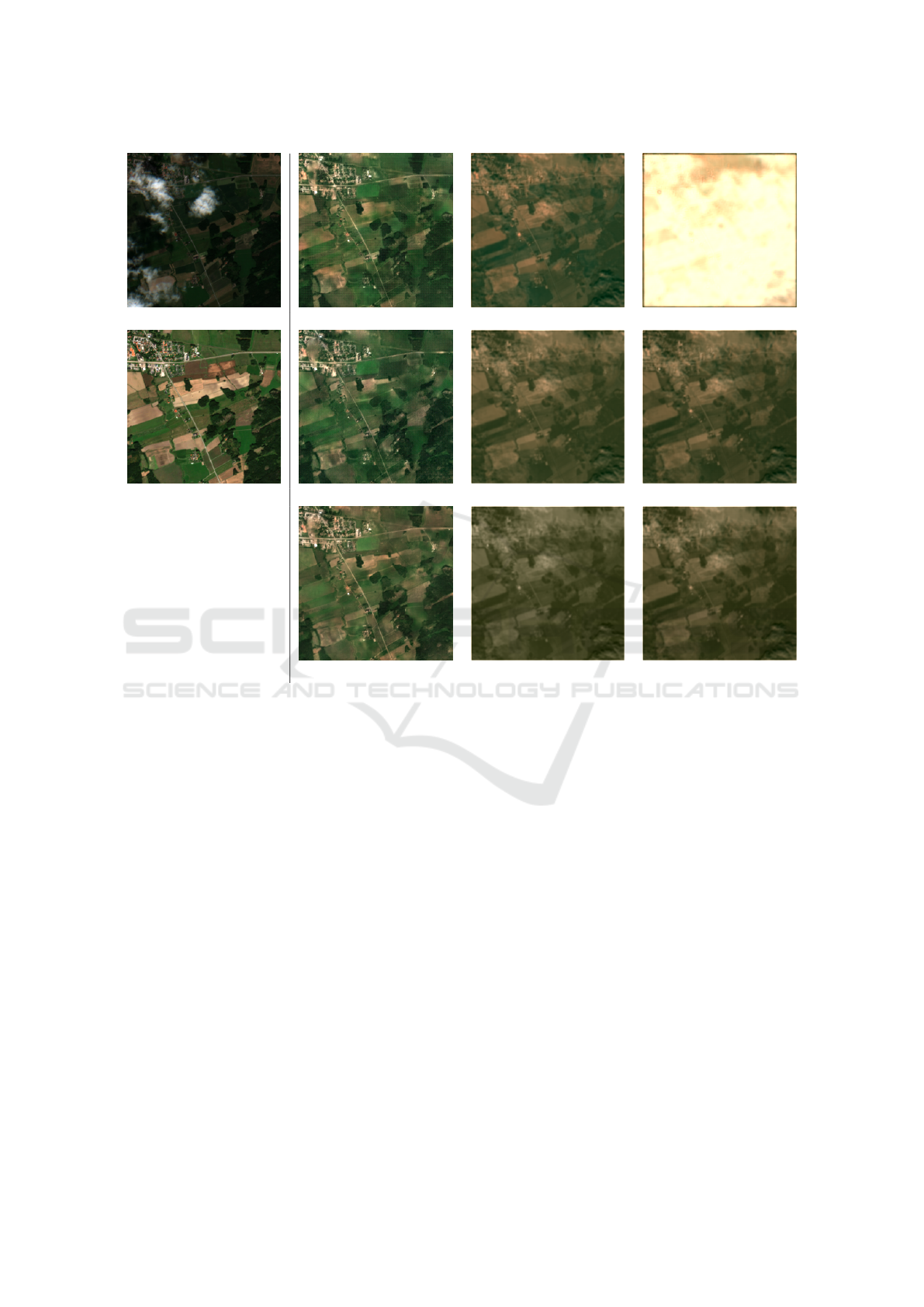
Cloud AdamW + MAE Adam + MAE SGD + MAE
Ground Truth AdamW + MSE Adam + MSE SGD + MSE
AdamW + Huber Adam + Huber SGD + Huber
Figure 7: Qualitative results of our experiments. The first column presents one of three multitemporal patches with clouds and
respective Ground Truth (cloudless). The other patches present visualizations of each of the nine experiments of this work.
ACKNOWLEDGEMENTS
We would like to thank FAPEMIG, Brazil (Grant
number CEX - APQ-02964-17) for financial support.
Andr
´
e R. Backes gratefully acknowledges the finan-
cial support of CNPq (National Council for Scien-
tific and Technological Development, Brazil) (Grant
#307100/2021-9). This study was financed in part by
the Coordenac¸
˜
ao de Aperfeic¸oamento de Pessoal de
N
´
ıvel Superior - Brazil (CAPES) - Finance Code 001.
REFERENCES
Arakaki, L. G., Silva, L. H. F. P., da Silva, M. V., Melo,
B. M., Backes, A. R., Escarpinati, M. C., and Mari,
J. F. (2023). Evaluation of u-net backbones for cloud
segmentation in satellite images. In Proceedings of
the 18th International Joint Conference on Computer
Vision, Imaging and Computer Graphics Theory and
Applications (VISIGRAPP 2023) - Volume 4: VIS-
APP, pages 452–458. INSTICC, SciTePress.
Barbosa, G., Moreira, L., de Sousa, P. M., Moreira, R., and
Backes, A. (2024). Optimization and learning rate in-
fluence on breast cancer image classification. In Pro-
ceedings of the 19th International Joint Conference
on Computer Vision, Imaging and Computer Graphics
Theory and Applications - Volume 3: VISAPP, pages
792–799. INSTICC, SciTePress.
Dong, S., Wang, P., and Abbas, K. (2021). A survey on
deep learning and its applications. Computer Science
Review, 40:100379.
Ebel, P., Garnot, V. S. F., Schmitt, M., Wegner, J. D., and
Zhu, X. X. (2023). Uncrtaints: Uncertainty quantifi-
cation for cloud removal in optical satellite time se-
ries. In Proceedings of the IEEE/CVF Conference
on Computer Vision and Pattern Recognition, pages
2085–2095.
Ferreira, J. R., Silva, L. H. F. P., Escarpinati, M. C., Backes,
A. R., and Mari, J. F. (2024). Evaluating multi-
ple combinations of models and encoders to segment
clouds in satellite images. In Proceedings of the 19th
Evaluating Combinations of Optimizers and Loss Functions for Cloud Removal Using Diffusion Models
655

International Joint Conference on Computer Vision,
Imaging and Computer Graphics Theory and Applica-
tions - Volume 3: VISAPP, pages 233–241. INSTICC,
SciTePress.
Huang, G.-L. and Wu, P.-Y. (2022). Ctgan: Cloud
transformer generative adversarial network. In 2022
IEEE International Conference on Image Processing
(ICIP), pages 511–515. IEEE.
Jeppesen, J. H., Jacobsen, R. H., Inceoglu, F., and Tofte-
gaard, T. S. (2019). A cloud detection algorithm for
satellite imagery based on deep learning. Remote
sensing of environment, 229:247–259.
Kingma, D. P. (2014). Adam: A method for stochastic op-
timization. arXiv preprint arXiv:1412.6980.
Loshchilov, I. and Hutter, F. (2019). Decoupled weight de-
cay regularization.
Podsiadlo, I., Paris, C., and Bruzzone, L. (2020). A study
of the robustness of the long short-term memory clas-
sifier to cloudy time series of multispectral images.
In Image and Signal Processing for Remote Sensing
XXVI, volume 11533, pages 335–343. SPIE.
Robbins, H. and Monro, S. (1951). A stochastic approxi-
mation method. The annals of mathematical statistics,
pages 400–407.
Ronneberger, O., Fischer, P., and Brox, T. (2015). U-net:
Convolutional networks for biomedical image seg-
mentation.
Ruder, S. (2017). An overview of gradient descent opti-
mization algorithms.
Seyrek, E. C. and Uysal, M. (2024). A comparative anal-
ysis of various activation functions and optimizers in
a convolutional neural network for hyperspectral im-
age classification. Multimedia Tools and Applications,
83(18):53785–53816.
Wang, Z., Zhou, D., Li, X., Zhu, L., Gong, H., and
Ke, Y. (2023). Virtual image-based cloud removal
for landsat images. GIScience & Remote Sensing,
60(1):2160411.
Xie, Y., Li, Z., Bao, H., Jia, X., Xu, D., Zhou, X., and
Skakun, S. (2023). Auto-cm: Unsupervised deep
learning for satellite imagery composition and cloud
masking using spatio-temporal dynamics. In Proceed-
ings of the AAAI Conference on Artificial Intelligence,
volume 37, pages 14575–14583.
Zhao, M., Olsen, P., and Chandra, R. (2023). Seeing
through clouds in satellite images. IEEE Transactions
on Geoscience and Remote Sensing, 61:1–16.
Zhao, X. and Jia, K. (2023). Cloud removal in remote sens-
ing using sequential-based diffusion models. Remote
Sensing, 15(11):2861.
Zou, X., Li, K., Xing, J., Zhang, Y., Wang, S., Jin, L., and
Tao, P. (2024). Diffcr: A fast conditional diffusion
framework for cloud removal from optical satellite im-
ages. IEEE Transactions on Geoscience and Remote
Sensing, 62:1–14.
VISAPP 2025 - 20th International Conference on Computer Vision Theory and Applications
656