Investigating the Propagation of CT Acquisition Artifacts

along the Medical Imaging Pipeline

Jakob Peischl and Renata G. Raidou

Institute of Visual Computing & Human-Centered Technology, TU Wien, Favoritenstrasse 9-11, 1060, Vienna, Austria

Keywords:

Uncertainty Quantiﬁcation and Propagation, Medical Imaging, Medical Image Analysis and Visualization.

Abstract:

We propose a framework to support the simulation, exploration, and analysis of uncertainty propagation in

the medical imaging pipeline—exempliﬁed with artifacts arising during CT acquisition. Uncertainty in the

acquired data can affect multiple subsequent stages of the medical imaging pipeline, as artifacts propagate and

accumulate along the latter, inﬂuencing the diagnostic power of CT and potentially introducing biases in even-

tual decision-making processes. We designed and developed an interactive visual analytics framework that

simulates real-world CT artifacts using mathematical models, and empowers users to manipulate parameters

and observe their effects on segmentation outcomes. By extracting radiomics features from artifact-affected

segmented images and analyzing them using dimensionality reduction, we uncover distinct patterns related to

individual artifacts or combinations thereof. We demonstrate our proposed framework on use cases simulat-

ing the effects of individual and combined artifacts on segmentation outcomes. Our application supports the

effective and ﬂexible exploration and analysis of the impact of uncertainties on the outcomes of the medical

imaging pipeline. Initial insights into the nature and patterns of the simulated artifacts could also be derived.

1 INTRODUCTION

Medical imaging is foundational to modern medicine,

aiding in disease prevention, diagnosis, and treatment.

Imaging modalities like Computed Tomography (CT)

and Magnetic Resonance Imaging (MRI) provide

patient-speciﬁc information based on physical prin-

ciples that capture dedicated tissue characteristics to

support clinical decisions (Gillmann et al., 2021).

However, data uncertainties stemming from several

factors, such as low spatial resolution, artifacts, or

hardware/software issues, are often present (Ristovski

et al., 2014; Gillmann et al., 2021). This causes dis-

crepancies between the physical properties of imaged

tissue and the respective image representation. These

uncertainties are subsequently propagated through

the medical imaging pipeline, affecting all the remain-

ing steps of processing, segmentation, mapping, and

rendering (Preim and Botha, 2013)—potentially, im-

pacting the accuracy of diagnosis and treatment.

Uncertainty in medical imaging can affect mul-

tiple stages of the medical imaging pipeline, with

signiﬁcant challenges at each step (Schlachter et al.,

2019). For example, in CT data acquisition we often

encounter artifacts due to patient motion and partial

https://orcid.org/0000-0003-2468-0664

volume artifacts. Such artifacts may further propa-

gate and accumulate during pre-processing, segmen-

tation, and mapping, inﬂuencing the diagnostic power

of the employed data and potentially introducing bi-

ases in eventual decision-making processes (Raidou,

2018). For decisions involving artiﬁcial intelligence

(AI), uncertainty can additionally compromise model

reliability (Zhou et al., 2021). Whether the “decision

maker” is an AI model or a human, recognizing and

mitigating uncertainties is essential.

This paper focuses on understanding the propaga-

tion of acquisition uncertainty, exempliﬁed with CT

imaging. CT is integral to numerous clinical pro-

cesses, for which the presence of potential uncertain-

ties is often critical. Motion artifacts, partial vol-

ume effects, and ring artifacts are among the most

prevalent uncertainties that impact CT imaging qual-

ity (Preim and Botha, 2013). By examining these ar-

tifacts, we aim to map the ways uncertainties in the

acquisition step of the medical imaging pipeline af-

fect subsequent steps—and in particular, the last step

of analysis.

To this end, we introduce a methodology to simu-

late and investigate the propagation of CT acquisition

uncertainty using mathematical models that describe

the aforementioned, common artifacts. Our proposed

752

Peischl, J. and Raidou, R. G.

Investigating the Propagation of CT Acquisition Artifacts along the Medical Imaging Pipeline.

DOI: 10.5220/0013254200003912

Paper published under CC license (CC BY-NC-ND 4.0)

In Proceedings of the 20th International Joint Conference on Computer Vision, Imaging and Computer Graphics Theory and Applications (VISIGRAPP 2025) - Volume 1: GRAPP, HUCAPP

and IVAPP, pages 752-764

ISBN: 978-989-758-728-3; ISSN: 2184-4321

methodology involves a user-in-the-loop approach for

constructing uncertainty pipelines by combining ar-

tifacts to model their effects on the acquired im-

ages, and their impact on the subsequent segmenta-

tion. Making use of radiomics feature extraction and

unsupervised learning approaches, we visualize and

analyze segmentation outcomes from artifact-affected

images. In this way, we can evaluate in real time

how acquisition uncertainty has propagated through

the pipeline and the magnitude of its impact on di-

agnostic information. Although our focus is on CT

artifacts, the proposed methodology can be adapted

to other modalities, allowing for broader applicability

in medical imaging uncertainty research.

Our contributions to the ﬁeld of uncertainty visu-

alization include the introduction of a novel frame-

work for acquisition uncertainty analysis in medical

imaging, an interactive application for the investiga-

tion of simulated uncertainty pipelines, and a demon-

stration of use cases that illustrate the potential of our

approach in a real-life setting.

2 RELATED WORK

In this section, we provide an overview of different

uncertainty types and examine relevant literature on

uncertainty quantiﬁcation and propagation, with a fo-

cus on medical imaging.

Uncertainty types are classiﬁed as either epis-

temic or aleatoric (Potter et al., 2012). Epistemic

uncertainty results from model imperfections and can

be reduced by improved measurements or calibration,

while aleatoric uncertainty arises from inherent ran-

domness and is typically represented with probabil-

ity density functions (PDFs). Given that CT image

artifacts are often reducible or avoidable, our work

focuses on epistemic uncertainty. However, our em-

ployed methods could theoretically extend to aleatoric

uncertainties.

We target speciﬁc medical imaging pipeline

steps that we anticipate to be affected by uncer-

tainties (Gillmann et al., 2021). Each step intro-

duces new uncertainties: acquisition uncertainties

may arise from physical model assumptions, segmen-

tation algorithms add model-based and parameter un-

certainties affecting boundary delineations, and map-

ping, e.g., via marching cubes (Lorensen and Cline,

1987), introduces approximations to the derived sur-

face meshes. In this study, segmentation and mapping

are kept invariant to investigate in an isolated manner

uncertainties only from the acquisition step.

(Ristovski et al., 2014) and (Gillmann et al., 2021)

recently authored surveys for uncertainty classiﬁca-

tion in medical applications. Ristovski et al. clas-

sify uncertainties using random ﬁelds to represent ar-

bitrary probability distribution functions. By deter-

mining the mathematical characteristics of a random

ﬁeld, they provide a framework to consider uncer-

tainty propagation behavior. Gillmann et al. review

state-of-the-art uncertainty-aware visualization tech-

niques related to medical imaging applications, ex-

plore pipeline combinations, and identify challenges

in creating comprehensive uncertainty-aware medical

imaging workﬂows.

Uncertainty quantiﬁcation and propagation re-

quires formalized mathematical models to track how

uncertainties propagate within an imaging pipeline. A

general formulation utilizes PDFs, where each input

of the input vector X = (X

, . . . , X

)

is given as a

PDF f

). The challenge is then to ﬁnd the PDF of

the output Y after it has been transformed by the func-

tion g, i.e., ﬁnding f

(y) where Y = g(X). Various ap-

proaches for determining the output uncertainty in the

so-called forward uncertainty quantiﬁcation problem

exist (Brodlie et al., 2012). For complex uncertain-

ties, Monte-Carlo-based techniques that approximate

(y) are often necessary (Brodlie et al., 2012). A

primary drawback of these methods is computational

inefﬁciency due to slow convergence. Analytical so-

lutions would be more efﬁcient but are unavailable for

arbitrary PDF propagation.

Uncertainty quantiﬁcation has become a relevant

aspect of a wide range of scientiﬁc ﬁelds (Zhang,

2021). Uncertainty-handling frameworks have

been proposed for instance by (Roy and Oberkampf,

2011) to model, estimate, and propagate through any

scientiﬁc model uncertainties. (Wu et al., 2012) focus

on explorative aspects of uncertainty and build an in-

teractive tool that visualizes uncertainty ﬂows along a

data processing pipeline—under the assumption that

input uncertainties follow a multivariate normal dis-

tribution. Again, the output uncertainty is estimated

using Monte Carlo sampling.

The application of uncertainty quantiﬁcation

within medical imaging has primarily focused on vi-

sualization and single-stage analysis of uncertainty

within images. For example, (Howard et al., 2014)

use sampling-based CT uncertainty quantiﬁcation,

and (Gillmann et al., 2017) employ analytical meth-

ods to highlight image noise as a primary uncertainty

source. (Tian and Samei, 2016) model CT quantum

noise, and (Gravel et al., 2004) examine noise pro-

ﬁles across modalities. (Diwakar and Kumar, 2018)

consolidate insights into CT noise, highlighting de-

noising as a key challenge.

There is limited literature on uncertainty prop-

agation across multiple stages of medical imaging

Investigating the Propagation of CT Acquisition Artifacts along the Medical Imaging Pipeline

753

Acquisition

Artifacts

. . .

Pipeline Groups

. . .

Segmentation

. . .

Feature

Extraction















, . ..





















, . ..





















, . ..







Data

Analysis

PCA

and

t-SNE

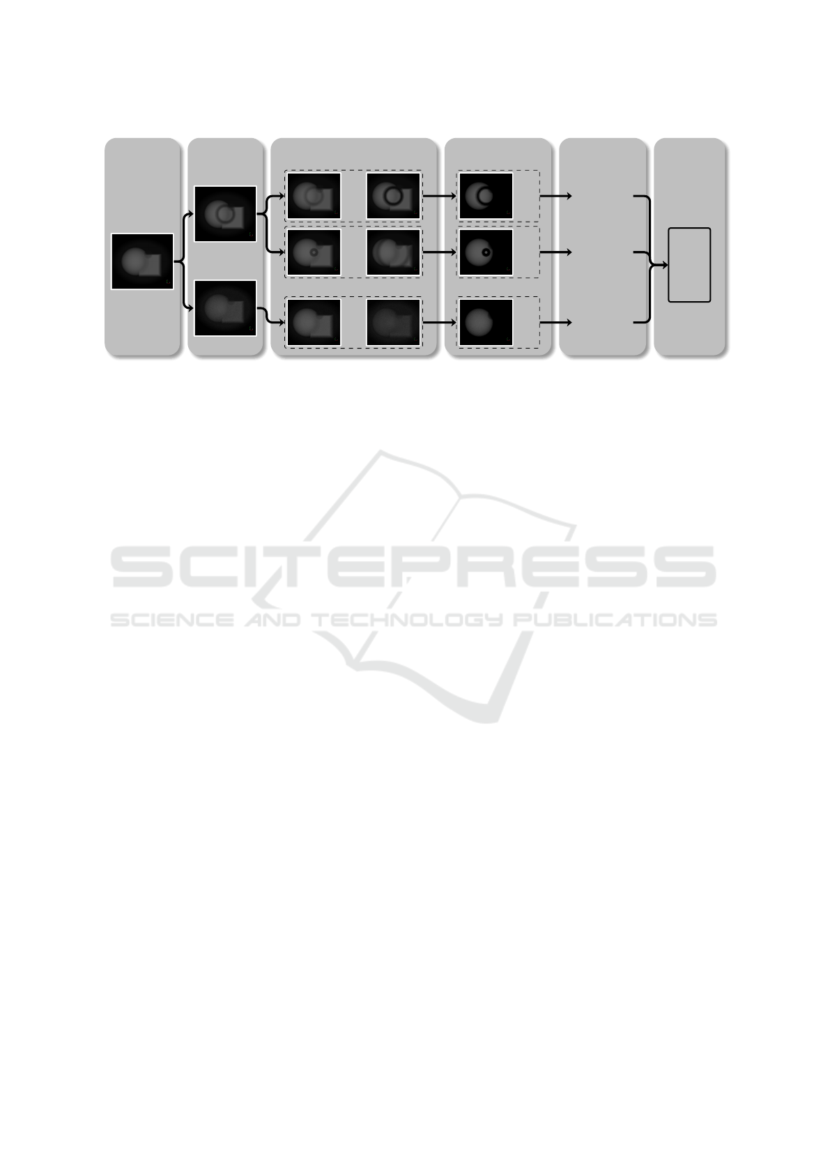
Figure 1: Overview of the workﬂow adopted in our approach. The workﬂow comprises ﬁve steps: acquisition, artifact gen-

eration, pipeline grouping, segmentation, and outcome analysis (which consists of two substeps: radiomics feature extraction

and analysis based on dimensionality reduction).

pipelines. A notable exception is Diffusion Ten-

sor Imaging (DTI), where (Behrens et al., 2003)

laid the groundwork for uncertainty propagation from

diffusion-weighted signals to tensor-derived quanti-

ties. Yet, DTI ﬁndings are not generalizable to CT

due to modality-speciﬁc differences in imaging re-

construction and clinical use cases. Recent advance-

ments in deep learning (DL) have created interest in

both epistemic and aleatoric uncertainty quantiﬁca-

tion and propagation within medical imaging (Feiner

et al., 2023). However, CT artifacts affecting DL

models in real-world scenarios remain underexplored.

Only (Athanasiou et al., 2015) explored multi-stage

error propagation within imaging pipelines for plaque

classiﬁcation, linking acquisition and segmentation

errors to classiﬁcation accuracy. In contrast, our work

evaluates outcomes based on radiomics feature com-

parisons to obtain a holistic view of CT uncertainties

across pipeline stages.

3 METHODOLOGY

In this chapter, we present our proposed methodol-

ogy for the interactive quantiﬁcation and propaga-

tion of CT uncertainties through the medical imaging

pipeline. The workﬂow involves ﬁve stages, which

are depicted in Fig. 1 and further described in the up-

coming subsections. We ﬁrst generate an uncertainty-

free base image during the image acquisition stage

(Sec. 3.1). Users can then add artifacts, whose effects

are applied to this base image in the artifacts genera-

tion stage (Sec. 3.2). The pipeline grouping stage al-

lows users to combine different artifacts and specify

valid parameters for each of them (Sec. 3.3). We then

proceed with the segmentation step to calculate seg-

mentations of the artifact-affected images (Sec. 3.4).

Next, we extract radiomics features from the outcome

segmentations and comparatively analyze them using

a combination of principal component analysis (PCA)

and t-distributed stochastic neighbor embedding (t-

SNE), inspired by the previous work of (Reiter et al.,

2018) (Sec. 3.5). This is the outcome analysis stage.

Our interface facilitates these steps, targeting medical

imaging researchers and CT imaging professionals in-

terested in uncertainty quantiﬁcation and propagation.

3.1 Image Acquisition

At the image acquisition stage, we deﬁne the extent,

i.e. the physical dimensions, and spatial resolution

of the CT input volume. A CT dataset can be de-

ﬁned mathematically as a function I : R

→ R that

maps a three-dimensional spatial position (x, y, z) to

a corresponding voxel value I(x, y, z). CT voxel val-

ues (i.e. radiodensity values) are given in Hounsﬁeld

Units (HU), proportional to the attenuation coefﬁcient

normalized to water (Yucel-Finn et al., 2023). Users

can deﬁne voxel values through implicit modeling or

direct image import. In the former case, users employ

constructive solid geometry to model complex objects

from primitive shapes (Laidlaw et al., 1986). This ap-

proach provides structural information for subsequent

stages and it is showcased in Fig. 2 (a). In the lat-

ter case, users can import image data allowing for a

more realistic data analysis (Fig. 2 (b)). When choos-

ing this option, artifact simulation might be limited,

and the image may already suffer from some kind of

uncertainty. For simplicity, our workﬂow assumes an

idealized, artifact-free CT acquisition.

IVAPP 2025 - 16th International Conference on Information Visualization Theory and Applications

754

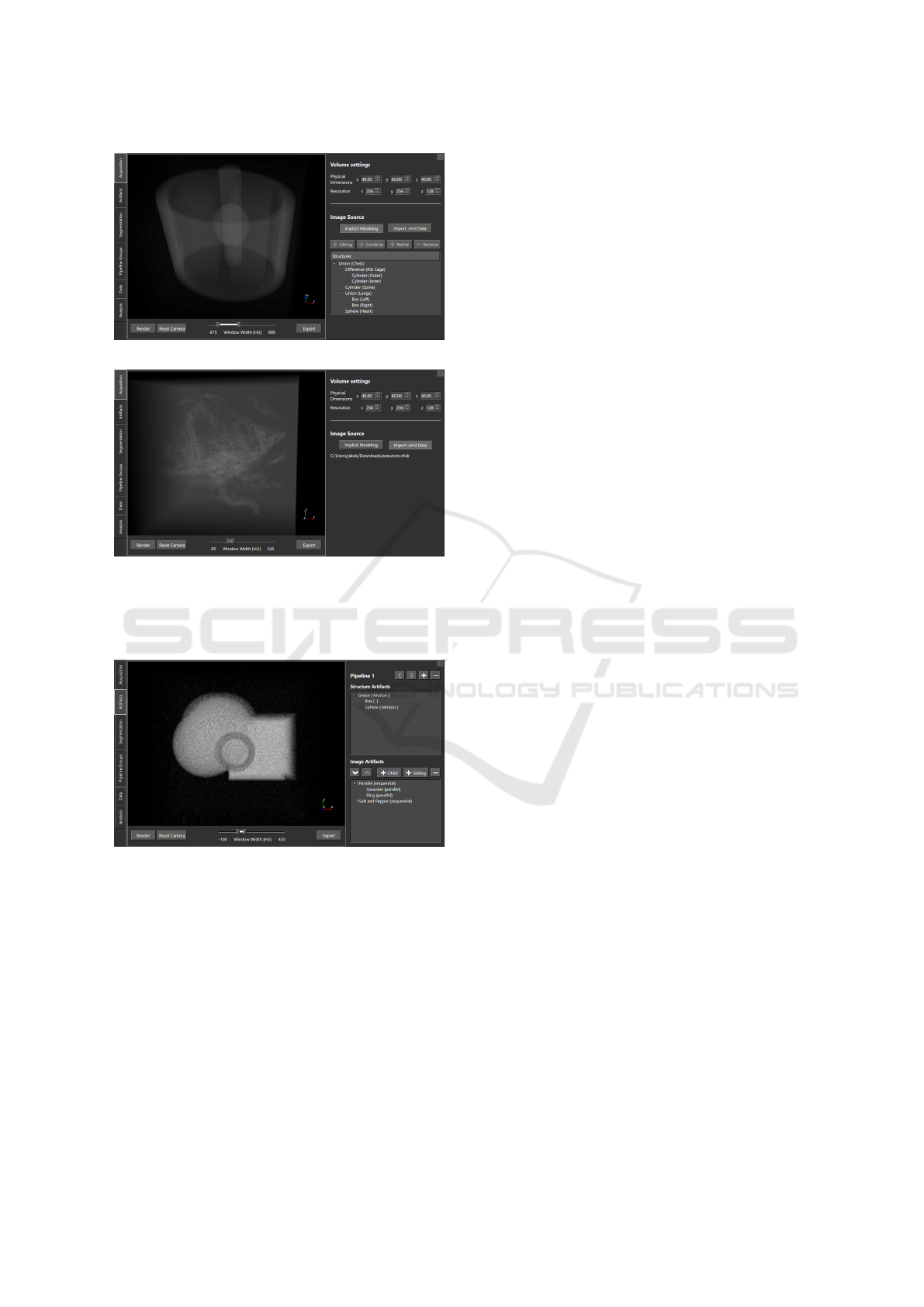
(a)

(b)

Figure 2: In the image acquisition stage, the user can

generate data by (a) implicit modeling or by (b) direct

image import (here, a CT angiogram containing a brain

aneurysm (Klacansky, 2017)).

Figure 3: In the artifacts generation stage, the user deﬁnes

which artifacts are to be simulated and in which order. Here,

two artifacts are simulated and combined: a motion artifact

(comprising a Gaussian blur and a ring artifact), and salt

and pepper noise. The order in which artifacts are applied

is speciﬁed in the bottom-right corner of the interface.

3.2 Artifacts Generation

In this stage, users deﬁne which artifacts they would

like to simulate on the data obtained from the ﬁrst step

(Fig. 3). Rather than simulating CT acquisition, we

assume an artifact-free CT image, to which artifact

effects are added. This ensures a ﬂexible simulation

across scanning technologies by adjusting artifact pa-

rameters. Multiple artifact sets can also be created

and are combined later, in the stage where pipeline

groups are simulated (Sec. 3.3).

Our framework separates potential CT artifacts

into two types: image artifacts and structure artifacts

(Fig. 4). Image artifacts apply to the entire CT volume

based on voxel-speciﬁc radiodensity without needing

structural information. For example, a Gaussian noise

artifact adds random noise to each voxel, as deter-

mined by a user-deﬁned Gaussian distribution. Con-

versely, structure artifacts affect speciﬁc structures (or

subregions within an image); thus, they need addi-

tional positional information. For instance, a motion

artifact would affect a structure by shifting it and by

applying a Gaussian blur, as shown in Fig. 3. Simulat-

ing this is only possible if the positional information

of the affected structure is known. Both types of arti-

facts are further discussed below.

Artifacts can be applied sequentially or in parallel

on a given dataset. For image artifacts, we can apply

artifacts sequentially, in parallel, or in a (potentially

nested) combination of both approaches, as shown in

the bottom-right corner of the interface in Fig. 3. In

contrast, the effects of structure artifacts are applied

only in parallel because they are inherently localized

to speciﬁc structures within the CT image. Apply-

ing them sequentially would not make sense because

each structure artifact alters independently its associ-

ated structure without inﬂuencing others.

3.2.1 Image Artifacts

The image artifacts modeled within our approach, to-

gether with their parameters, are summarized in Fig. 4

(a)–(d). Each of these artifacts follows mathematical

descriptions, as formalized in literature and included

in our Appendix. Salt and pepper noise appears

as isolated bright (“salt”) or dark (“pepper”) voxels,

caused by rare electronic errors and is generally mi-

nor in CT imaging (Lu et al., 2018) (Fig. 4 (a)). De-

spite its limited impact, we include it here for comple-

tion. Parameters of our modeling include radioden-

sity and the relative amount of salt and pepper pixels.

Gaussian noise, observed in low-dose CT images, re-

sults from low photon counts and other electronics-

based noise (Boas and Fleischmann, 2012) (Fig. 4

(b)). Though often modeled by a Poisson distribu-

tion, a Gaussian distribution sufﬁces at high photon

counts (Madhura and Babu, 2017). The parameters

of our modeling are the mean and standard deviation

of the distribution. Cupping artifacts, due to beam

hardening, appear as shading towards the center of a

dense object (e.g. a hard bone structure) (Barrett and

Keat, 2004) (Fig. 4 (c)). The shading appears pro-

nounced in images with larger, isotropic objects like

the skull. Its modeling relies on user-deﬁned param-

Investigating the Propagation of CT Acquisition Artifacts along the Medical Imaging Pipeline

755

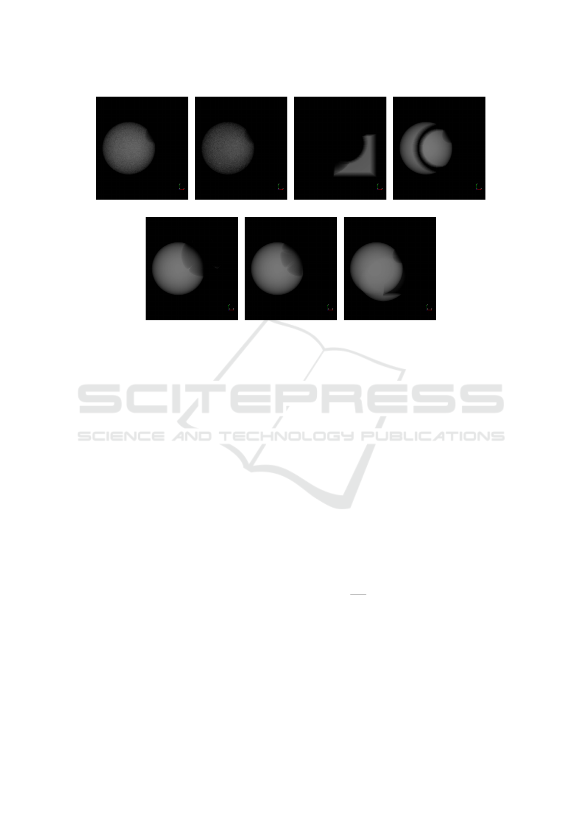
(a) Salt and pepper noise (b) Gaussian noise (c) Cupping artifact (d) Ring artifact

(e) Metal artifact (f) Windmill artifact (g) Motion artifact

Figure 4: The artifacts that can be generated as part of our approach, exempliﬁed on a simple implicitly modeled data set.

Subﬁgures (a)–(d) represent image artifacts, while (e)–(g) represent structure artifacts.

eters for center location and shading intensity. Fi-

nally, ring artifacts are caused by detector miscali-

brations, forming rings around the scanning axis, and

are sometimes mistaken for pathologies (Boas and

Fleischmann, 2012) (Fig. 4 (d)). Modeling parame-

ters include the inner radius, width, radiodensity, and

ring center location.

3.2.2 Structure Artifacts

The structure artifacts modeled within our approach,

together with their parameters, are summarized in

Fig. 4 (e)–(g). Each of these artifacts follows math-

ematical descriptions, as formalized in literature and

included in our Appendix. Metal artifacts are com-

mon in CT due to metal objects that cannot be re-

moved during acquisition (Boas and Fleischmann,

2012) (Fig. 4 (e)). These artifacts stem from effects

such as beam hardening, which causes directional

shading and photon scatter, making shading more

prominent. This artifact is modeled with assump-

tions on attenuation and distance effects, using pa-

rameters for attenuation direction and shading length.

Windmill artifacts appear as evenly spaced, bright

streaks around high-attenuation objects (Barrett and

Keat, 2004) (Fig. 4 (f)). They occur only in helical

CT and increase in number with greater pitch. The

model assumes shading decreases with distance, us-

ing parameters for radiodensity, length, and rotation

per slice. Finally, motion artifacts are frequent, of-

ten due to involuntary or internal movement of the pa-

tient, showing as blurring or double edges (Boas and

Fleischmann, 2012) (Fig. 4 (g)). The model captures

these by transforming structure locations and apply-

ing Gaussian blur to regions of motion, using param-

eters for transformation matrix and blur properties.

3.3 Pipeline Grouping

At this stage, ﬁnal artifact parameters are set for

customizable pipeline groups. Each group contains

combinations of artifact pipelines (serial, in parallel,

or (nested) combinations thereof) based on a base

pipeline, which users adjust with parameter ranges.

The primary purpose of the parameter ranges is to de-

termine a set of valid values for an artifact parameter.

For example, this enables a user to vary the standard

deviation of a Gaussian artifact contained in the base

pipeline in an interval [a, b] and a step size s, result-

ing in n = ⌊

b − a

⌋ distinct artifact pipelines, as shown

in Fig. 1. Since multiple parameter ranges may be

deﬁned per pipeline group and artifact, the total num-

ber of valid conﬁgurations for a pipeline group cor-

responds to the number of elements in the Cartesian

product of the parameter spans.

IVAPP 2025 - 16th International Conference on Information Visualization Theory and Applications

756

3.4 Segmentation

During the segmentation stage, the user can segment

a structure of interest. As we are particularly inter-

ested in the propagation of acquisition uncertainties

through the pipeline and their effect on the outcomes,

we choose to keep the segmentation ﬁlter simple and

its parameters unchanged. Therefore, we employ a

simple thresholding approach where the user only

needs to select an appropriate threshold for the seg-

mentation. An example of the segmentation outcome

of different pipeline groupings is shown in Fig. 1.

This ensures that we can later compare the resulting

feature values meaningfully since all images have un-

dergone the same segmentation—without having to

additionally consider the effects of the segmentation

step itself on the uncertainty outcomes.

3.5 Outcome Analysis

A quantitative comparison of the artifact effects on

the outcome of the pipeline is not feasible using

segmented images alone. To this end, we adopt a

radiomics-based approach, extracting predeﬁned ra-

diomics features from the segmented outcome of each

artifact-impacted pipeline. Radiomics are quantita-

tive metrics derived from medical images and are of-

ten used to characterize tumors (Gillies et al., 2016).

They consist of a series of features that describe the

morphology, texture, and intensity of a segmenta-

tion. We extract 13 3D shape features and 19 ﬁrst-

order features, chosen for their time complexity of

O(n log n) and their simpler physical interpretations.

Subsequently, to comparatively explore and ana-

lyze relationships between artifact pipelines, we em-

ploy a t-distributed stochastic neighborhood embed-

ding (t-SNE) (van der Maaten and Hinton, 2008)

and principal component analysis (PCA) (Abdi and

Williams, 2010), similar to the prior work of (Re-

iter et al., 2018). Using a Barnes-Hut algorithm for

t-SNE (van der Maaten, 2014) allows for a reduced

time complexity of O(n logn). We standardize the

feature data for equal weighting and apply t-SNE to

the entire dataset across pipeline groups (e.g. mul-

tiple artifacts with multiple parameterizations) while

using PCA within pipeline groups (e.g. one type of

artifact with several parameterizations), as shown in

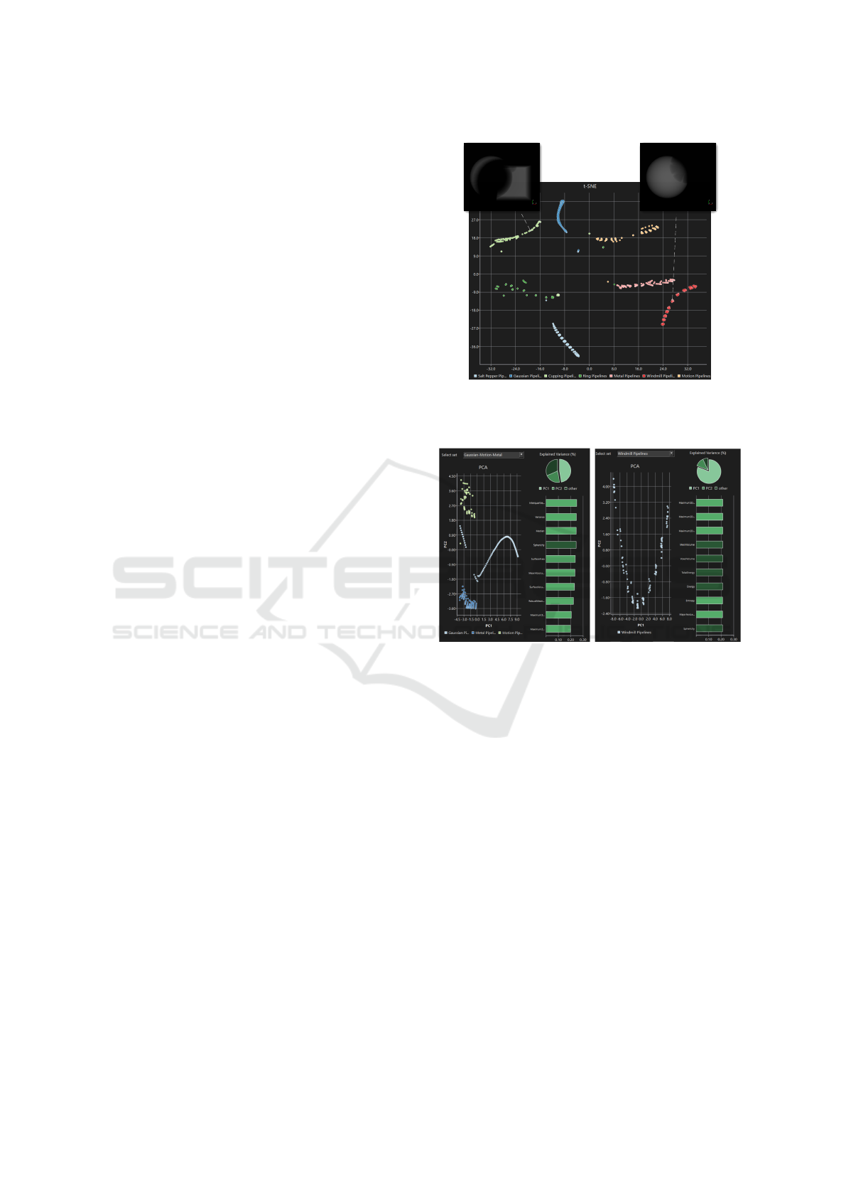
Fig. 5. The t-SNE results are represented in an in-

teractive 2D scatterplot, with data points color-coded

by pipeline group (Fig. 5 (a)). Selecting a subset of

points in the t-SNE plot triggers a PCA analysis on

this ﬁltered selection. The PCA output is also shown

in a 2D scatterplot, with insights into the PCs and their

signiﬁcance using a pie and bar chart (Fig. 5 (b)). This

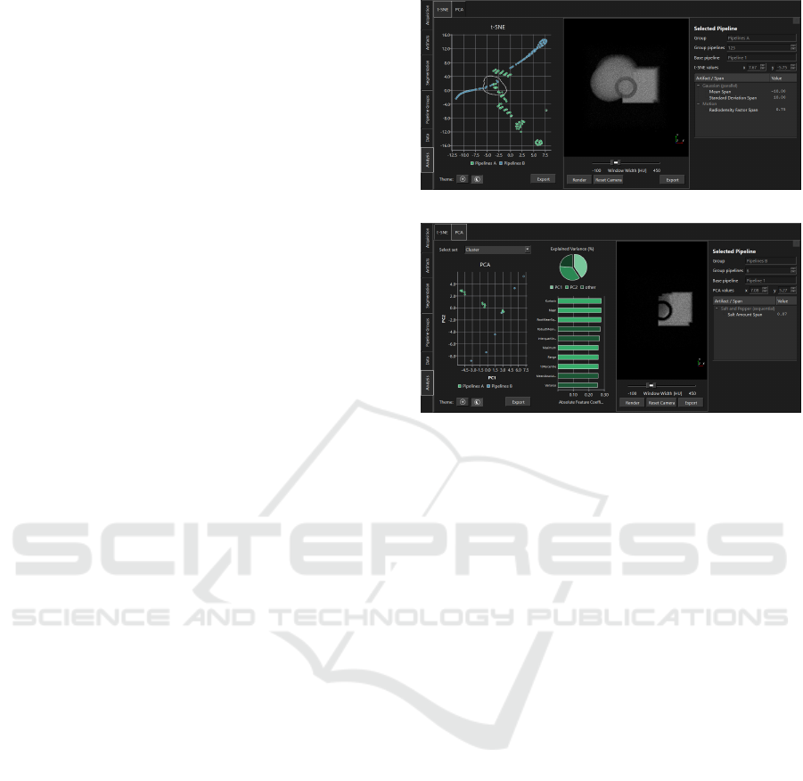
(a)

(b)

Figure 5: In the outcome analysis step, (a) we use a t-SNE

analysis to compare pipeline groups. The left window dis-

plays a scatterplot of t-SNE results for radiomic features

from each artifact-impacted pipeline. Selecting a data point

in this plot reveals the associated pipeline in the right win-

dow and renders the affected data in the center window.

Here, a cluster of points is selected on the t-SNE view us-

ing a lasso brush. (b) Next, we perform PCA analysis on

the lasso-selected points in (a). The left window shows a

scatterplot of the ﬁrst two PCs. The center and right win-

dows present a pie chart of explained variances for these

PCs with a bar chart of sorted feature coefﬁcients for PC1,

and renderings and pipeline details for the selected data.

Dark green indicates negative feature coefﬁcients.

combination leverages the ability of t-SNE to detect

non-linear relationships across pipelines and the in-

terpretability of PCA within pipelines.

3.6 Implementation

For the implementation of the framework, C++20 was

chosen for its performance capabilities and low-level

control, while the Qt framework is used for devel-

oping a cross-platform graphical user interface. For

medical image processing, the application employs

the Visualization Toolkit (VTK). Data storage utilizes

the HDF5 format with zlib compression to manage

the large memory requirements effectively. For fea-

ture extraction, PyRadiomics is used. The imple-

mentation of our approach is available on our Open-

Source Repository.

Investigating the Propagation of CT Acquisition Artifacts along the Medical Imaging Pipeline

757

4 RESULTS

This section presents the results of our uncertainty

propagation framework applied to two scenarios. We

describe each scenario and analyze the results, fol-

lowed by a cumulative summary and discussion. The

selected scenarios are intended to demonstrate the ca-

pabilities of our proposed solution with examples rep-

resenting both implicitly modeled and imported data.

Each scenario was designed to enable insights rele-

vant to real-world cases, using CT data and artifact

parameters that reﬂect realistic parameter ranges.

4.1 Scenario 1: Modeled Data

The ﬁrst example scenario uses implicitly modeled CT

data. We created a CT structure scene that is chal-

lenging for segmentation by placing structures with

similar radiodensities close to a structure of inter-

est. We added both image and structure artifacts (see

Fig. 4), making segmentation more complex and anal-

ysis more meaningful for a real-life scenario. This

setup aims to simulate applications like cardiac and

pelvic organ CT segmentation, where similar radio-

densities and metal artifacts (e.g., from pacemakers or

hip replacements) commonly introduce uncertainties

complicating processing and analysis tasks. Segmen-

tation was performed using a bandpass threshold ﬁl-

ter with a speciﬁc radiodensity range. Although more

complex segmentation algorithms could be used, we

consider this out of the scope of this work.

For this ﬁrst example scenario, we analyzed the ef-

fects of individual artifacts in isolation. Each pipeline

group contains only artifact pipelines with the same

type of artifact. This way, we can explore all artifacts

simultaneously while keeping the complexity of the

example manageable. For each group, artifacts like

metal and windmill distortions (see Fig. 4 (e–f)) have

been applied to relevant structures, while a motion ar-

tifact has been introduced to affect the appearance of

the sphere of interest. By varying speciﬁc artifact pa-

rameters within literature-deﬁned ranges, we gener-

ate seven pipeline groups—each targeting a different

artifact. After parameterization, we have a total of

752 individual pipelines to explore and analyze.

We then proceed with extracting the 32 radiomics

features for each case (13 3D shape features and 19

ﬁrst-order features). Running a Barnes-Hut-based t-

SNE algorithm (van der Maaten, 2014) on the stan-

dardized feature data extracted from the artifact-

affected images results in a clear separation of the

pipeline groups and, therefore, the different artifact

types (Fig. 6). Nearly all data points of individual

pipeline groups lie within clusters near each other

Figure 6: t-SNE for Scenario 1. Small relative distances

suggest similarities between data points. The segmentation

renderings of two pipelines are provided as examples.

Figure 7: Inter-pipeline-group PCAs for Scenario 1: (left)

between Gaussian noise, motion, and metal pipelines;

(right) for windmill artifact pipelines.

while being at a distance from data points correspond-

ing to another artifact type. The outliers result from

extreme parameter values in the artifact generation;

thus, are not discussed any further. Another interest-

ing observation is that for all pipeline group clusters,

the data points are stretched along one main direc-

tion, with one end of the cluster corresponding to the

largest segmentations within the group and the other

end to the smallest ones. Additionally, for the pipeline

groups for which two artifact parameters were varied

(all except for the Gaussian noise), we also noticed the

presence of sub-clusters—potentially indicating com-

peting interests between parameter setups.

Further analysis with PCA offers insights into

how speciﬁc artifact parameters impact segmentation

(Fig. 7). We take a closer look at the PCA for the

windmill pipelines only (Fig. 7, right), as an exam-

ple for deriving insights about the impact of the two

windmill artifact characteristics (i.e. length and angu-

IVAPP 2025 - 16th International Conference on Information Visualization Theory and Applications

758

lar width) on the segmentation. PCA shows the same

sub-clustering pattern observed for the t-SNE, indi-

cating that the method can separate variations of the

two artifact parameters along two dimensions. An-

alyzing the individual data points, we see that the

length increases in the direction of PC1, and the an-

gular width decreases along the direction of PC2.

We examine PC1 more closely since it explains

nearly 81% of the variance in the windmill pipelines

data (see Fig. 7, right; pie chart) and notice that it

assigns equally high priority to many features (see

Fig. 7, right; bar chart). Most (21 out of 32) fea-

tures have an absolute coefﬁcient value within a range

[0.18, 0.21]. This indicates a redundancy between the

employed features. This observation agrees with ex-

pectations of the relationships between individual fea-

tures (Gillies et al., 2016). For instance, the total en-

ergy depends on the energy by a factor of the voxel

volume.

Overall, the shape features dominate the ﬁrst-

order features (Fig. 7, bar charts left and right). PCA

achieves a precise separation of pipelines by look-

ing at individual features. With increasing length, the

windmill artifact affects larger portions of the sphere

of interest, leading to smaller segmentations. Also,

an increasing length widens the gray-level histogram

of the image due to the gradual nature of the wind-

mill artifact, which explains the high positive weight-

ing for the radiomics feature of entropy. On the other

hand, quantile-related features provide very little in-

formation for PC1 with median or interquartile range

having coefﬁcients close to 0. This is probably due

to the substantial uniformity in the image, given the

assumption that the sphere of interest was modeled as

a homogeneous region.

Performance. Generating the artifact-affected CT im-

ages took the largest time portion (approx. 1 hour 38

minutes). The feature extraction demanded around 16

minutes. The PCA and the t-SNE analysis only took a

negligible amount of time compared to the other two

tasks. Based on the volume settings and implemen-

tation details, the ﬁle size of each CT image was de-

termined to be 50.4 MB. For all artifact pipelines, this

amounts to 38 GB, which was reduced to less than 3.9

GB by compression.

4.2 Scenario 2: Real CT Data

In this second scenario, we employ real-world CT

data from a head angiography (Klacansky, 2017),

speciﬁcally focusing on the arteries in the right half of

a patient’s head, where an aneurysm is present. The

CT scan, enhanced with a contrast agent, was chosen

due to its relevance in clinical imaging and segmen-

Gaussian

Noise

Artifact

Cupping

Artifact

Ring

Artifact

Salt

Pepper

Noise

Artifact

Salt

Pepper

Noise

Artifact

Gaussian

Noise

Artifact

Cupping

Artifact

Ring

Artifact

Gaussian

Noise

Artifact

Cupping

Artifact

Ring

Artifact

Salt

Pepper

Noise

Artifact

Order A

Order B

Order C

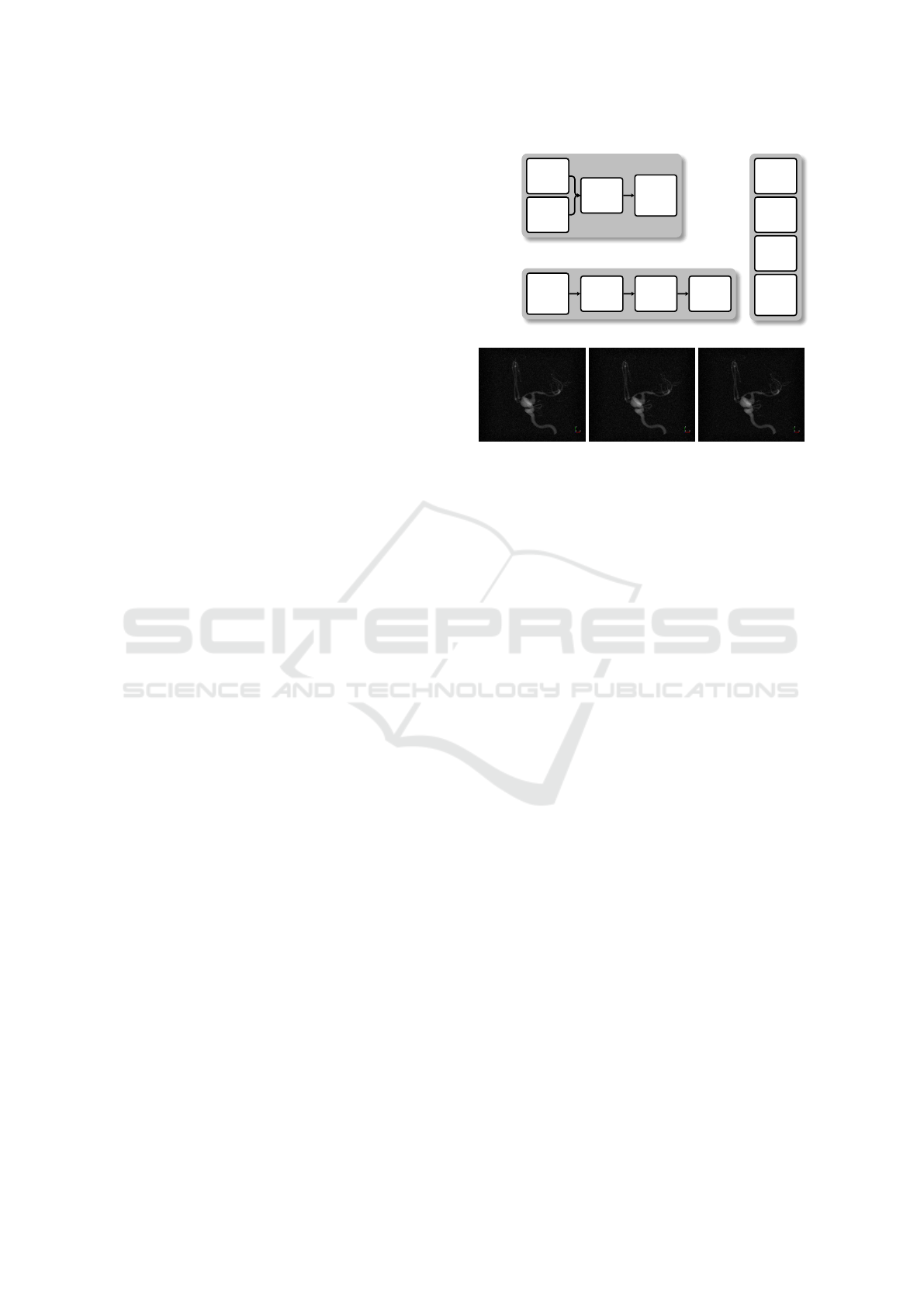
(a)

(b) (c) (d)

Figure 8: (a) Schematic depiction of the order by which the

different artifacts are applied to the dataset in Scenario 2.

(b–d) Visual comparison of order A, B, and C, respectively.

tation tasks, particularly in assessing aneurysm shape

and volume. The detailed and complex arterial struc-

tures make segmentation sensitive to artifacts, and

with only one primary structure of interest, the setup

remains interpretable. This scenario aims to explore

the impact of artifact application order on segmen-

tation outcomes, using four types of image artifacts

(salt and pepper noise, Gaussian noise, cupping, and

ring artifacts). We tested three pipeline conﬁgurations

(Fig. 8 (a)):

Order A. This order replicates the order in which ar-

tifacts naturally occur in real CT imaging, with

Gaussian noise and cupping ﬁrst (as transmission

artifacts), followed by ring (being scanner-based

artifacts) and salt-and-pepper noise (again due to

data transmission) (see Fig. 8 (b)).

Order B. All artifacts are applied in parallel (see

Fig. 8 (c)).

Order C. All artifacts are applied in sequence, with

an arbitrary ordering that is distinct from the other

two for diversity (see Fig. 8 (d)).

In each conﬁguration, artifact parameters re-

mained consistent, though the sequence varied. Vi-

sual analysis of these orders showed slight noise pat-

terns and segmentation differences in ﬁne structures.

To determine an optimal threshold (109 HU) for seg-

mentation, Otsu’s method (Otsu, 1979) was used to

maximize the inter-class variance between the back-

ground and the structure of interest. The same 32 ra-

diomics features were also extracted here for all cases.

The t-SNE analysis displayed ﬁve relatively dis-

tinct clusters, although less well-formed than in the

Investigating the Propagation of CT Acquisition Artifacts along the Medical Imaging Pipeline

759

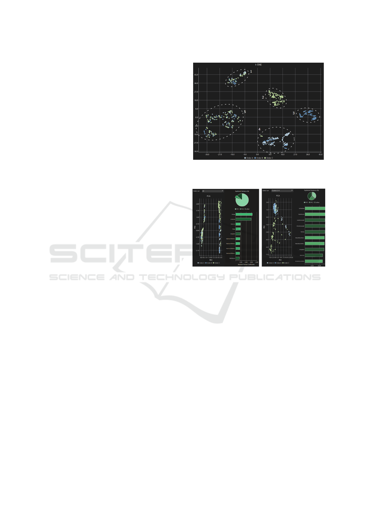
previous scenario (Fig. 9). The algorithm was able

to ﬁnd similarities within ﬁve groups of data points,

albeit they were not as strong as for the ﬁrst sce-

nario. Each cluster included data points from mul-

tiple pipeline groups, which means that some inter-

pipeline-group similarities exist in our data. This is an

expected result because the pipeline groups use iden-

tical artifact parameters. However, we also see differ-

ences caused by the different orders since Clusters 1,

4, and 5 (Fig. 9) contain unequal shares of data points

from each pipeline group. While Clusters 2 and 3 only

contain data points from Order B and C, respectively.

Salt noise was found consistently across intra-group

points, while other artifact parameters varied across

their full range. Additionally, we ﬁnd that the posi-

tion of a data point within a cluster no longer reliably

predicts the values of individual artifact parameters.

This suggests that clustering patterns emerged from

combinations of artifact parameters rather than indi-

vidual ones.

PCA was used to interpret the parameter impacts

on segmentation (Fig. 10). PC1 explained over 80%

of the variance in individual groups, primarily due to

the absence of salt noise (Fig. 10, left; pie chart). We

already determined this factor to be inﬂuential during

the t-SNE analysis. PCA hardly reveals any informa-

tion about the inﬂuence of artifact order because the

separation affects all pipeline groups approximately

the same. Based on the features with the biggest fea-

ture coefﬁcients, we observe that many of our fea-

tures are sensitive to large outliers within the image.

In PC2, which explains only 6.7% of the variance

(Fig. 10, left; pie chart) but is less correlated with

PC1, entropy and uniformity were primary contribu-

tors among the radiomics features. Order C showed

the highest entropy, especially in images with salt

noise, while Order B exhibited the lowest. Order B,

with parallel application, impacts radiodensities less,

and Order A places salt and pepper noise last, reduc-

ing entropy.

Upon looking at the PCA of pipelines with salt

noise (Fig. 10, right), shape features contributed sig-

niﬁcantly to PC1 (Fig. 10, right; pie and bar chart).

Least axis length and minor axis length affect PC1

negatively. Here, these can be interpreted as prefer-

ring a center of mass that aligns better with the center

of the bounding box of a segmentation. This is the

case when the ring artifact affects the region of the

aneurysm strongly because it is the thickest structure

in the image, which can reduce the size of the error

ellipsoid. These quantities stay relatively uniform for

Order B compared to Orders A and C because with

the parallel artifacts of order B, the effects of one ar-

tifact do not inﬂuence the effects of the others.

Figure 9: t-SNE for Scenario 2. Five clusters can be re-

trieved, and are highlighted using dashed ellipses and iden-

tiﬁed via indices.

Figure 10: PCAs for Scenario 2: (left) PCAs between all

orders (A, B, and C), where artifact pipelines without salt

noise are on the left-hand side and pipelines with salt noise

on the right-hand side; (right) PCAs of artifact pipelines

containing salt noise from all orders.

Performance. The generation of the artifact-affected

CT images took 1 hour 57 minutes, most of which

was used for data compression and writing. On the

other hand, feature extraction took only 37 minutes.

The amount of time PCA and t-SNE needed was also

negligible for this example scenario since we had a

similar number of feature values as in Scenario 1. The

relatively large amount of time spent on compression

and writing was necessary because the images have an

anisotropic resolution of 256 pixels along each axis.

Therefore, the ﬁle size of one image was around 100.6

MB, which would have resulted in 76 GB of data but

were compressed to 35.4 GB.

5 DISCUSSION

Flexibility is a strength of our application that is

demonstrated in both use cases. Users are empow-

ered to investigate arbitrary artifact conﬁgurations,

IVAPP 2025 - 16th International Conference on Information Visualization Theory and Applications

760

and they may tailor all settings to the imaging tasks of

their interest. As already mentioned in Sec. 2, there is

limited prior work similar to ours. Therefore, our re-

sults are challenging to contextualize within ﬁndings

from prior research. However, the fact that the results

of our data analysis agree with literature expectations

or are supported by reasonable explanations is already

a positive indication.

Our approach to evaluating CT artifacts has sev-

eral limitations. While the framework effectively

identiﬁes and quantiﬁes standard artifacts, it may not

adequately capture complex artifacts or interactions

between them. For example, compound effects with

the segmentation step are not currently addressed, as

our approach focuses only on the acquisition uncer-

tainties and their propagation through the pipeline. In

the future, it would be valuable to increase the se-

lection of segmentation algorithms and explore the

impact of this choice (as well as its interplay with

the other steps). Additionally, the extension of this

methodology to other imaging modalities is theoreti-

cally possible. Yet, it presents challenges due to the

unique characteristics and types of artifacts associ-

ated with each modality. Moreover, the actual im-

pact of the ﬁndings discussed in Sec. 4 on clinical

decision-making needs a more concrete assessment.

Keeping in mind that the investigated uncertainties

are not the only ones potentially present in an ana-

lytical process (Gillmann et al., 2023; Sacha et al.,

2016), a comprehensive study that includes also the

other types would be necessary. As a future direction,

the framework could integrate a differential analysis

feature to compare selected points in the projected

views with their respective 3D representations. While

the quantitative data and visualizations presented in

the use cases are valuable, evaluating the effective-

ness of our approach in real-world settings with prac-

titioners would be the next step in understanding the

practical implications of our work. For instance, it

would be valuable to evaluate the framework in a set-

ting in which the user learns how uncertainties are

propagated through the medical imaging pipeline.

6 CONCLUSIONS

This work investigated the effects of CT acquisition

artifacts on the subsequent steps and outcomes of the

medical imaging pipeline. Our results indicate that:

• The uncertainty introduced by CT artifacts

impacts segmentation outcomes and feature

extraction—varying by artifact type, order, and

magnitude.

• Our application supports the effective exploration

of the impact of uncertainties on the outcomes of

the medical imaging pipeline.

Our current limitations comprise the choice (and

unexplored effect on the pipeline outcome) of seg-

mentation algorithms and the complexity of artifact

modeling. Addressing these limitations opens inter-

esting directions for future work that are expected to

improve the framework’s generalizability and provide

additional insights into uncertainty propagation.

REFERENCES

Abdi, H. and Williams, L. J. (2010). Principal component

analysis. WIREs Computational Statistics, 2(4):433–

459.

Athanasiou, L. S., Rigas, G., Sakellarios, A., Bouran-

tas, C. V., Stefanou, K., Fotiou, E., Exarchos, T. P.,

Siogkas, P., Naka, K. K., Parodi, O., Vozzi, F., Teng,

Z., Young, V. E., Gillard, J. H., Prati, F., Michalis,

L. K., and Fotiadis, D. I. (2015). Error propagation in

the characterization of atheromatic plaque types based

on imaging. Computer Methods and Programs in

Biomedicine, 121(3):161–174.

Barrett, J. F. and Keat, N. (2004). Artifacts in ct: Recog-

nition and avoidance. RadioGraphics, 24(6):1679–

1691. PMID: 15537976.

Behrens, T., Woolrich, M., Jenkinson, M., Johansen-Berg,

H., Nunes, R., Clare, S., Matthews, P., Brady, M., and

Smith, S. (2003). Characterization and propagation of

uncertainty in diffusion-weighted mr imaging. Mag-

netic resonance in medicine : ofﬁcial journal of the

Society of Magnetic Resonance in Medicine / Society

of Magnetic Resonance in Medicine, 50:1077–88.

Boas, F. E. and Fleischmann, D. (2012). Ct artifacts: Causes

and reduction techniques. Imaging in Medicine,

4:229–240.

Brodlie, K., Osorio, R. S. A., and Lopes, A. (2012). A re-

view of uncertainty in data visualization. In Expand-

ing the Frontiers of Visual Analytics and Visualization,

pages 81–109.

Diwakar, M. and Kumar, M. (2018). A review on ct image

noise and its denoising. Biomedical Signal Processing

and Control, 42:73–88.

Feiner, L. F., Menten, M. J., Hammernik, K., Hager,

P., Huang, W., Rueckert, D., Braren, R. F., and

Kaissis, G. (2023). Propagation and Attribution of

Uncertainty in Medical Imaging Pipelines, page 1–11.

Springer Nature Switzerland.

Gillies, R. J., Kinahan, P. E., and Hricak, H. (2016). Ra-

diomics: images are more than pictures, they are data.

Radiology, 278(2):563–577.

Gillmann, C., Arbel

aez, P., Hern

andez, J. T., Hagen, H.,

and Wischgoll, T. (2017). Intuitive Error Space Explo-

ration of Medical Image Data in Clinical Daily Rou-

tine. In Kozlikova, B., Schreck, T., and Wischgoll, T.,

editors, EuroVis 2017 - Short Papers. The Eurograph-

ics Association.

Investigating the Propagation of CT Acquisition Artifacts along the Medical Imaging Pipeline

761

Gillmann, C., Maack, R. G. C., Raith, F., P

erez, J. F., and

Scheuermann, G. (2023). A taxonomy of uncertainty

events in visual analytics. IEEE Computer Graphics

and Applications, 43(5):62–71.

Gillmann, C., Saur, D., Wischgoll, T., and Scheuermann,

G. (2021). Uncertainty-aware visualization in medi-

cal imaging - a survey. Computer Graphics Forum,

40(3):665–689.

Gravel, P., Beaudoin, G., and de Guise, J. A. (2004). A

method for modeling noise in medical images. IEEE

Transactions on Medical Imaging, 23:1221–1232.

Howard, M., Luttman, A., and Fowler, M. (2014).

Sampling-based uncertainty quantiﬁcation in decon-

volution of x-ray radiographs. Journal of Computa-

tional and Applied Mathematics, 270:43–51. Fourth

International Conference on Finite Element Methods

in Engineering and Sciences (FEMTEC 2013).

Klacansky, P. (2017). Open scivis datasets.

https://klacansky.com/open-scivis-datasets/.

Laidlaw, D. H., Trumbore, W. B., and Hughes, J. F. (1986).

Constructive solid geometry for polyhedral objects.

In Proceedings of the 13th Annual Conference on

Computer Graphics and Interactive Techniques, SIG-

GRAPH ’86, page 161–170, New York, NY, USA. As-

sociation for Computing Machinery.

Lorensen, W. E. and Cline, H. E. (1987). Marching cubes:

A high resolution 3d surface construction algorithm.

In Proceedings of the 14th Annual Conference on

Computer Graphics and Interactive Techniques, SIG-

GRAPH ’87, page 163–169, New York, NY, USA. As-

sociation for Computing Machinery.

Lu, C.-T., Chen, M.-Y., Shen, J.-H., Wang, L.-L., and Hsu,

C.-C. (2018). Removal of salt-and-pepper noise for

x-ray bio-images using pixel-variation gain factors.

Computers & Electrical Engineering, 71:862–876.

Madhura, J. J. and Babu, D. R. R. (2017). An effective hy-

brid ﬁlter for the removal of gaussian-impulsive noise

in computed tomography images. In 2017 Interna-

tional Conference on Advances in Computing, Com-

munications and Informatics (ICACCI), pages 1815–

1820.

Otsu, N. (1979). A threshold selection method from gray-

level histograms. IEEE Transactions on Systems,

Man, and Cybernetics, 9(1):62–66.

Potter, K., Rosen, P., and Johnson, C. R. (2012). From quan-

tiﬁcation to visualization: A taxonomy of uncertainty

visualization approaches. In Dienstfrey, A. M. and

Boisvert, R. F., editors, Uncertainty Quantiﬁcation in

Scientiﬁc Computing, pages 226–249, Berlin, Heidel-

berg. Springer Berlin Heidelberg.

Preim, B. and Botha, C. P. (2013). Visual Computing

for Medicine: Theory, Algorithms, and Applications.

Morgan Kaufmann Publishers Inc., San Francisco,

CA, USA, 2 edition.

Raidou, R. G. (2018). Uncertainty visualization: Recent

developments and future challenges in prostate can-

cer radiotherapy planning. In EuroRV3 2018: EuroVis

Workshop on Reproducibility, Veriﬁcation, and Vali-

dation in Visualization, pages 13–17. The Eurograph-

ics Association.

Reiter, O., Breeuwer, M., Gr

oller, E., and Raidou, R.

(2018). Comparative visual analysis of pelvic organ

segmentations. pages 037–041.

Ristovski, G., Preusser, T., Hahn, H. K., and Linsen, L.

(2014). Uncertainty in medical visualization: Towards

a taxonomy. Computers & Graphics, 39:60–73.

Roy, C. J. and Oberkampf, W. L. (2011). A comprehen-

sive framework for veriﬁcation, validation, and uncer-

tainty quantiﬁcation in scientiﬁc computing. Com-

puter Methods in Applied Mechanics and Engineer-

ing, 200(25):2131–2144.

Sacha, D., Senaratne, H., Kwon, B. C., Ellis, G., and Keim,

D. A. (2016). The role of uncertainty, awareness, and

trust in visual analytics. IEEE Transactions on Visu-

alization and Computer Graphics, 22(1):240–249.

Schlachter, M., Raidou, R. G., Muren, L. P., Preim, B.,

Putora, P. M., and B

uhler, K. (2019). State-of-the-

art report: Visual computing in radiation therapy plan-

ning. In Computer Graphics Forum, volume 38, pages

753–779. Wiley Online Library.

Tian, X. and Samei, E. (2016). Accurate assessment and

prediction of noise in clinical ct images. Medical

Physics, 43(1):475–482.

van der Maaten, L. (2014). Accelerating t-sne using tree-

based algorithms. Journal of Machine Learning Re-

search, 15(93):3221–3245.

van der Maaten, L. and Hinton, G. (2008). Visualizing data

using t-sne. Journal of Machine Learning Research,

9(86):2579–2605.

Wu, Y., Yuan, G.-X., and Ma, K.-L. (2012). Visualiz-

ing ﬂow of uncertainty through analytical processes.

IEEE Transactions on Visualization and Computer

Graphics, 18:2526–2535.

Yucel-Finn, A., Mckiddie, F., Prescott, S., and Grifﬁths, R.

(2023). A Brief History of Time: From the Big Bang

to Black Holes. Elsevier, 1 edition.

Zhang, J. (2021). Modern monte carlo methods for efﬁcient

uncertainty quantiﬁcation and propagation: A survey.

WIREs Computational Statistics, 13(5):e1539.

Zhou, S. K., Greenspan, H., Davatzikos, C., Duncan, J. S.,

Van Ginneken, B., Madabhushi, A., Prince, J. L.,

Rueckert, D., and Summers, R. M. (2021). A re-

view of deep learning in medical imaging: Imaging

traits, technology trends, case studies with progress

highlights, and future promises. Proceedings of the

IEEE, 109(5):820–838.

APPENDIX

The symbols x =

and x

= [

] denote the image

position in all artifact models described below.

Salt and Pepper Noise Artifact

For the salt and pepper noise artifact, we use the fol-

lowing four parameters:

IVAPP 2025 - 16th International Conference on Information Visualization Theory and Applications

762

radiodensity of salt-pixels

radiodensity of pepper-pixels

relative amount of salt-pixels

relative amount of pepper-pixels

where p

+ p

≤ 1.0. The output for all values of the

image is then deﬁned as

out

(x, Ω) =











if Ω = 1

if Ω = 2

(x) if Ω = 3

(1)

with Ω ∼ Categorical



, p

, 1.0 − (p

+ p

)



Gaussian Noise Artifact

The parameters of Gaussian noise artifacts, following

a Poisson distribution, are:

µ mean of Gaussian distribution

σ standard deviation of Gaussian distribution

for the output image

out

(x, T ) = I

(x) + T (2)

with T ∼ N (µ, σ

Cupping Artifact

Our cupping artifacts model uses the following pa-

rameters:

min

minimum relative radiodensity at center

c =





center voxel with maximum shading

Further, we assume that the shading effect increases

linearly towards the center of the artifact to arrive at

the model

out

(x) = I

(x)



min

+ (1.0 − k

min

)

max

− d

)

max



(3)

where d

) =

− c

is the distance from the cen-

ter, and d

max

= max

∈A

) is the maximum dis-

tance from the center to any voxel in the image.

Ring Artifact

The ring artifacts model takes the following parame-

ters:

r inner radius of the ring

w width of the ring

relative radiodensity of the ring voxels

c =





ring center

The output radiodensities are determined by:

out

(x) =

(

(x) if

− c

∈ [r, r + w]

(x) else

(4)

Metal Artifact

Metal artifacts modeling makes two central assump-

tions: (a) There is only one direction of highest atten-

uation and one direction of lowest attenuation, which

is perpendicular to the former, and (b) the shading ef-

fect decreases linearly with the distance when moving

away from the boundaries of the structure on a certain

slice. It takes the following parameters:

min

minimum relative radiodensity adjacent to the

structure in direction of maximum attenuation

l length of effects beginning at structure border

u =





direction of highest attenuation

Before we state our model, let the closest point on an

implicit surface S(x) to a given point on the z-value of

the point be

(x) = argmin

Q∈V

S,z

x − Q

(5)

with V

S,z

= {x ∈ V | w = z ∧ S(x) = 0} being the set of

points on the curve deﬁned by the cross section of the

xy-plane with the structure S at the current z-value.

Then, we determine the output image using

out

(x, S

) =

(

(x) if ∄P

(x)

(x) + R

max,ξ

dis

dir

else

(6)

where ξ is the implicit structure to which the artifact is

applied, R

max,ξ

is the maximum radiodensity observed

within the structure ξ,

dis

= max



0.0, 1.0 −



(7)

is the distance weighting factor with δ = x − P

, and

dir

= k

max



1.0 − 2 (1.0− k

max

) cos



δ · u



(8)

is the direction weighting factor.

Windmill Artifact

Windmill artifacts are modeled with the following pa-

rameters:

max

maximum relative radiodensity adjacent

to the structure on a bright streak

l length of effects beginning at structure border

γ angular width of a single bright streak

φ rotation per slice

The output image is deﬁned by:

out

(x, S

) =

(

(x) if ∄P

(x)

(x) + R

max,ξ

max

dis

dir

else

(9)

where ξ, R

max,ξ

, a

dis

as well as δ conform to the deﬁ-

nitions provided previously for the metal artifact and

dir

= cos



atan2(δ

, δ

) + φ (z − z

min

) +



(10)

is the direction weighting factor.

Investigating the Propagation of CT Acquisition Artifacts along the Medical Imaging Pipeline

763

Motion Artifact

Motion artifacts models take the following parame-

ters:

max

relative radiodensity at the difference region

A linear transformation matrix

Gaussian blur kernel radius

σ Gaussian blur kernel standard deviation

The output image is deﬁned by:

out

(x, S

) =

(

,σ

∗ I

(x) if x ∈ V

(x) else

(11)

where ξ conforms to the deﬁnition provided previ-

ously,

(x) =

x ∈ V



(x) > 0 ∧ S



−1



≤ 0

(12)

is the set of points in the transformation region,

(x) = k

max



−1



(13)

the intensity after transformation, but before blurring,

and Γ

,σ

is the Gaussian kernel used for blurring.

IVAPP 2025 - 16th International Conference on Information Visualization Theory and Applications

764