ShadowScout: Robust Unsupervised Shadow Detection for RGB Imagery
Estephan Rustom
a
, Henrique Cabral
b
, Sreeraj Rajendran
c
and Elena Tsiporkova
d
EluciDATA Lab, Sirris, Bd A. Reyerslaan 80 1030, Brussels, Belgium
Keywords:
Shadow Detection, Unsupervised Learning, Deep Learning, CNN.
Abstract:
Accurate shadow detection and correction are critical for improving image classification and segmentation
but remain challenging due to the lack of well-labeled datasets and the context-specific nature of shad-
ows, which limit the generalizability of supervised models. Existing unsupervised approaches, on the
other hand, often require specialized data or are computationally intensive due to high parameterization.
In this paper, we introduce ShadowScout, a novel, low-parameterized, unsupervised deep learning method
for shadow detection using standard RGB images. ShadowScout is fast, achieves performance compara-
ble to state-of-the-art supervised methods, and surpasses existing unsupervised techniques across various
datasets. Additionally, the model can seamlessly incorporate extra data, such as near-infrared channels, to
enhance shadow detection accuracy further. ShadowScout is available on the authors’ GitHub repository
(https://github.com/EluciDATALab/elucidatalab.starterkits/tree/main/models/shadows).
1 INTRODUCTION
Shadows form an omnipresent element in most cases
of real-life imagery, the result of light blocked by ob-
jects present in the physical world. In recent years, as
the demand for AI-based scene understanding in com-
puter vision has grown, accurately detecting and sub-
sequently correcting shadows has emerged as a sig-
nificant challenge. Shadow regions often have incom-
plete spectral information, lower intensity, and fuzzy
boundaries leading to information loss and poorer
scene representation. This ultimately reduces the per-
formance of image segmentation and classification al-
gorithms (Wang et al., 2017; Vazquez et al., 2008;
Zhang et al., 2014). This is particularly relevant in
the case of remote sensing aerial images, where vege-
tation and infrastructure creates complex shadows of
varying intensity, shape and size (Luo et al., 2019; He
et al., 2022). This underscores the importance of im-
plementing a shadow correction processing step be-
fore image analysis.
A crucial step in the shadow correction process
consists in their detection. While shadow detection is
often addressed using a supervised approach, this re-
quires the availability of ground truth shadow masks
a
https://orcid.org/0009-0008-9075-8654
b
https://orcid.org/0009-0006-9182-0056
c
https://orcid.org/0000-0002-9056-7494
d
https://orcid.org/0009-0003-7202-3471
to train a model, typically deep learning-based, to
carry out the shadow detection. Such approaches face
two major challenges:
• Only a few publicly available, annotated datasets
exist (ISTD (Wang et al., 2018), AISD (Luo et al.,
2020) or CUHK-Shadow (Hu et al., 2021)), and
creating a dedicated labeled dataset requires sig-
nificant time and effort and it is a very costly pro-
cess.
• Images from different contexts show significant
variability in lighting, object types, camera set-
tings, and other factors. Our observation is that
shadow detection models trained on available
datasets lack robustness and struggle to general-
ize to different scenarios.
In view of these limitations, unsupervised shadow
detection methods, where shadow masks are derived
from the images by perceived differences between
shadow and non-shadow regions, offer a promising
alternative, especially when a dedicated model can
be trained for each dataset. However, the complex-
ity of shadows, which vary in intensity, shape, and
texture based on light conditions, object shapes, and
surfaces make unsupervised shadow detection a chal-
lenging task, particularly in deep learning approaches.
Few studies have explored this path(see (Koutsiou
et al., 2024; Zhou et al., 2022)). Several physics-
based models for unsupervised shadow detection ex-
ist, but they often require access to data sources that
Rustom, E., Cabral, H., Rajendran, S. and Tsiporkova, E.
ShadowScout: Robust Unsupervised Shadow Detection for RGB Imagery.
DOI: 10.5220/0013254900003912
Paper published under CC license (CC BY-NC-ND 4.0)
In Proceedings of the 20th International Joint Conference on Computer Vision, Imaging and Computer Graphics Theory and Applications (VISIGRAPP 2025) - Volume 3: VISAPP, pages
657-668
ISBN: 978-989-758-728-3; ISSN: 2184-4321
Proceedings Copyright © 2025 by SCITEPRESS – Science and Technology Publications, Lda.
657

are not always available, such as spectral differences
(Finlayson et al., 2007; Makarau et al., 2011) or ge-
ometric features (Salvador et al., 2004; Wang et al.,
2017). He et al. (2022) propose a physics-based
model using thresholding of the hue (H), saturation
(S), and intensity (I) channels in RGB images, opti-
mized via particle swarm optimization. Though ef-
fective on the AISD, this method is computation-
ally heavy as it optimizes per image, always identi-
fies two groups regardless of shadow presence, under-
performs in highly saturated images, and requires ex-
tensive parameter tuning to adapt to different datasets.
We present here ShadowScout, an unsupervised
deep learning method that processes channels derived
from the HSI color model to infer image-specific
thresholds to determine shadow regions in the image.
The approach addresses the limitations mentioned out
above to make a fast, robust and precise shadow de-
tection method across datasets with images of differ-
ent types. Our key contributions are:
• The separation of the pixels in an image into
shadow and non-shadow groups based on an en-
semble of images, allowing to better capture the
properties of shadows.
• The use of a convolutional neural network (CNN)
for thresholding, reducing the parameterisation
degree of the approach and leveraging the in-
herent capabilities of CNNs to process local
and global image/shadow properties (Krizhevsky
et al., 2012).
• The use of a novel, adapted Calinski-Harabsz met-
ric (Cali
´
nski and Harabasz, 1974) as loss to the
CNN model, which confers the model higher ro-
bustness in the thresholding process.
• The ability to seamlessly extend the model inputs
to extra data sources, such as the near-infrared
band, for increased performance.
2 RELATED WORKS
The shadow detection problem involves assigning bi-
nary value to each pixel in an image, identifying
shaded regions as the positive class. Shadow detec-
tion methods are broadly categorized into supervised
and unsupervised methods: while supervised meth-
ods rely on annotated datasets to learn abstract image
features for binary classification, unsupervised meth-
ods make use of intrinsic physical and statistical prop-
erties of shadow regions to separate them from non
shadow regions (He et al., 2022).
Supervised methods generally achieve the best
performance but often struggle to generalize beyond
their training datasets. In contrast, unsupervised
methods are valuable when labeled datasets are un-
available or when annotating data is impractical due
to the time and effort involved. The BDRAR model
(Zhu et al., 2018), a supervised approach, has shown
notable outcomes by using a bidirectional feature
pyramid architecture and a recurrent attention resid-
ual module to enhance shadow details and reduce
false detections.
In another study, Luo et al. (2020) used an
encoder-decoder residual structure to capture shadow
features across different layers, with deep supervision
enhancing performance. This method showed impres-
sive results on the CUHK-Shadow dataset. More re-
cently, Wang et al. (2024) introduced SwinShadow,
a transformer-based approach focusing on adjacent
shadows. The architecture includes encoding with
Swin Transformers, decoding with deep supervision
and double attention modules, and feature integra-
tion via multi-level aggregation, designed to improve
shadow-object distinction.
Luo et al. (2019) proposed a method to correct in-
consistencies between shadow and non-shadow areas
through separated illumination correction, focusing
on shadow-related illumination. This approach uses
a spatially adaptive weighted total variation model to
derive shadow-related illumination and shadow-free
reflectance, enabling object-oriented illumination cor-
rection. Its effectiveness was validated on an aerial
images dataset through visual inspection.
Zhu and Woodcock (2012) introduced Fmask for
detecting clouds and shadows in Landsat imagery us-
ing Top of Atmosphere (TOA) reflectance and Bright-
ness Temperature (BT). Fmask creates a cloud proba-
bility mask based on physical properties, temperature,
spectral variability, and brightness, and predicts cloud
shadows by analyzing the Near Infrared (NIR) band
along with satellite viewing and illumination angles.
In Sun et al. (2019), the authors developed a
combinational shadow index (CSI) using Sentinel-2A
Multispectral Instrument (MSI) images by combining
the shadow enhancement index, normalized differ-
ence water index, and the NIR band. He et al. (2022)
introduced DLA-PSO, an unsupervised shadow de-
tection algorithm. DLA-PSO is a customized Parti-
cle Swarm Optimization (PSO) algorithm that uses
Otsu’s method as its fitness function.
Ghandour and Jezzini (2019), presented their
SMS unsupervised algorithm which relies on thresh-
olding the value component of the HSV color space
using Otsu’s method in order to differentiate between
shadow and non shadow regions. Such method has a
limitation because a lot of valuable information is lost
by eliminating the hue and saturation components.
VISAPP 2025 - 20th International Conference on Computer Vision Theory and Applications
658

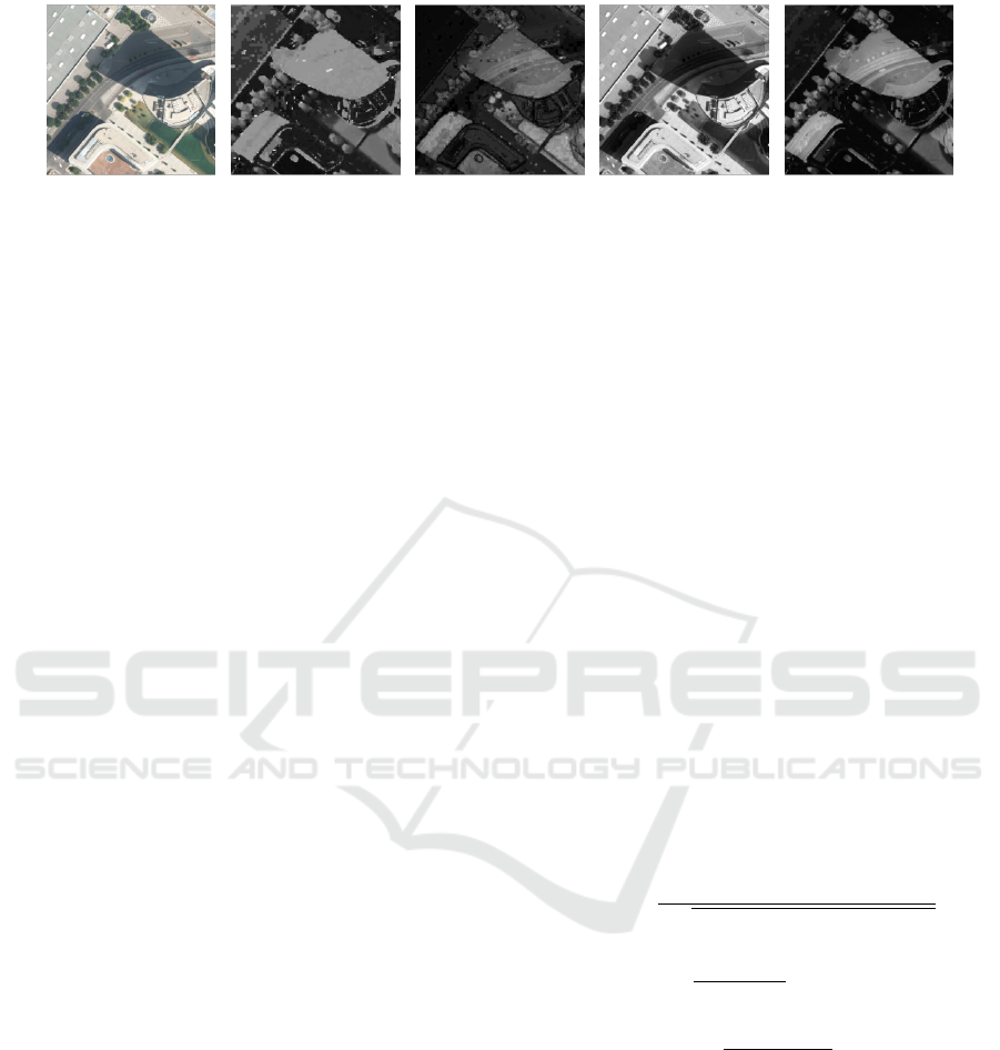
(a) Original image. (b) H channel. (c) S channel. (d) I channel. (e) HI channel.
Figure 1: Example of an aerial image from the AISD dataset Luo et al. (2020) to show the importance of the HI, I and S
channels.
The method only measures the pixels’ similarity to
black and white colors.
Chung et al. (2008) proposed another unsuper-
vised algorithm for shadow detection called Suc-
cessive Thresholding Scheme (STS). This algorithm
separates pixels between shadow and non shadow
based on a interative thresholding scheme. Although
this method demonstrated promising results, it is
time-consuming, due to its iterative and sequential
per-image processes, extensive pixel-wise operations,
high memory usage for intermediate results, and lim-
ited parallelization.
Unsupervised methods, despite good results, face
notable challenges. They depend on specific data
types that may not always be available and require
significant parameter tuning, which demands deep
domain expertise and extensive experimentation, es-
pecially with new datasets. Moreover, optimizing
parameters is computationally intensive, and shadow
characteristics often vary by context, limiting the gen-
eralizability and adaptability of these methods across
different scenarios.
3 METHODOLOGY
Here we provide a detailed explanation of our unsu-
pervised framework for shadow detection, ShadowS-
cout, that optimizes thresholding across transformed
RGB images in the HSI color space, where shad-
ows are better characterized. A convolutional neu-
ral network (CNN) is used to dynamically determine
channel-specific thresholds, separating shadowed and
non-shadowed pixels. The model uses a custom loss
function based on an adapted Calinski-Harabasz in-
dex to maximize the clustering quality of shadow re-
gions, ensuring an optimal separation. This section
covers the selection and processing of model inputs,
the architecture, and the custom loss function.
3.1 Choice of Model Inputs
RGB channels are not directly suitable for the detec-
tion of shadows because they do not effectively sep-
arate brightness from color information. Shadows
primarily cause variations in luminance rather than
color, which means that in RGB space, shadows can
appear similar to other dark regions unrelated to shad-
ows, leading to poor discrimination. Additionally,
RGB channels are sensitive to illumination changes,
making it difficult to distinguish shadows from other
low-light areas without specific features that are in-
variant to lighting conditions. As such, and based on
the work by He et al. (2022), the original RGB image
is first converted to the HSI color space which con-
sists of hue (H), saturation (S) and intensity (I). The
conversion is obtained using the following formulas
(Gonzalez, 2009):
H =
(
θ, B ≤ G
360 − θ, B > G
(1)
θ = arccos
(R − G) +(G − B)
2
p
(R − B)
2
+ (R − B)(G − B)
!
(2)
S = 1 −
3
R + G + B
min(R, G,B) (3)
I =
(R + G +B)
3
(4)
In order to avoid Gaussian noise, which can af-
fect shadow detection, a Gaussian filtering is applied
on the three channels separately (Kotecha and Djuric,
2003).
The HSI channels are more effective for captur-
ing shadow effects than RGB channels. Shadows
generally exhibit lower intensity values (Liu et al.,
2011) and higher hue values due to reduced direct
light and increased indirect or ambient light. This ef-
fect can be explained using the Phong illumination
model (Li et al., 2015). While shadows are typi-
cally linked to lower saturation (Saha and Chatterjee,
ShadowScout: Robust Unsupervised Shadow Detection for RGB Imagery
659

2017), this relationship can vary in certain contexts,
such as aerial imagery, where atmospheric Rayleigh
scattering causes shadows to exhibit higher saturation
values (Polidorio et al., 2003).
The HSI channels, however, still struggle to distin-
guish shadows from some other ambiguous contexts,
such as vegetation, which also show high hue and low
intensity values, as seen in figure 1b and 1d. To fur-
ther distinguish from these confounding factors and
enhance the difference between the hue and intensity
channels, Chung et al. (2008) introduced the HI chan-
nel to replace the H channel as input to the model,
which is calculated from dividing the hue channel
by the intensity channel. HI values are greatest in
shadow regions, but are low in situations with similar
H and I values, such as vegetation, as seen in Figure
1e.
Input channels are normalized prior to being fed
to the model, to ensure consistency and a smoother
learning. The I and S channels are normalized with a
min-max function.
Given that the HI channel can assume extremely
large values when I is very low, leading to right-
skewed distributions, its values are transformed fol-
lowing Equation 5:
HI =
(
x if x < 1
1 + log(x) if x ≥ 1
(5)
where x represents the normalized pixel value of
the HI channel.
To further mitigate the impact of a skewed distri-
bution, the maximum value in the min-max normal-
ization function is replaced with the 95
th
percentile
and values clipped to 1.
3.2 Unsupervised Model for Threshold
Optimization
The ShadowScout model is based on an unsuper-
vised Convolutional Neural Network (CNN) designed
to detect shadows by deriving image-specific thresh-
olds across the HI, I, and S channels. ShadowS-
cout processes each channel through a series of con-
volutional layers, followed by fully connected layers
that output channel-specific thresholds. An objective
function, based on the cluster separation Calinski-
Harabasz metric (Cali
´
nski and Harabasz, 1974), is
used as loss to the model, guiding it to define thresh-
olds which will lead to the best separation of the pix-
els, across the different input channels, into shadow
and non-shadowed regions.
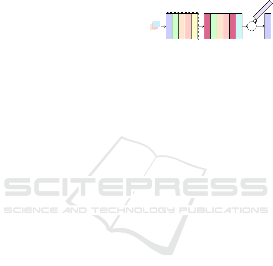
The flexibility of ShadowScout’s architecture, in-
cluding its ability to handle various image shapes and
H-I, I and S
Conv 2D
BatchNorm 2D
ReLU
Dropout 2D
MaxPool 2D
x3
Linear layer
BatchNorm 1D
ReLU
Dropout 1D
Linear layer
Sigmoid
L
CHI
Channel weights
Thresholds
Figure 2: Model architecture with HI, I and S channels as
inputs
adapt its thresholds dynamically, makes it a robust
tool for shadow detection in diverse imaging contexts.
The learnable thresholds and channel weights further
enhance its adaptability, allowing the model to gener-
alize well across different datasets and lighting condi-
tions.
3.2.1 Model Overview
ShadowScout employs a Convolutional Neural Net-
work (CNN) for shadow detection, leveraging the
proven effectiveness of CNNs in image process-
ing. CNNs excel at recognizing patterns and extract-
ing hierarchical features from images, making them
ideal for pixel-level classification tasks (LeCun et al.,
2015). In this framework, ShadowScout is designed
to analyze three channels derived from RGB images,
using the CNN to extract relevant features that distin-
guish between shadowed and non-shadowed regions.
The architecture of ShadowScout is configured to
maximize the model’s ability to detect shadows across
various scales and conditions. It begins with three
convolutional layers, each followed by ReLU activa-
tion to introduce non-linearity, batch normalization to
stabilize learning, dropout to prevent overfitting, and
max-pooling to reduce spatial dimensions while in-
creasing feature map depth. This combination allows
the network to focus on essential features while main-
taining computational efficiency.
The kernel sizes for the convolutional layers are
chosen dynamically, to ensure they cover ±3 stan-
dard deviations around the given sigma, allowing the
model to adapt to different shadow scales and image
resolutions. After feature extraction, the output is flat-
tened and passed through fully connected layers that
continue to refine the feature representation. These
layers also include batch normalization, ReLU activa-
tion, and dropout, ensuring that the network remains
robust and generalizes well to unseen data.
In the final stage, the network outputs threshold
values for each input channel, designed to separate
shadowed pixels from non-shadowed ones. A sig-
moid function is applied to ensure these thresholds
remain within a valid range. Additionally, Shad-
owScout learns channel-specific weights, which are
VISAPP 2025 - 20th International Conference on Computer Vision Theory and Applications
660

constrained within a specified range, adding further
adaptability to different types of input data.
The model is trained in an unsupervised manner,
utilizing a loss function tailored to maximize the sepa-
ration between shadow and non-shadow regions. This
approach not only enhances the model’s flexibility but
also allows it to perform effectively across a variety of
datasets and conditions, making ShadowScout a ro-
bust tool for shadow detection in diverse image pro-
cessing tasks. The overview of the model architecture
is presented in Figure 2.
3.2.2 Shadow and Non-Shadow Pixel Separation
Shadow Mask Definition. The custom loss function
is designed to facilitate the separation of pixels into
shadow and non-shadow regions while addressing
the non-differentiability introduced by binary shadow
masks. To enable gradient-based optimization, the
masks are converted into continuous values, dynami-
cally adjusted for each channel depending on whether
higher (as in the HI channel) or lower values (as in
the I channel) are indicative of shadows, as follows
(Equation 6):
m(x, θ) = σ(ρ(x −θ)), (6)
where m(x, θ) is the shadow mask for input x given
threshold θ, σ is a sigmoid function, which normal-
izes thresholds between 0 and 1 and ρ is either set to
1 or -1 according to the channel input - channels with
higher values associated to shadows have ρ = 1, oth-
erwise ρ = −1.
As mentioned previously, the relationship be-
tween the S channel and shadows is ambiguous,
depending on certain factors such as atmospheric
Rayleigh scattering. To determine, for a given dataset,
how image saturation relates to shadows, the Pearson
correlation between the HI and the S channel is cal-
culated. This follows the assumption that shadows
exhibit higher HI values (from a sample of 1600 im-
ages across the six datasets with ground truth consid-
ered here, 98.3% exhibit a positive Pearson correla-
tion between the HI value and shadow pixels). Con-
sequently, ρ is set to 1 if the correlation to the HI
channel is positive and to -1 otherwise. This step is
reproduced for all remaining input channels for con-
sistency purposes and to facilitate the inclusion of ex-
tra data sources as inputs.
The final mask is derived by initially setting a
combined mask to that of the HI channel and sub-
sequently iteratively combining the individual masks
from each channel with it. In order to maximize gra-
dient updates from the loss, how masks are combined
depends on the ρ parameter of each channel. The final
mask M is computed as follows:
M
combined
=
(
max(M
combined
, M
c
), if ρ
c
> 0
min(M
combined
, M
c
), if ρ
c
≤ 0
(7)
where M
combined
is continuously updated while iterat-
ing over the different channel masks M
c
.
Weighted Channels Computation. Certain chan-
nels exhibit greater discriminative power for shadow
detection, particularly the HI channel, as illustrated
in Figure 1 and demonstrated by He et al. (2022).
To enhance the model’s robustness, channel-specific
weights are introduced as learnable parameters within
the model (see section 3.2.1). Each channel input is
subsequently multiplied by its corresponding weight,
allowing the model to adaptively emphasize the most
relevant channels for shadow detection during train-
ing. The learning of these weights follows a delayed
and transient schedule, with no learning occurring
during the initial 20 epochs, followed by 15 epochs
of active learning. This strategy permits the fine-
tuning of other network parameters before the channel
weights, which have significant influence on the loss
function, are adjusted. The transient nature of this
learning phase is intended to prevent overfitting and to
ensure that the network prioritizes the accurate learn-
ing of channel thresholds. This approach mitigates
the risk of premature weight adjustment, thereby fos-
tering more effective and balanced learning across the
network.
Adapted Calinski-Harabasz Index. The final mask
and the weighted channels are combined as follows:
Flattened Mask: M ∈ R
p×1
,
Flattened Channels: C ∈ R
p×c
,
(8)
where p and c represent the number of pixels and
channels respectively.
The Calinski-Harabasz index is then computed us-
ing these flattened tensors. This index, introduced by
Cali
´
nski and Harabasz (1974), evaluates how well a
clustering algorithm segregates data points into dis-
tinct clusters. The index is calculated as follows:
b =
K
∑
k=1
n
k
∥c
k
− c∥
2
(9)
w =
K
∑
k=1
n
k
∑
i=1
∥d
i
− c
k
∥
2
(10)
h =

b
K − 1

w
N − K

, (11)
where h is the Calinski-Harabasz index, b represents
the between-cluster sum of squares, w the within-
cluster sum of squares, K the number of clusters (set
to 2 for shadow and non-shadow separation), N the
ShadowScout: Robust Unsupervised Shadow Detection for RGB Imagery
661

total number of data points, c the global centroid, n
k
the number of points in cluster k, c
k
the centroid of
cluster k, and d
i
the i
th
data point.
The shadow mask allows for the separation of pix-
els into two groups. The Calinski-Harabasz index
measures clustering quality by comparing the vari-
ance between groups to the variance within groups.
The optimization aims to maximize this index, ensur-
ing a clear and compact separation between shadow
and non-shadow regions.The resulting negated index
L
CHI
is used as the model loss after adding L
1
and L
2
regularization, which is minimized during the training
process:
L
CHI
= −median(log(h(X
f
, M
f
))), (12)
where X
f
represents the flattened channel inputs,
and M
f
represents the flattened combined mask men-
tioned in 7. The median is considered because it is
robust to outliers and represents well the central ten-
dency of skewed data.
3.3 Mask Generation and Evaluation
Metrics
In order for the predicted shadow masks to be com-
pared to their ground truth counterparts, channel-
specific continuous masks are converted to binary
via channel-specific thresholding, following a simi-
lar convention for the threshold direction as laid out
in section 3.2.2.
As mentioned in section 3.2.1, other than finding
the right threshold for pixel separation for each in-
put channels, the model also learns to find the optimal
channel weight to maximize the learning. Therefore,
the masks of the different channels is combined fol-
lowing:
M
′
=
∑
i

µ
i
·
ω
i
∑
i
ω
i

, (13)
where M
′
represents the combined mask, µ represents
the thresholded channel mask and ω represents its re-
spective learned channel weight for the i
th
channel.
M
′
is converted into a binary mask by setting all the
continuous pixel values greater than 0.5 to 1 and the
values smaller than 0.5 to 0.
To assess the model’s fit, we use three metrics: the
Fβ score, balanced error rate (BER) (Vicente et al.,
2016), and Fβ
ω
score (Margolin et al., 2014), a vari-
ation of F1 that addresses its main shortcomings.
BER =
1
2
· (
FP
T N + FP
+
FN
FN + T P
), (14)
Fβ
ω
= (1 +β
2
)
P
ω
· R
ω
(β · P
ω
) + R
ω
, (15)
where FP, T N, FN, T P, P and R represent the
false positives, true negatives, false negatives, true
positives, precision and recall respectively.
The weighted Fβ
ω
measure is ideal for comparing
shadow detection results against ground truth because
it accounts for the varying importance of detection er-
rors, unlike traditional Fβ measures that treat all er-
rors equally. By incorporating weights that consider
the spatial relationship and significance of errors, es-
pecially near important regions like boundaries, the
weighted Fβ
ω
measure provides a more accurate and
meaningful evaluation of shadow detection perfor-
mance, better reflecting the practical needs of the task.
β
2
is chosen to be equal to 1, therefore for simplicity,
throughout the paper, the Fβ and Fβ
ω
scores will be
to renamed F1 and F1
ω
scores respectively.
4 DATASETS
4.1 AISD
In order to showcase the model’s results, the widely
used public dataset for aerial remote sensing imagery,
AISD (Luo et al., 2020) is used as benchmark. This
dataset is composed of images from 5 different cities
in the world with different characteristics, varying in
terms of their urban and others are rural content. This
ensures a fair representation of different scenarios,
such as presence of large infrastructures, like roads
and buildings, but also natural elements, such as veg-
etation. The dataset has 412 training images, 51 val-
idation images and 51 testing images with a spatial
resolutions of 0.3 m.
4.2 CUHK-Shadow
To further test the model’s robustness, we used
five additional non-aerial datasets from the CUHK-
Shadow dataset (Hu et al., 2021): CUHK-
KITTI, CUHK-MAP, CUHK-ADE, CUHK-USR,
and CUHK-WEB. CUHK-KITTI contains 1941 train-
ing, 277 validation, and 555 testing images from road-
side scenes (Geiger et al., 2012). CUHK-MAP has
1116 training, 159 validation, and 319 testing images
from remote-sensing and street-view images. CUHK-
ADE consists of 793 training, 113 validation, and 226
testing images of shadows from buildings (Zhou et al.,
2017). CUHK-USR includes 1711 training, 245 vali-
dation, and 489 testing images of people and objects
(Hu et al., 2019). CUHK-WEB, sourced from Flickr,
has 1789 training, 255 validation, and 511 testing im-
ages.
VISAPP 2025 - 20th International Conference on Computer Vision Theory and Applications
662

The different datasets tested contain images with
different properties, taken in different scenarios. No-
tably, the proportion of shadows in an image also
varies considerably: the AISD and the CUHK-USR
datasets have a median shadow pixel proportion of
0.2, while the other datasets have a median shadow
pixel proportion between 0.37 and 0.51. Addition-
ally, the maximum shadow pixel proportion for the
AISD dataset is 0.49 while the others have a maxi-
mum above 0.9. These aspects demonstrate the ro-
bustness of the ShadowScout model and its capability
to, without the need for labelled data, detect shadows
with great accuracy.
4.3 Near-Infrared Band
To further demonstrate the model’s versatility in
utilizing additional image bands for shadow detec-
tion, we employed orthorectified satellite images with
0.25m resolution from the Belgian Walloon region
1
,
provided by the Service Public de Wallonie
2
. These
images cover an area of 2000m by 2000m which were
divided into 200m by 200m tiles with a resolution of
402x420 pixels. This dataset includes 4-band images,
namely the RGB channels plus a near-infrared band
(NIR), which is particularly effective in distinguish-
ing shadow regions (R
¨
ufenacht et al., 2013).
All images across all datasets were rescaled to
512 × 512 pixels.
5 RESULTS
Although the model is unsupervised, our experiments
followed a traditional supervised methodology, divid-
ing the dataset into training, validation, and testing
splits, ensuring that our results are directly compara-
ble to those of previous methods. However, in practi-
cal applications, the unsupervised nature of the model
allows for training on the entire dataset without the
risk of overfitting, making it highly adaptable and ef-
ficient for real-world scenarios.
For post processing the shadow masks, small low-
brightness objects in non-shadow areas, e.g., dark col-
ored car on the street, are removed by applying a spa-
tial lower limit, and bright small objects in shadow
areas, e.g., light colored water tank on the roof, are
removed by applying mathematical morphology (He
et al., 2022).
1
https://geoportail.wallonie.be
2
https://spw.wallonie.be
5.1 Implementation
The ShadowScout model was implemented using Py-
Torch on a partitioned Nvidia A100 GPU with 80
GB of memory, configured in a Multi-Instance GPU
(MIG) mode, allocating 40 GB to each instance. The
model was trained for up to 200 epochs or until no im-
provement was observed over 40 epochs, with batch
sizes of 15 and 10 for training and validation, respec-
tively. The learning rate for the threshold was set to
1e
−4
and for the channel weights to 1e
−3
. Training
duration ranged between 45 minutes for the AISD
and 2.5 hours for the CUHK-ADE datasets. Cus-
tom weight initialization strategies, set to 0.5 by de-
fault, were employed to ensure stable training from
the start.
5.1.1 Benchmark Models
The ShadowScout model was benchmarked against
a range of well-established unsupervised and super-
vised learning methods commonly used for shadow
removal. The unsupervised methods included a
thresholding approach based on converting the image
from RGB to the C1C2C3 color space (Gevers and
Smeulders, 1999), the spectral ratio of hue to intensity
(SRHI) (Tsai, 2006), the histogram threshold detec-
tion (HTD) method (Zhao and Bao, 1994), a method
utilizing the normalized-blue index (NB) (Zerbe and
Liew, 2004), and the DLA-PSO algorithm (He et al.,
2022). All unsupervised methods were applied with
Otsu’s thresholding (Otsu et al., 1975), by minimizing
intra-class variance and maximizing inter-class vari-
ance between the foreground and background pixel
intensities, and Gaussian filtering was used on inputs
to maintain consistency with our approach. The su-
pervised models evaluated were BDRAR (Zhu et al.,
2018) and U-Net (Ronneberger et al., 2015).
5.2 AISD Dataset
Our ShadowScout model achieved a high perfor-
mance on the AISD dataset, with an overall median
F1 score and F1
ω
scores of 0.837 and 0.901 re-
spectively which are comparable to the best results
achieved by supervised and unsupervised state of the
art techniques as seen in Table 1. Notably, the F1
ω
scores, which account for the spatial distribution of
the errors, show an improvement with respect to the
DLA-PSO. Given the way this metric is constructed,
which penalizes errors according to their spatial dis-
tribution, this suggests that the ShadowScout method
is less likely to make false positive errors in regions
of the image far away from shadow regions.
ShadowScout: Robust Unsupervised Shadow Detection for RGB Imagery
663

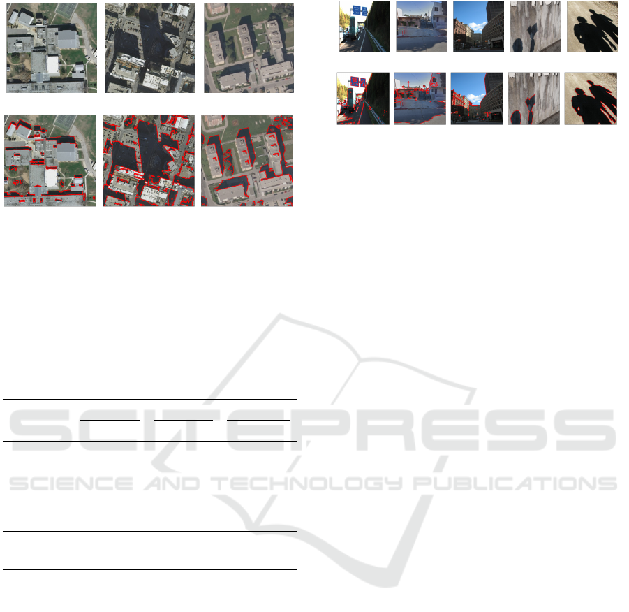
(a) (b) (c)
(d) (e) (f)
Figure 3: AISD shadow detection examples.
Figure 3 shows some examples of shadow detec-
tion from the test dataset. The first row, represents
the original images while the second row shows the
detected shadows using a red contour. Note the well
defined shadow contours irrespective of their size and
context.
Table 1: Comparative evaluation of different methods on
AISD. Models with † are supervised methods.
Methods
F1 score F1
ω
score BER
mean median mean median mean median
C1C2C3 0.642 0.681 0.688 0.719 20.259 18.917
SRHI 0.422 0.516 0.592 0.564 28.599 15.669
HTD 0.560 0.566 0.566 0.570 22.031 21.660
NB 0.738 0.808 0.808 0.894 15.680 13.494
DLA-PSO 0.819 0.845 0.866 0.892 10.985 10.462
ShadowScout 0.815 0.837 0.875 0.901 11.025 10.876
BDRAR
†
0.853 0.858 0.861 0.867 5.449 5.346
U-Net
†
0.901 0.904 0.939 0.945 6.152 6.137
5.3 CUHK-Shadow Dataset
One of the key strengths of the ShadowScout ap-
proach is its robustness and capability to accurately
identify shadows across a wide variety of images,
regardless of their quality or the context in which
they were captured. This versatility was demonstrated
through an evaluation on the CUHK-Shadow dataset,
which comprises five distinct datasets with varying
characteristics. ShadowScout consistently outper-
formed the DLA-PSO (Table 2), except for CUHK-
USR, and, in some instances, even surpassed the per-
formance of the supervised deep learning methods
mentioned earlier. Additionally, ShadowScout out-
performs the other statistical methods by a a large
margin except the HTD which outperforms our model
in all datasets except CUHK-KITTI.
(a) KITTI (b) MAP (c) ADE (d) USR (e) WEB
(f) KITTI (g) MAP (h) ADE (i) USR (j) WEB
Figure 4: CUHK-Shadow shadow detection examples.
For instance, in datasets characterized by signifi-
cant variability, such as CUHK-MAP, CUHK-USR,
and CUHK-WEB (see Section 4.2 and Hu et al.
(2021)), ShadowScout achieved median F1
ω
scores
of 0.7, 0.71, and 0.74, respectively. These results
highlight the model’s ability to generalize effectively
across diverse image types and conditions.
Figure 4 illustrates examples of shadow detection
in CUHK-shadow datasets. The first row displays the
original images, while the second row shows the de-
tected shadows marked with a red contour. Notably,
even in challenging scenarios where shadows occupy
a large portion of the image, such as in CUHK-
KITTI and CUHK-MAP, ShadowScout successfully
captures most shadow regions with minimal errors,
e.g. windows, signs are considered as shadow. This
demonstrates the model’s precision and reliability,
even in complex imaging conditions.
5.4 Extension with Near-Infrared
Channel
ShadowScout is designed to incorporate additional in-
puts beyond the HI, I and S channels derived from
standard RGB images. To demonstrate this flexibil-
ity, we trained the model on a 4-band orthorectified
satellite dataset, which includes a near-infrared (NIR)
channel. The NIR channel is known to highlight dif-
ferences between shadowed and non-shadowed re-
gions, especially in the presence of vegetation, which
has high reflectance in the NIR spectrum (Zhou et al.,
2021). This ability to incorporate additional spectral
information enhances the model’s shadow detection
performance in complex environments. The model
seamlessly integrates the NIR band without requir-
ing additional parameterization, producing an extra
shadow threshold. This additional shadow mask is
combined with the RGB-based masks to create the fi-
nal output. In the absence of ground truth data, we
provide a qualitative assessment.
Figure 5 compares shadow detection using the de-
fault input channels alone (middle row) versus inputs
+ NIR (bottom row). The inclusion of the NIR band
VISAPP 2025 - 20th International Conference on Computer Vision Theory and Applications
664

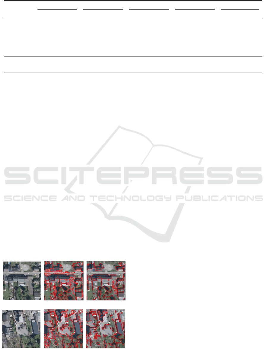
Table 2: Median comparative evaluation on all CUHK-Shadow datasets. Models with † are supervised methods.
Methods
CUHK-KITTI CUHK-MAP CUHK-ADE CUHK-USR CUHK-WEB
F1 F1
ω
BER F1 F1
ω
BER F1 F1
ω
BER F1 F1
ω
BER F1 F1
ω
BER
C1C2C3 0.551 0.613 51.989 0.517 0.569 49.148 0.417 0.470 55.723 0.500 0.553 36.296 0.459 0.555 50.321
SRHI 0.439 0.596 35.928 0.521 0.668 33.280 0.150 0.273 50.000 0.602 0.704 26.337 0.175 0.358 50.000
HTD 0.856 0.859 17.772 0.790 0.807 16.471 0.803 0.819 15.327 0.867 0.889 6.706 0.837 0.866 13.040
NB 0.593 0.666 41.163 0.480 0.552 49.081 0.403 0.476 53.804 0.523 0.556 35.761 0.457 0.553 47.234
DLA-PSO 0.381 0.607 37.498 0.458 0.653 35.203 0.356 0.546 41.471 0.653 0.750 23.051 0.387 0.535 46.309
ShadowScout 0.836 0.902 14.024 0.609 0.698 28.003 0.768 0.820 17.074 0.604 0.712 27.407 0.610 0.745 27.680
BDRAR
†
0.852 0.877 15.010 0.656 0.727 25.847 0.644 0.713 24.895 0.689 0.731 19.700 0.720 0.769 21.045
U-Net
†
0.877 0.903 11.004 0.581 0.699 29.700 0.648 0.760 25.193 0.593 0.688 27.846 0.687 0.777 23.163
enhances shadow detection precision, yielding tighter
boundary detection and reducing false positives, es-
pecially around vegetation and dark objects like roofs.
These results underscore the versatility of ShadowS-
cout, which can integrate additional datasets to further
refine its performance.
6 DISCUSSION
The HSI color space separates the chromatic content
(hue and saturation) from the intensity of the color,
making it ideal for tasks where the distinction be-
tween color and light intensity is important, such as in
shadow detection. ShadowScout is designed to flex-
ibly leverage this information, enabling it to adapt to
different image types. This adaptability is demon-
strated by its high performance on the seven different
datasets reported in this paper. A key aspect of this
success is the CNN’s ability to identify patterns and
features from images: training on a group of images
enables it to derive image type and quality-specific
information, while learning to define image-specific
shadow thresholds.
In addition, the model’s flexibility is enhanced by
statistically determining each channel’s association
(a) Example 1 (b) 3 bands (c) 4 bands
(d) Example 2 (e) 3 bands (f) 4 bands
Figure 5: Shadow detection examples with 4 bands.
with shadows and setting channel weights as param-
eters. This allows the influence of each channel on
shadow detection to be learned automatically for each
dataset.
The design of the loss function allows the model to
find optimal thresholds per channel. He et al. (2022)
used the interclass variance of the shadow mask on
the grayscale images to evaluate the degree of sep-
aration. However grayscaling reduces the image to
intensity variations and loses critical color informa-
tion. As a result, this measure fails to properly assess
the degree of separation in shadow content of the two
groups of pixels. ShadowScout, on the other hand,
uses the Calinski-Harabasz index, which is an effi-
cient metric to measure the degree of separation of
two groups, widely used in clustering algorithms. We
adapted this index to weigh all channels used by the
CNN to predict the shadow thresholds, which ensures
that the separation is optimized based on the highly
informative channels fed to the model.
The DLA-PSO method described in He et al.
(2022), along with the other traditional methods dis-
cussed in Section 5, operates on individual images
by attempting to classify pixels into two categories:
shadow and non-shadow. However, this approach can
be ineffective when an image inherently lacks one of
these categories. In contrast, ShadowScout is trained
on the entire dataset, enabling it to generate more ro-
bust thresholds. As a result, ShadowScout can ef-
fectively handle cases where an image contains only
a single category, such as fully shadowed images or
those entirely without shadows, by clustering all pix-
els into a single cohesive group.
In benchmark testing, ShadowScout was outper-
formed by supervised models by a very small margin,
with a median F1
ω
score difference of no more than
0.03. While the HTD method achieved slightly better
results on four of the five CUHK-Shadow datasets,
this performance can be partly attributed to its per-
image processing approach, which makes it less af-
fected by the diversity within individual datasets.
ShadowScout: Robust Unsupervised Shadow Detection for RGB Imagery
665

Nevertheless, ShadowScout’s consistent performance
across diverse datasets highlights its robustness as an
unsupervised shadow detection method.
Finally, ShadowScout demonstrates exceptional
speed: generating a shadow mask for an image us-
ing a pre-trained model takes a median time of only 5
milliseconds. This performance is significantly faster
than alternative unsupervised methods, which typi-
cally rely on computationally expensive arithmetic or
optimization operations (He et al., 2022). ShadowS-
cout’s efficiency makes it highly suitable for large-
scale or real-time applications, providing a substantial
advantage over existing unsupervised shadow detec-
tion techniques.
However, a limitation of ShadowScout is that it
requires both training and inference on datasets with
similar image types and properties. The relationships
between channel values and shadows, as well as chan-
nel weights, are learned parameters specific to the
dataset rather than individual images. This limitation
likely contributed to the lower performance on the
CUHK-MAP dataset (median F1
ω
of 0.698), which
contains a mix of satellite and mobile camera images.
Notably, even the supervised models struggled with
this dataset, highlighting the challenges posed by high
variability in image types. Additionally, ShadowS-
cout encounters challenges with diverse datasets con-
taining randomly selected images, such as CUHK-
USR and CUHK-WEB, which include both indoor
and outdoor scenes. In such datasets, the relationship
between the saturation channel and shadow regions
varies significantly, making ShadowScout less effec-
tive.
7 CONCLUSION
This paper introduces ShadowScout, a novel unsu-
pervised deep learning method for shadow detec-
tion. ShadowScout learns model-specific parameters
based on the dataset properties and predicts image-
specific thresholds to classify pixels as shadow or
non-shadow. Through extensive testing on seven di-
verse datasets, including images of different quality
and nature, and on the use of extra data sources, we
demonstrate the model’s versatility, flexibility, and ac-
curacy. Its low parameterization and fast computa-
tional performance make it an accessible, out-of-the-
box solution for shadow detection across various sce-
narios, positioning it as a valuable tool in addressing
shadow correction challenges.
ACKNOWLEDGEMENTS
This research was conducted as part of the BILIGHT
project and supported by Flanders Space
3
, the Flem-
ish Innovation & Entrepreneurship organization
4
and
the Flemish AI Research Program
5
.
REFERENCES
Cali
´
nski, T. and Harabasz, J. (1974). A dendrite method for
cluster analysis. Communications in Statistics-theory
and Methods, 3(1):1–27.
Chung, K.-L., Lin, Y.-R., and Huang, Y.-H. (2008). Effi-
cient shadow detection of color aerial images based on
successive thresholding scheme. IEEE Transactions
on Geoscience and Remote sensing, 47(2):671–682.
Finlayson, G., Fredembach, C., and Drew, M. S. (2007).
Detecting illumination in images. In 2007 IEEE 11th
International Conference on Computer Vision, pages
1–8. IEEE.
Geiger, A., Lenz, P., and Urtasun, R. (2012). Are we ready
for autonomous driving? the kitti vision benchmark
suite. In 2012 IEEE conference on computer vision
and pattern recognition, pages 3354–3361. IEEE.
Gevers, T. and Smeulders, A. W. (1999). Color-based object
recognition. Pattern recognition, 32(3):453–464.
Ghandour, A. J. and Jezzini, A. A. (2019). Building shadow
detection based on multi-thresholding segmentation.
Signal, Image and Video Processing, 13(2):349–357.
Gonzalez, R. C. (2009). Digital image processing. Pearson
education india.
He, Z., Zhang, Z., Guo, M., Wu, L., and Huang, Y.
(2022). Adaptive unsupervised-shadow-detection ap-
proach for remote-sensing image based on multichan-
nel features. Remote Sensing, 14(12):2756.
Hu, X., Jiang, Y., Fu, C.-W., and Heng, P.-A. (2019). Mask-
shadowgan: Learning to remove shadows from un-
paired data. In Proceedings of the IEEE/CVF inter-
national conference on computer vision, pages 2472–
2481.
Hu, X., Wang, T., Fu, C.-W., Jiang, Y., Wang, Q., and Heng,
P.-A. (2021). Revisiting shadow detection: A new
benchmark dataset for complex world. IEEE Trans-
actions on Image Processing, 30:1925–1934.
Kotecha, J. H. and Djuric, P. M. (2003). Gaussian sum parti-
cle filtering. IEEE Transactions on signal processing,
51(10):2602–2612.
Koutsiou, D.-C. C., Savelonas, M. A., and Iakovidis, D. K.
(2024). Sushe: simple unsupervised shadow removal.
Multimedia Tools and Applications, 83(7):19517–
19539.
Krizhevsky, A., Sutskever, I., and Hinton, G. E. (2012). Im-
agenet classification with deep convolutional neural
3
https://flandersspace.be/en/homepage/
4
https://www.vlaio.be/en
5
https://www.flandersairesearch.be/en
VISAPP 2025 - 20th International Conference on Computer Vision Theory and Applications
666

networks. Advances in neural information processing
systems, 25.
LeCun, Y., Bengio, Y., and Hinton, G. (2015). Deep learn-
ing. nature, 521(7553):436–444.
Li, F., Song, Z., Li, B., Wu, M. J., and Shen, C. (2015). De-
tecting shadow of moving object based on phong illu-
mination model. In First International Conference on
Information Sciences, Machinery, Materials and En-
ergy, pages 2004–2007. Atlantis Press.
Liu, J., Fang, T., and Li, D. (2011). Shadow detection in re-
motely sensed images based on self-adaptive feature
selection. IEEE Transactions on Geoscience and Re-
mote Sensing, 49(12):5092–5103.
Luo, S., Li, H., and Shen, H. (2020). Deeply supervised
convolutional neural network for shadow detection
based on a novel aerial shadow imagery dataset. IS-
PRS Journal of Photogrammetry and Remote Sensing,
167:443–457.
Luo, S., Shen, H., Li, H., and Chen, Y. (2019). Shadow re-
moval based on separated illumination correction for
urban aerial remote sensing images. Signal Process-
ing, 165:197–208.
Makarau, A., Richter, R., Muller, R., and Reinartz, P.
(2011). Adaptive shadow detection using a blackbody
radiator model. IEEE Transactions on Geoscience and
Remote Sensing, 49(6):2049–2059.
Margolin, R., Zelnik-Manor, L., and Tal, A. (2014). How
to evaluate foreground maps? In Proceedings of
the IEEE conference on computer vision and pattern
recognition, pages 248–255.
Otsu, N. et al. (1975). A threshold selection method from
gray-level histograms. Automatica, 11(285-296):23–
27.
Polidorio, A. M., Flores, F. C., Imai, N. N., Tommaselli,
A. M., and Franco, C. (2003). Automatic shadow seg-
mentation in aerial color images. In 16th brazilian
symposium on computer graphics and image process-
ing (SIBGRAPI 2003), pages 270–277. IEEE.
Ronneberger, O., Fischer, P., and Brox, T. (2015). U-
net: Convolutional networks for biomedical image
segmentation. In Medical image computing and
computer-assisted intervention–MICCAI 2015: 18th
international conference, Munich, Germany, October
5-9, 2015, proceedings, part III 18, pages 234–241.
Springer.
R
¨
ufenacht, D., Fredembach, C., and S
¨
usstrunk, S. (2013).
Automatic and accurate shadow detection using near-
infrared information. IEEE transactions on pattern
analysis and machine intelligence, 36(8):1672–1678.
Saha, J. and Chatterjee, A. (2017). Exploring the scope
of hsv color channels towards simple shadow contour
detection. In Pattern Recognition and Machine Intel-
ligence: 7th International Conference, PReMI 2017,
Kolkata, India, December 5-8, 2017, Proceedings 7,
pages 110–115. Springer.
Salvador, E., Cavallaro, A., and Ebrahimi, T. (2004).
Cast shadow segmentation using invariant color fea-
tures. Computer vision and image understanding,
95(2):238–259.
Sun, G., Huang, H., Weng, Q., Zhang, A., Jia, X., Ren, J.,
Sun, L., and Chen, X. (2019). Combinational shadow
index for building shadow extraction in urban areas
from sentinel-2a msi imagery. International Journal
of Applied Earth Observation and Geoinformation,
78:53–65.
Tsai, V. J. (2006). A comparative study on shadow compen-
sation of color aerial images in invariant color models.
IEEE transactions on geoscience and remote sensing,
44(6):1661–1671.
Vazquez, E., van de Weijer, J., and Baldrich, R. (2008).
Image segmentation in the presence of shadows and
highlights. In Computer Vision–ECCV 2008: 10th
European Conference on Computer Vision, Marseille,
France, October 12-18, 2008, Proceedings, Part IV
10, pages 1–14. Springer.
Vicente, T. F. Y., Hou, L., Yu, C.-P., Hoai, M., and Sama-
ras, D. (2016). Large-scale training of shadow de-
tectors with noisily-annotated shadow examples. In
Computer Vision–ECCV 2016: 14th European Con-
ference, Amsterdam, The Netherlands, October 11-
14, 2016, Proceedings, Part VI 14, pages 816–832.
Springer.
Wang, J., Li, X., and Yang, J. (2018). Stacked conditional
generative adversarial networks for jointly learning
shadow detection and shadow removal. In Proceed-
ings of the IEEE conference on computer vision and
pattern recognition, pages 1788–1797.
Wang, Q., Yan, L., Yuan, Q., and Ma, Z. (2017). An auto-
matic shadow detection method for vhr remote sens-
ing orthoimagery. Remote Sensing, 9(5):469.
Wang, Y., Liu, S., Li, L., Zhou, W., and Li, H. (2024).
Swinshadow: Shifted window for ambiguous adjacent
shadow detection. ACM Transactions on Multimedia
Computing, Communications and Applications.
Zerbe, L. M. and Liew, S. C. (2004). Reevaluating the
traditional maximum ndvi compositing methodology:
the normalized difference blue index. In IGARSS
2004. 2004 IEEE International Geoscience and Re-
mote Sensing Symposium, volume 4, pages 2401–
2404. IEEE.
Zhang, H., Sun, K., and Li, W. (2014). Object-oriented
shadow detection and removal from urban high-
resolution remote sensing images. IEEE transac-
tions on geoscience and remote sensing, 52(11):6972–
6982.
Zhao, M. and Bao, C. (1994). Image thresholding by his-
togram transformation. In Hybrid Image and Signal
Processing IV, volume 2238, pages 279–286. SPIE.
Zhou, B., Zhao, H., Puig, X., Fidler, S., Barriuso, A., and
Torralba, A. (2017). Scene parsing through ade20k
dataset. In Proceedings of the IEEE conference on
computer vision and pattern recognition, pages 633–
641.
Zhou, K., Wu, W., Shao, Y.-L., Fang, J.-L., Wang, X.-Q.,
and Wei, D. (2022). Shadow detection via multi-scale
feature fusion and unsupervised domain adaptation.
Journal of Visual Communication and Image Repre-
sentation, 88:103596.
ShadowScout: Robust Unsupervised Shadow Detection for RGB Imagery
667

Zhou, T., Fu, H., Sun, C., and Wang, S. (2021). Shadow
detection and compensation from remote sensing im-
ages under complex urban conditions. Remote Sens-
ing, 13(4):699.
Zhu, L., Deng, Z., Hu, X., Fu, C.-W., Xu, X., Qin, J.,
and Heng, P.-A. (2018). Bidirectional feature pyra-
mid network with recurrent attention residual modules
for shadow detection. In Proceedings of the European
Conference on Computer Vision (ECCV), pages 121–
136.
Zhu, Z. and Woodcock, C. E. (2012). Object-based cloud
and cloud shadow detection in landsat imagery. Re-
mote sensing of environment, 118:83–94.
VISAPP 2025 - 20th International Conference on Computer Vision Theory and Applications
668