A Deep Learning Approach to Minimize Retrieval Time in Shuttle-Based

Storage Systems

Paul Courtin

1,2 a

, Jean-Baptiste Fasquel

1 b

, Mehdi Lhommeau

1 c

and Axel Grimault

1 d

Universit

e d’Angers, LARIS, SFR MASTIC, 62 Av. de Notre Dame du Lac, 49000 Angers, France

Knapp France, 3 Cours de la Gondoire, Carr

e Haussmann Marne La Vall

ee, B

atiment A, 77600 Jossigny, France

{ﬁrstname.lastname}@univ-angers.fr, paul.courtin@knapp.com

Keywords:

Automated Warehouse, Machine Learning, Deep Learning, SBS/RS, Allocation, Optimization.

Abstract:

Improvement of picking performances in automated warehouse is inﬂuenced by the assignment of articles

to storage locations. This problem is known as the Storage Location Assignment Problem (SLAP). In this

paper, we present a deep learning method to assign articles to storage locations inside a shuttles-based storage

and retrieval system (SBS/RS). We introduce the architecture of our a LSTM-based model and the public

dataset used. Finally, we compare the retrieval time of articles provided by our model against other allocation

methods.

1 INTRODUCTION

A warehouse is an intermediary facility between sup-

pliers and customers that plays an important role

in daily supply chain operations. Warehouse activ-

ities typically encompass receiving, storing, order-

picking, sorting, and shipping, among which order-

picking is the most time and labor consuming oper-

ation (Zhang et al., 2019). Order-picking is the pro-

cess of retrieving items from storage locations to ful-

ﬁl customers orders. In this paper, we focus on an

automated warehouse of type goods-to-man imple-

menting a Shuttle-based Storage and Retrieval Sys-

tem (SBS/RS). SBS/RS are derivative of Automated

Storage and Retrieval System (AS/RS) that operates

shuttles for articles retrieval and storage.

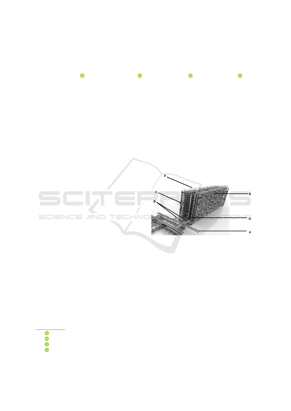
SBS/RS are build with several storage aisles and

levels, see Figure 1. On each ﬂoor, a tier-captive shut-

tle operates. These shuttles handle storage totes and

carry them horizontally from and to the lifts. Each

lift, positioned a the begin of the shelf, is responsible

to carry storage totes vertically from each level to the

I/O point of the SBS/RS. The I/O point being the in-

terface between the SBS/RS and the rest of the ware-

house conveyor system. This allow the totes stored in

the SBS/RS to reach pick station located elsewhere in

the warehouse.

https://orcid.org/0000-0002-7512-8178

https://orcid.org/0000-0001-9183-0365

https://orcid.org/0000-0001-5772-282X

https://orcid.org/0000-0002-0816-0645

Figure 1: Drawing of an SBS/RS with input and output con-

veyor. (A) Warehouse conveyor; (B) Input and Output (I/O)

conveyor section; (C) Lift moving vertically; (D) Racking

level with shuttles moving horizontally; (E) storage loca-

tion; (F) Aisle.

On goods-to-man automated warehouses, human

operators are static at picking stations where the ar-

ticles to pick are bring to them inside storage totes.

Those totes are convoyed from storage locations to

pick station on mechanised conveyors. SBS/RS are

devices holding thousand of storage totes. Upon

request from the Warehouse Management Software

(WMS) they release storage totes holding the stock

to fulﬁll picking orders. The time need to travel from

a storage location to a picking station is the retrieval

time.

In our study, we aim to maximize picking efﬁ-

ciency in automated warehouse by reducing the re-

trieval time of storage totes. We limit the scope of our

study to the SBS/RS, we propose a method to opti-

1040

Courtin, P., Fasquel, J.-B., Lhommeau, M. and Grimault, A.

A Deep Learning Approach to Minimize Retrieval Time in Shuttle-Based Storage Systems.

DOI: 10.5220/0013255300003890

Paper published under CC license (CC BY-NC-ND 4.0)

In Proceedings of the 17th International Conference on Agents and Artiﬁcial Intelligence (ICAART 2025) - Volume 3, pages 1040-1047

ISBN: 978-989-758-737-5; ISSN: 2184-433X

mize the allocation of storage totes (therefore articles)

to storage locations within the SBS/RS. We expect to

minimize the retrieval time by reducing the travel time

(or distance) traveled by shuttles to fulﬁll pick orders.

This problem of selecting the best assignment for ar-

ticles in a warehouse, while minimizing (or maximiz-

ing) objectives functions, is known as the Storage Lo-

cation Assignment Problem (SLAP). We consider ar-

ticles with only one pack size of 1 piece, therefore in

the remainder of this paper articles are identiﬁed as

Stock Keeping Units (SKUs).

The main originality and contribution of this pa-

per is a deep learning-based method using LSTM

to address the Storage Location Assignment Prob-

lem (SLAP) in a Shuttle-Based Storage and Retrieval

System (SBS/RS) warehouse. Our method aims to

tackle peaks situations (sudden and high variation in

requested pieces) occurring for some SKUs identiﬁed

in class Z in the XYZ-Analysis. Another part of the

contribution regards preliminary experiment on a real

dataset.

The remainder of the paper is organize as follow.

In section 2, we present a comprehensive state of the

art on SLAP, covering previous approaches such as

dynamic programming, integer linear programming,

heuristics, and machine learning models like cluster-

ing and deep reinforcement learning applied to logis-

tics. In section 3, we detail our approach which com-

bines Long Short-Term Memory (LSTM) (Hochreiter

and Schmidhuber, 1997) model to predict future de-

mands with an optimization process to assign to stor-

age locations, aiming to minimize shuttle travel time

for articles retrieval. The experiments, detailed in

section 4, compare the performance of this method

against other standard strategies (mean, random, and

naive methods) by evaluating metrics such as bad al-

location rate and retrieval time during peak demand.

The results show that the LSTM model outperforms

the comparative methods by reducing retrieval time,

and it proves particularly effective in handling peak

demand. Finally,in section 5 we discuss future direc-

tions for improving the model, notably enhancing its

scalability to handle larger datasets without relying on

a reference allocation.

2 RELATED WORKS

The SLAP was formalized (Hausman et al., 1976) and

later proved NP-hard (Frazelle, 1989). Several solu-

tions have been proposed to solve the SLAP, such as

exact methods: dynamic programming, integer mixed

linear programming (Reyes et al., 2019), approximate

methods: heuristics (Zhang et al., 2019) and meta-

heuristics (Talbi, 2016) and simulations. Dedicated

storage strategies and policies are also utilize. The

most common strategies are Class-Based (CB): where

SKUs are group into classes depending on various cri-

terion such as ABC-Analysis (Hausman et al., 1976)

or XYZ-Analysis (Nowoty

nska, 2013; Stojanovi

c and

Regodi

c, 2017).

Some studies are addressing the SLAP with ma-

chine learning utilizing k-means Clustering algorithm

(Huynh et al., 2024). Others are introducing explain-

able machine learning models for decision making

based on decision trees (Berns et al., 2021). Another

uses a recurrent network to predict the duration of stay

of pallets in the AVS/RS in order to optimize ware-

house storage assignment (Li et al., 2019).

Other studies, not speciﬁc to logistic, have demon-

strate the capabilities of machine learning algorithm

like Random Forest, K-Nearest Neighbors (K-NN) to

address other allocation problem (Al-Fraihat et al.,

2024).

A recent study solves the SLAP using Reinforce-

ment Learning (Troch et al., 2023). In this study, the

SLAP is solve as a sequential decision-making prob-

lem. A standard Markov Decision Process (MDP)

model is created. The agent aims to optimize the lay-

out by adjusting product locations based on popular-

ity. The reward is calculated using a metric, which

takes into account the number of times products ap-

pear in orders and their distances from pickers. The

solution is then compare with a genetic algorithm ap-

proach.

Another study uses Deep Reinforcement Learning

(DRL) to address dynamic storage location assign-

ment problem (DSLAP) (Waubert de Puiseau et al.,

2022). DSLAP is deﬁned as the problem of determin-

ing where to optimally store goods in a warehouse

upon entry or reentry. (Waubert de Puiseau et al.,

2022) are using Q-Learning with Proximal Policy Op-

timization (PPO) algorithm. Their Objective is to de-

crease transportation costs within the warehouse by

assign pallet to zones (A, B, or C) to locations. The re-

ward is set proportional to each operation’s cost. They

compare results with rule-based benchmark methods

on the test data.

To the best of the authors knowledge, no study ad-

dresses the SLAP using deep learning method (Zarin-

chang et al., 2023). We propose a deep learning model

to dynamical allocate SKUs into storage locations of

a SBS/RS device operating in an automated goods-

to-man warehouse, in order to minimize the retrieval

time of storage totes.

A Deep Learning Approach to Minimize Retrieval Time in Shuttle-Based Storage Systems

1041

3 PROPOSED APPROACH

The proposed method consist of a deep learning algo-

rithm trained with data generated by an optimization

process, based on the following assumptions:

1. We consider only one pack size for articles.

Therefore for the remainder of the paper one ar-

ticle = one Stock Keeping Unit (SKU);

2. Each storage tote is conﬁgured in 1/1. So one and

only one SKU type can be stored in a storage tote;

3. Only one SKU piece is store into a tote;

4. A SKU can be assign to one or more storage tote;

5. SBS/RS is conﬁgured in single deep. Only one

storage tote per storage location;

6. No short picks during picking. Their is enough

stock to fulﬁll picking orders;

7. Replenishment and re-allocation of storage tote

are performed overnight, between shifts.

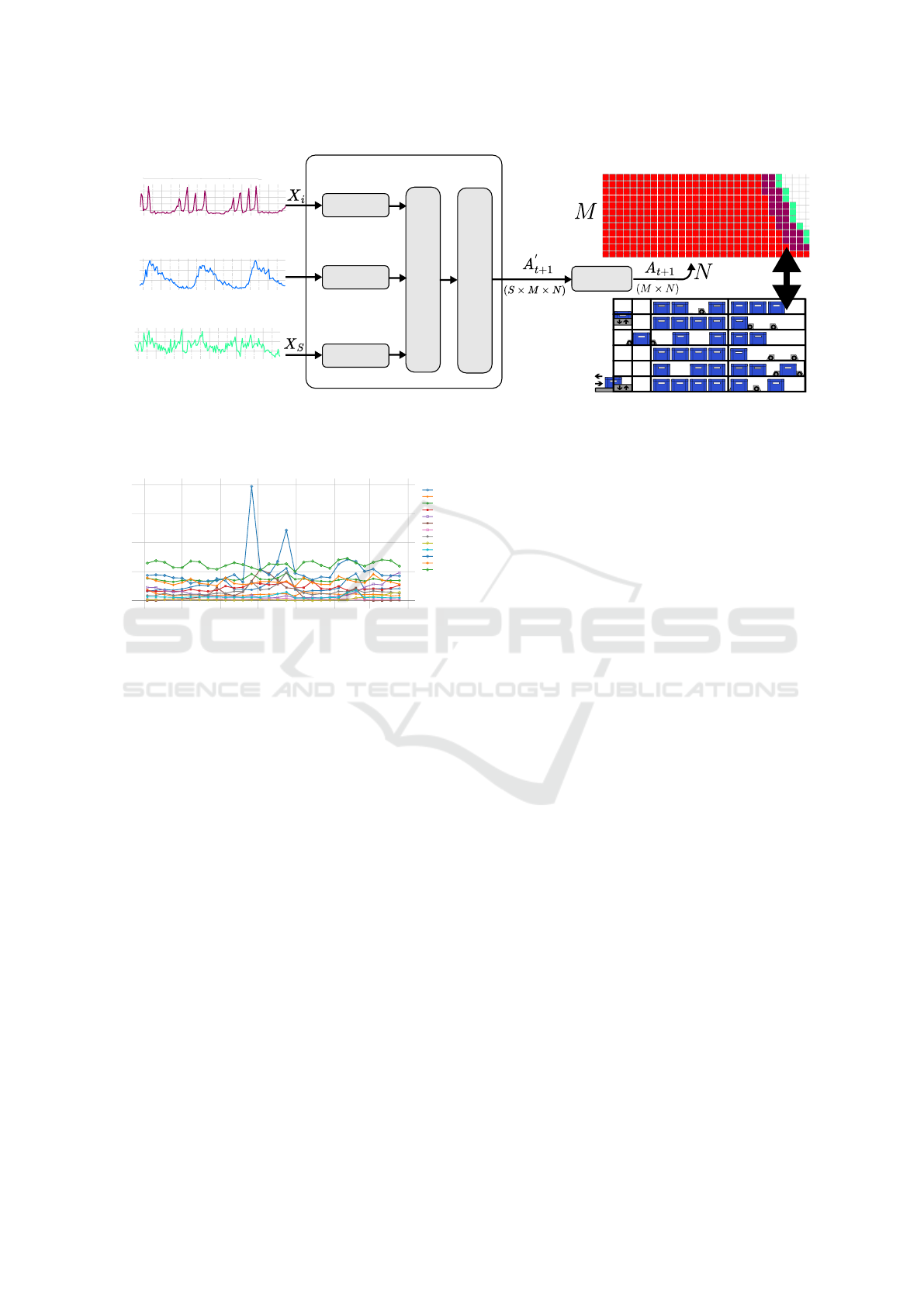
Figure 2 shows an overview of the proposed deep

learning model. Historical data, X

(t) is the number of

requested pieces i ∈ S products at day t, from a past

period (from t − τ to t) are provided to this model,

where S is the set of SKUs. The model provides an

output allocation matrix, A

t+1

, for the next day t + 1.

This allocation matrix A

t+1

(k, l) = i is of size M × N,

with index k ∈ M the height of the SBS/RS (number of

levels) and l ∈ N is the width of the SBS/RS (number

of channels).

In our architecture, a dedicated part handles his-

torical time series data. In this part, for each SKU,

past period ([t − τ;t]) data are processed by an LSTM

(Long Short-Term Memory) network (Hochreiter and

Schmidhuber, 1997). Each LSTM deliver a tensor of

size (τ × lstm hidden size). The LSTM results are

then concatenated and passed to a linear layer. This

layer adds an extra SKU representing empty locations

assignment. The convolution layer subsequently re-

duces the output sequence length (kept by LSTM) to

the model prediction horizon set to (h = 1) for a next-

day prediction (t + 1). Eventually the output of the

model A

′

(t+1)

is a tensor of size (S × M × N). It holds

for each SKU (plus empty locations) the probability

of being assigned to each storage position.

The ﬁnal assignment matrix A

(t+1)

, of size (M ×

N), is computed using the argmax function:

(t+1)

(k, l) = argmax

′

(t+1)

(s, k, l),

which selects the index of the SKU with the highest

probability for each storage location (k, l).

The model is trained using optimal assignment

matrices, together with related inputs. Optimal matri-

ces are produced using a mixed integer programming

model which solves the SLAP ((Kellerer et al., 2004),

(Zhang et al., 2019)). The solution of this optimiza-

tion model is referred as the ground truth thereafter.

The optimization criterion is to minimize the cost

of retrieving SKUs considering the binary decision

variable x

s,k,l

equal to 1 if the SKU s ∈ S is assigned

to the position k ∈ M, l ∈ N. In such case, the cor-

responding allocation index A

t+1

(k, l) = s is directly

linked to the value of variable x

s,k,l

For each each storage location (k, l) the cost of

retrieving a SKUs from a storage location to the I/O

entry/exit point of the SBS/RS, is noted c

k,l

. The re-

trieval cost is computed using velocity and accelera-

tion of shuttles and lifts.

The objective function to be optimized can be for-

mulated as follow in Equation 1.

z = min

∑

s∈S

∑

k∈M

∑

l∈N

s,k,l

· c

k,l

(1)

∑

s∈S

s,k,l

≤ 1 ∀k ∈ M∀l ∈ N (2)

∑

k∈M

∑

l∈N

s,k,l

= 1 ∀s ∈ S (3)

s,k,l

∈ {0, 1} ∀s ∈ S, ∀k ∈ M, ∀l ∈ N

Constraint (Equation 2) imposes only one SKU

for each position, constraints (Equation 3) imposes

only one position for each SKU. These constraints

could be extended based on other properties associ-

ated with SKUs, such as the problem of compatibility

between products (i.e. perishable or ﬂammable prod-

ucts).

4 EXPERIMENTS AND RESULTS

In this section, ﬁrst we outline the dataset used and the

conﬁguration of the model. Then we introduce the

evaluation metrics and ﬁnally we present the results

over a real dataset.

4.1 Dataset

The input data represents the daily demand of pieces

to pick for a set of SKUs in an automated warehouse.

Those timeline have been extracted from a publicly

available data ”Retail Data Analytics” hosted on Kag-

gle

. This dataset holds historical weekly sales data

from 45 stores, over a period from May 2010 to Jan-

uary 2012 (143 weeks).

https://www.kaggle.com/datasets/manjeetsingh/

retaildataset?select=sales+data-set.csv

ICAART 2025 - 17th International Conference on Agents and Artiﬁcial Intelligence

1042

I/O

point

LSTM

Linear

Conv1D

AllocationNet

# pieces requested

Allocation matrix

timestamp

LSTM

......

argmax

Jul 2010 Jan 2011 Jul 2011 Jan 2012 Jul 2012

Figure 2: Overview of the proposed approach, using historical data, the model will allocate SKUs to storage locations.

(right) Historical data, pieces requested per SKU. (middle) Our deep learning model. (left) Produced allocation matrix and a

representation of the SBS/RS side view.

Sep 2010 Oct 2010 Nov 2010 Dec 2010 Jan 2011 Feb 2011 Mar 2011 Apr 2011

100

150

200

SKUs

Dataset Overview

date

# pieces requested

Figure 3: Dataset overview of a subset (30 days) of the time

series of number of pieces requested for 13 SKUs for 143

days (local view of superimposed data, compared to Figure

2). For example, SKU M (+) as a seasonal behavior, SKU

K (⋄) as peaks in November 2010 and December 2010.

Each original store is composed with up to 100

department. As we consider only one warehouse in

our study, for each 45 stores we merge (sum up) the

weekly sales for each department. From 100 avail-

able departments, we keep a subset of 13 departments

and considered each department as a unique SKU. We

also consider each weekly sale entry as a day entry.

The selection was made to keep timelines with

even demand (class X from XYZ-Analysis), sea-

sonal behaviour (class Y from XYZ-Analysis) and

timelines with peaks (class Z from XYZ-Analysis).

We keep following departments: 1, 3, 4, 11, 16,

18, 35, 55, 56, 67, 72, 79 and 91. Figure 3

presents an overview of the dataset used. For all

SKUs, in average 300 pieces are requested every day.

The minimal and maximal daily request 233 and 483.

The minimum and maximum number of pieces to per

SKU are respectively 0 pieces for SKU F and I and

203 pieces for SKU K.

4.2 Model Conﬁguration

We implemented and conducted the experiments us-

ing Python 3.12.0 and implemented the deep learn-

ing model with PyTorch 2.3.1 package. Ground

truth allocation matrices for training purposes have

been generated with a MIP model implemented and

solved with OR-Tools 9.8.3. We trained our model

using supervised training method. The model was

conﬁgured with the following hyper-parameters: τ =

8, N = 40, M = 15 and S = {1, . . . , 13}. The number

of hidden units per LSTM layer is set to 600. This

lead to a model with # 84,342,009 trainable param-

eters.

Training was computed over 1000 epochs, using

Mean Squared Error (MSE) as the loss function. We

used Adamax algorithm for the gradient descent, with

learning rate γ = 0.002, betas β

= 0.9, β

= 0.999

and epsilon ε = 1e

−08

. We used a reduce learning rate

technique with a patience of 10 epochs, factor 0.1 in

minimizing mode. No data pre-processing was per-

formed (i.e. no scaling, normalization nor standard-

ization of the data)

Dataset have been split into training, validation

and testing sets, 50%(71 days), 10% (14 days) and

40% (57 days) of the whole dataset. Due to the lim-

ited size of dataset (143 days) and the training subset

(71 days), we expanded the training data by repeating

it 10 times to accelerate the training process. As a re-

sult, during each training epoch, our model effectively

trains on a dataset equivalent to 710 days instead of

the original 71 days.

A Deep Learning Approach to Minimize Retrieval Time in Shuttle-Based Storage Systems

1043

Nov 2010 Jan 2011Dec 2010 Feb 2011

100

150

200

Pieces requested per SKU

period

# pieces requested

Allocation at t=46

Figure 4: Ground truth dataset overview, input, and output data. (left) Number of pieces requested for each 13 SKUs for 16

days displayed (right) Allocation of SKUs into the 600 storage locations for timestamp t = 46.

4.3 Allocation Methods for Comparison

Purposes

To assess the efﬁciency of our proposed pipeline, we

compare it’s allocations against three other standard

methods, as well as with the ground truth. As detail in

previous paper (Courtin et al., 2024), we will compare

with Mean, Naive and Random methods. All methods

will return an allocation of SKUs for the next day t +

• Mean: method consists of determining the num-

ber of pieces request for each SKU at t + 1 then

assign SKUs. It computes the average demand

over the last 30 days (as usually performed in the

industry). Then SKUs are assigned to location

based on their demand. Highly demanded SKUs

are stored into free storage locations with cheap-

est retrieval cost;

• Naive: method is based data from the previous

day. The number of pieces request for each SKU

at t + 1 is considered the same as current day

t. Then the SKUs are assigned like describe in

method Mean;

• Random: method randomly assigns SKUs to

storage locations following a uniform distribution.

The number of pieces per SKUs at t +1 is not cal-

culated but known from input data.

4.4 Evaluation Metrics

To compare allocations between methods, we intro-

duce the following metrics: Bad Allocation Rate, Re-

trieval Time and Retrieval Time on Peaks:

• Bad Allocation Rate. (BAR), expressed in per-

centage, measures the difference of the number of

storage locations used by a method and their po-

sitions compared to the ground truth. A low BAR

value, close to 0%, means that the allocation of the

method is close from the ground truth. It indicates

a small variation in numbers and positions of the

selected storage locations. Higher BAR scores,

closer to 100%, are implying to much (or to few)

storage locations used and a spread of the selec-

tion.

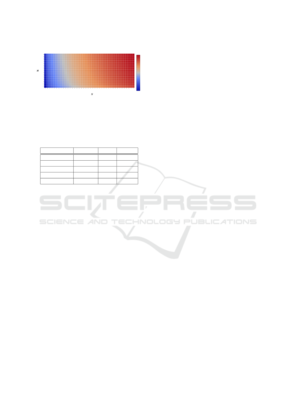
• Retrieval Time. (RT) measures the number of

seconds required to take-out all requested SKUs

from the SBS/RS. Retrieval time is computed us-

ing the retrieval cost of each storage location and

the number of pieces to pick per SKU, see. The

retrieval cost is calculated using shuttles and lifts

velocity and acceleration Figure 5. We also intro-

duce a penalty to retrieval times. If a method does

assigned enough storage locations to fulﬁll daily

request, extra storage location are assigned and a

penalty is added to the RT. The penalty is equals to

storage location retrieval cost double. This aims

to simulate the additional time required to replen-

ish the SBS/RS with the missing pieces.

• Retrieval Time for Peaks. (RTP) measures the re-

trieval time of SKUs only at peaks timestamps.

This metric allows us to assess if a method is

able to detect and react to peaks in SKUs de-

mands (handling the case of class Z in the XYZ-

Analysis).

4.5 Results

Table 1 presents the compiled results of metrics com-

puted from the allocations provided by all methods

on the real dataset. It presents the daily average value

of each metric: BAR, RT with penalty, and the RTP

timestamps for each allocation method.

We observe that our approach provides the best

score for each metric. For the BAR, the small score of

our method indicates than the positions and number of

selected storage locations are close from the ground

truth. The small RT and RTP indicate that our method

ICAART 2025 - 17th International Conference on Agents and Artiﬁcial Intelligence

1044

0 1 2 3 4 5 6 7 8 9 10 11 12 13 14 15 16 17 18 19 20 21 22 23 24 25 26 27 28 29 30 31 32 33 34 35 36 37 3839

retrieval

time [s]

Cost matrix

Figure 5: Cost Matrix example. For each storage location

time in seconds need to retrieve a SKU from the location to

the I/O point. I/O points set at level 0 and channel 0. Stor-

age locations closer to this point have the smallest retrieval

time.

Table 1: Metrics compiled results on real dataset for 13

SKUs. Daily average value of Bad Allocation Rate (BAR),

Retrieval Time (RT) and Retrieval time on peaks (RTP) for

each allocation method.

Method BAR [%] RT [s] RTP [s]

Random 48.96 3425 3526

Mean 21.35 3763 4704

Naive 5.57 2935 3736

Our approach 3.20 2917 3367

Ground truth – 2525 3154

(event with penalties) provides ”goods” allocations to

keep the retrieval time low. SKUs are correctly sorted

and put to the I/O point depending of the demand.

The Random allocation strategy gives a mean

BAR of 48.96%, meaning almost half of the selected

location by this methods are different one than the lo-

cations selected in ground truth. The Mean method

yields a BAR of 21.35%, implying a bad selection

of storage location almost every ﬁfth allocation. The

Naive method provides a BAR of 5.57%. Our method

returns the smallest BAR of 3.2 %, meaning our deep

learning model, for the same input data, will selected

the same storage locations than the one selected by

ground truth 96 % of the time. An example of differ-

ence in locations selection is illustrated in Figure 7.

Concerning retrieval time, Mean method provides

the highest retrieval time with 3763 seconds in aver-

age. The Random method provides better than Mean

with a RT of 3425 seconds. Naive and our method

provide the smallest retrieval time with respectively

2935 and 2917 seconds.

Regarding retrieval time at peaks timestamp, the

Mean method yields the longest retrieval time, 4704

seconds. This may be explained by the missing lo-

cations selected, because of the wrong assumption of

number of pieces to pick calculated by average mean

of 30 days. Then Naive method gives a RT of 3736

seconds on peaks timestamp. Random method per-

form again surprisingly well, with the second best RT

on peaks of 3526 seconds. This may be explained by

the absence of penalty applied to this method. For

this method storage location are choose randomly but

the number of pieces to pick at t + 1 is known from

the historical data (like ground truth). Eventually our

method allows for the smallest RT on peaks with 3367

seconds.

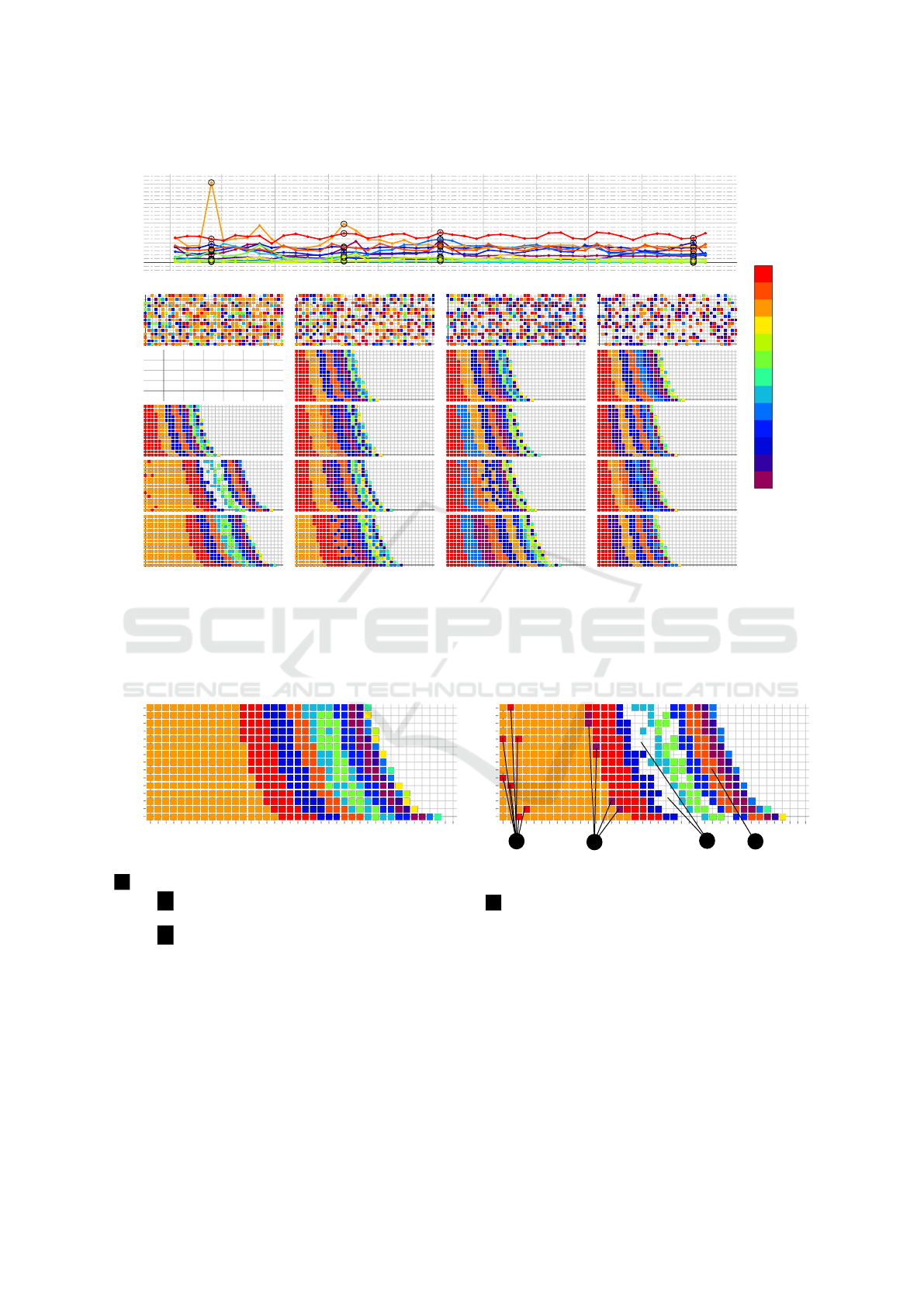
Figure 6 displays examples of allocations pro-

vided provided by each method and ground truth at

4 timestamp. One timestamp t = 13 during a peak

of SKU K it’s demand varies starts from 43 pieces,

reach peak of 200 pieces and drops to 55 pieces re-

quested. Only our method is able to identify the peak.

Another timestamp t = 24 displays allocation for a

smaller peak of SKU K. In this situation our method

as swapped the most requested SKU K with the sec-

ond most requested E with respectively 98 and 74

pieces to pick. Another timestamp t = 32 a usual daily

demand with signiﬁcant raise in demand of SKU E.

Here our method react correctly for the second most

requested SKU E (59 pieces), but the third SKU A

(57 pieces) was put behind other SKUs, this will lead

to high penalty retrieval time. Eventually timestamp

t = 53 where SKU B becomes the second most re-

quested SKU. Note: Because of the size of the test

dataset, the position of the signiﬁcant peak in demand

for product K and the 30 days need to compute the al-

location, the Mean method cannot provide allocations

for the ﬁrst displayed timestamp.

This ﬁgure illustrates the ability of our method

to handle signiﬁcant peaks in SKU demand, like at

timestamp t = 13. But some locations in the middle

of the SBS/RS are left empty, see Figure 7. And some

assignments are swapped compared to ground truth.

This indicates that our Model could be further trained.

Despite those swapped, misplaced or empty alloca-

tions our method provides the best BAR, RT and RTP

scores.

Experiments conducted on a real dataset have

demonstrated that our deep learning model using

LSTM was able to allocated SKU to storage location

with decent performances. The low BAR scored in-

dicates that allocations provided where close to the

ground truth (in number and positions). The small

RT value on peaks indicates the ability to handle

peaks situations. Regarding RT for the whole period

our method return the lowest score. Although naive

method returns the second best score on BAR and RT

metrics.

A Deep Learning Approach to Minimize Retrieval Time in Shuttle-Based Storage Systems

1045

Nov 2011 Jan 2012 Mar 2012 May 2012 Jul 2012 Sep 2012

100

150

200

Sku name

Allocations comparison on real dataset

# pieces requested

randommeannaivelstm

ground_truth

Allocation at t=13 Allocation at t=24 Allocation at t=32 Allocation at t=53

Figure 6: Methods allocations comparison. (top) Timeline of number of requested pieces for each SKU over 45 days. (bottom)

Allocations provided by each method and ground truth for 4 timestamp. One timestamp t = 13 during a peak of SKU K.

Another timestamp t = 24 displays allocation for a smaller peak of SKU K. Another timestamp t = 32 a usual daily demand

with signiﬁcant raise in demand of SKU E. Eventually timestamp t = 53 where SKU B becomes the second most requested

SKU. Note: Because of the size of the test dataset, the position of the signiﬁcant peak in demand for product K and the 30

days need to compute the allocation, the mean method cannot provide allocations for the ﬁrst displayed timestamp.

0 5 10 15 20 25 30 35 39

Ground Truth

channel

level

channel

Prediction LSTM

Figure 7: Example of allocations at peak timestamp provided by ground truth (left) compare to our method (right). At marker

a between channel 0 and 5, we observe misplace allocations of SKU M, it should not be place so close from the I/O. At

marker b SKU A has 5 misplaced reserved locations. At marker c between channels 20 and 25 some locations have been

left empty. This means shuttles need to cross this empty section for retrieving operations, impacting the retrieval time. At

marker d SKU L have been assigned farther from the I/O point They should have been place after the SKU H in the empty

space. All those misplacement, swap and empty space contribute to downgrade the RT score of our method. This indicates

that our Model could be further trained.

5 CONCLUSION AND

PERSPECTIVES

We have proposed a new data-driven approach to

address the Storage Location Assignment Problem

(SLAP) with a deep learning model using LSTM. Our

proposed method generates assignments of SKUs in

SBS/RS storage locations based on historical picking

orders. On a previous work we utilize our model on

a synthetic generated dataset. The follow-up experi-

ments conducted in this paper on a real dataset have

ICAART 2025 - 17th International Conference on Agents and Artiﬁcial Intelligence

1046

shown that our model, reduces shuttles retrieval time,

is capable to process real data and able to handle peak

situations.

Our deep learning model outperformed other

methods and provides a lower BAR and smaller re-

trieval time.

A limitation of our proposal is the requirement of

generating ground truth allocations for training, there-

fore requiring mixed integer programming techniques

that could be time consuming.

An alternative to study is to design a loss func-

tion based on the retrieval time of predicted alloca-

tions, instead of using a loss which compares pre-

dicted and ground truth allocations. We aim at train-

ing our model without generating ground truth data

(allocations for the next day) beforehand. For future

work, we will design a loss that will assess the error

(or ”correctness”) of the allocations returned by our

Deep Learning model and allow us to perform back-

propagation based on this error and adjust our model

weights accordingly. This custom loss will compute

an error score using the SBS/RS cost matrix, pre-

dicted SKUs allocations probability and the number

of pieces to pick.

ACKNOWLEDGEMENTS

Funding: All research in this study was funded by

KNAPP France. There was no external funding.

Competing interests: This work was done in the

course of employment at KNAPP France, with no

other competing ﬁnancial interests. Data and mate-

rials availability: This work used publicly available

data from Kaggle

REFERENCES

Al-Fraihat, D., Sharrab, Y., Al-Ghuwairi, A.-R., Alzabut,

H., Beshara, M., and Algarni, A. (2024). Utiliz-

ing machine learning algorithms for task allocation

in distributed agile software development. Heliyon,

10(21):e39926.

Berns, F., Ramsdorf, T., and Beecks, C. (2021). Machine

Learning for Storage Location Prediction in Indus-

trial High Bay Warehouses, page 650–661. Springer

International Publishing.

Courtin, P., Grimault, A., Lhommeau, M., and Fasquel, J.-

B. (2024). A deep learning approach to address the

storage location assignment problem. ICAART 2024,

Doctoral Consortium.

Frazelle, E. H. (1989). Stock location assignment and order

picking productivity. PhD thesis, Georgia Institute of

Technology.

Hausman, W., Schwarz, L., and Graves, S. (1976). Optimal

Storage Assignment in Automatic Warehousing Sys-

tems. Management Science, 22(6).

Hochreiter, S. and Schmidhuber, J. (1997). Long short-term

memory. Neural Computation, 9(8):1735–1780.

Huynh, H.-D., Nguyen, D. D., Do, N.-H., and Nguyen,

K.-V. (2024). A Clustering Algorithm for Storage

Location Assignment Problems in E-commerce Ware-

houses, page 251–265. Springer Nature Switzerland.

Kellerer, H., Pferschy, U., and Pisinger, D. (2004). Knap-

sack Problems. Springer, Berlin, Germany.

Li, M. L., Wolf, E., and Wintz, D. (2019). Duration-of-stay

storage assignment under uncertainty.

Nowoty

nska, I. (2013). An application of XYZ analysis

in company stock management. Modern Management

Review.

Reyes, J. J. R., Solano-Charris, E. L., and Montoya-Torres,

J. R. (2019). The storage location assignment prob-

lem: A literature review. International Journal of In-

dustrial Engineering Computations, page 199–224.

Stojanovi

c, M. and Regodi

c, D. (2017). The signiﬁcance

of the integrated multicriteria ABC-XYZ method for

the inventory management process. Acta Polytechnica

Hungarica, 14(5):20.

Talbi, E.-G. (2016). Combining metaheuristics with math-

ematical programming, constraint programming and

machine learning. Annals of Operations Research,

240(1):171–215.

Troch, A., Mannens, E., and Mercelis, S. (2023). Solving

the storage location assignment problem using rein-

forcement learning. In Proceedings of the 2023 8th

International Conference on Mathematics and Artiﬁ-

cial Intelligence, ICMAI 2023, page 89–95. ACM.

Waubert de Puiseau, C., Nanfack, D., Tercan, H., L

obbert-

Plattfaut, J., and Meisen, T. (2022). Dynamic storage

location assignment in warehouses using deep rein-

forcement learning. Technologies, 10(6):129.

Zarinchang, A., Lee, K., Avazpour, I., Yang, J., Zhang, D.,

and Knopf, G. K. (2023). Adaptive warehouse stor-

age location assignment with considerations to order-

picking efﬁciency and worker safety. Journal of In-

dustrial and Production Engineering, 0(0):1–20.

Zhang, R.-Q., Wang, M., and Pan, X. (2019). New model of

the storage location assignment problem considering

demand correlation pattern. Computers & Industrial

Engineering, 129:210–219.

A Deep Learning Approach to Minimize Retrieval Time in Shuttle-Based Storage Systems

1047