Deep Learning-Based Vessel Traffic Prediction Using Historical Density
and Wave Features
Dogan Altan
1 a
, Dusica Marijan
1
and Tetyana Kholodna
2
1
Simula Research Laboratory, Oslo, Norway
2
Navtor AS, Egersund, Norway
Keywords:
Vessel Traffic Prediction, Automatic Identification System, Historical Density, Wave Features, Tailored
Features.
Abstract:
Sea traffic is fundamental information that needs to be considered while planning vessel operations to enhance
navigational safety and operational efficiency. Therefore, several environmental constraints, such as weather
and traffic conditions, must be taken into account to minimize delays caused by vessel traffic and improve
safety by decreasing collision risks. In this paper, we address the vessel traffic prediction problem, which
tackles predicting vessel traffic for ships using several sources of information. We propose a vessel traffic
prediction method that processes information obtained from different sources indicating historical traffic and
wave conditions for vessels. The proposed method consists of three models processing different types of fea-
tures and fuses the outputs of these models for the vessel traffic prediction problem. We evaluate the proposed
method on real-world historical vessel trajectories and report its performance by providing a comparison with
other baselines. The experimental results indicate that our proposed method provides promising results for
predicting vessel traffic with a mean squared error of 0.325.
1 INTRODUCTION
Due to the immense growth in the share of maritime
transportation in the global economy, vessel traffic
at sea has significantly increased (Wan et al., 2016).
Such an increase necessitates considering vessel traf-
fic while planning maritime operations to improve op-
erational efficiency (Teng et al., 2017). As heavy ves-
sel traffic might lead to delays in the estimated time of
arrival (ETA) of ships to their destination ports (Bo-
dunov et al., 2018), it is essential to take into account
traffic density to minimize delays. In this paper, we
address the vessel traffic prediction problem, which
deals with estimating the number of vessels that will
sail in certain areas in a future time step.
Vessels broadcast automatic identification system
(AIS) messages, which include information related to
the vessel and voyage for identification and tracking
purposes. Generally, an AIS message includes several
features, including timestamp, speed over ground,
course over ground, and heading. In most cases, while
broadcasting such messages, the vessels sail through
a set of planned locations named waypoints. Such
a
https://orcid.org/0000-0002-5053-4954
waypoints, along with other voyage-related informa-
tion (i.e., planned speed), form passage plans. Way-
points are generally defined considering the locations
where vessels change their behavior significantly (i.e.,
direction, speed, etc.).
Maritime traffic prediction is vital for safety and
voyage optimization, and it contributes to situational
awareness (Xiao et al., 2019). The traffic prediction
problem can be tackled from several perspectives us-
ing linear or non-linear methods from either trajec-
tory or location level (Xiao et al., 2019). Trajectory
level solutions generally rely on predicting future ves-
sel positions (which is known as the trajectory predic-
tion problem (Zhang et al., 2022)) and constructing a
density map accordingly from the predicted trajecto-
ries. Such trajectory prediction techniques rely highly
on AIS quality and are restricted in how far (i.e., the
number of hours) they can accurately forecast in the
future. Consequently, these limitations might pose
constraints on how far in advance the expected traf-
fic can be estimated for safe navigation. Another ap-
proach would be to represent the locations of inter-
est particularly (i.e., such as grids or graphs) and then
predict the heavy traffic areas (i.e., hotspots), which
are locations with a higher number of vessels. On
1054
Altan, D., Marijan, D. and Kholodna, T.
Deep Learning-Based Vessel Traffic Prediction Using Historical Density and Wave Features.
DOI: 10.5220/0013258100003890
Paper published under CC license (CC BY-NC-ND 4.0)
In Proceedings of the 17th International Conference on Agents and Artificial Intelligence (ICAART 2025) - Volume 3, pages 1054-1061
ISBN: 978-989-758-737-5; ISSN: 2184-433X
Proceedings Copyright © 2025 by SCITEPRESS – Science and Technology Publications, Lda.

the other hand, such techniques generally handle the
problem from a location perspective, where represen-
tations, such as grid representations, are used for a re-
gion of interest, leading to challenges related to scal-
ability issues for global solutions.
As sea conditions are external factors essential for
safe navigation (Perera and Soares, 2017; Zis et al.,
2020), it is crucial to incorporate information related
to sea conditions to predict vessel traffic to enhance
the efficiency and safety of vessel operations. Fur-
thermore, vessel traffic prediction can help avoid con-
gested areas at sea (i.e., canals) or ports, decreasing
the risk of delays and collisions. In this paper, we
handle the vessel traffic prediction problem from a
trajectory-level aspect in an offline manner where ex-
pected instant traffic around a vessel is predicted for
each AIS message, taking into account historical den-
sity features, tailored features (i.e., features obtained
by processing AIS messages and passage plans), and
wave-based features. Such an offline approach en-
ables the prediction of vessel traffic earlier, only de-
pending on the availability of predictions of sea con-
ditions (i.e., waves), unlike the existing approaches
where the vast majority focuses on regional solutions
for solving the maritime traffic prediction problem
with a limit on how far in the future the predictions
can be made. The contributions of this study are as
follows:
• We handle the maritime traffic prediction problem
from a global trajectory-level perspective with-
out explicitly predicting the future locations of the
vessel or using a region-based perspective.
• We take into account three different types of fea-
tures: historical density, wave, and tailored AIS
features (obtained from both AIS messages and
passage plans). We process these features within
distinct, specific models and fuse the outputs of
these models to predict the vessel traffic.
• We evaluate the proposed traffic prediction on
real-world AIS data, provide a comparative anal-
ysis with baselines, and also provide an ablation
analysis in which the contribution of each distinct
model employed in the proposed method is ana-
lyzed.
The paper is organized as follows: First, we sum-
marize the literature on the maritime traffic prediction
problem. Then, we elaborate on our proposed traffic
prediction method. Later, we present the evaluation
of the method. Finally, we conclude the paper with
potential future directions.
2 RELATED WORK
Classical machine learning methods are widely stud-
ied in the literature for addressing the maritime traffic
prediction problem. Kalman filters are employed in
one study to predict vessel traffic flow between the
Wuhan Yangtze River Bridge and the Second Wuhan
Yangtze River Bridge (Wei et al., 2017). Another
method addresses the maritime traffic density predic-
tion problem (Rong et al., 2022) by extracting ship
motion prediction models and maritime traffic graphs.
The maritime graphs are extracted using the Ordering
Points To Identify the Clustering Structure (OPTICS)
algorithm. Logistic regression is used to model the
destination of ships, and Gaussian processes are used
to model ship motions. Then, future positions are pre-
dicted 60 minutes ahead for the Portugal region.
Deep learning techniques are intensively investi-
gated to address the vessel traffic flow problem. In
one work (Liang et al., 2022), graph convolution is
studied, and a maritime graph consisting of feature
points (i.e., starting/ending points and waypoints) is
extracted through processing AIS-based vessel tra-
jectories. This is followed by constructing spatio-
temporal structure of vessel traffic data. Later, multi-
graph convolution for three different graphs (distance,
interaction, and correlation) takes place to predict ves-
sel traffic flow. In another study (Li et al., 2023),
convolutional neural networks (CNN) are employed
together with long short-term memories (LSTM) to
predict vessel traffic flow. Vessel traffic data is trans-
formed into two-dimensional matrices (hour of the
day and day), and convolution results are fed into
LSTM units. Channel similarity information is also
fed into distinct LSTM units, and then the results
are concatenated with a fully connected layer to pre-
dict vessel traffic flow. Another method employs an
LSTM-based method to first predict vessel trajecto-
ries and then employs transformers to predict traf-
fic flow for given locations, which are represented
as grids, within a time frame of up to 30 minutes
(Mandalis et al., 2024). Yet another deep learning-
based method uses LSTMs with dung beetle opti-
mizer (DBO) to predict vessel traffic flow (Dong
et al., 2024), which is based on only AIS, ignoring
external factors such as waves for traffic forecasts.
In another LSTM-based method, Xie and Liu (2018)
propose a method to address vessel traffic flow pre-
diction problem for inland waterways considering the
water level effect.
Signal processing methods are also investigated
in the literature to address the vessel traffic predic-
tion problem. One study investigates discrete wavelet
decomposition to predict traffic flow in Wuhan Port
Deep Learning-Based Vessel Traffic Prediction Using Historical Density and Wave Features
1055

AIS Messages
Copernicus Data
Historical Density Extraction
Wave Feature Extraction
Tailored Feature Extraction
Density Model
Wave Model
Tailored Feature
Model
Fusion
Model
Traffic
Prediction
Passage Plans
Figure 1: General overview of the presented traffic prediction method.
Yangtze River Bridge (Wang et al., 2021). On the
other hand, such a technique uses only hourly ves-
sel traffic flow data to address the problem, ignoring
other factors such as sea conditions (i.e., waves).
There exist various works incorporating weather
data to predict vessel traffic flow. In one study (Huang
et al., 2024), a vessel traffic knowledge graph (i.e.,
wind speed, air temperature of a river) containing the
relations in the region of interest is incorporated with
the traffic flow and processed within a graph atten-
tion network (GAT) and LSTMs to predict vessel traf-
fic on a specified region. Another study that takes
into account weather information to predict vessel
traffic in the Xiazhimen channel using Gated Recur-
rent Units (GRU) with an attention mechanism (Xiao
et al., 2022).
Vessel traffic on ports has also been investigated in
the literature to improve port operations (Parola et al.,
2021). One work uses fuzzy neural networks (FNN)
optimized by a quantum genetic algorithm to predict
the port density of a port located in China (Su et al.,
2020).
Different from earlier studies, we address the ves-
sel traffic prediction problem from a global trajectory-
level perspective without explicitly predicting future
locations of the vessels or considering a location-
specific method, whereas the primary focus of the ear-
lier work is mainly on location-based perspectives.
We handle the vessel traffic prediction problem by
capturing historical traffic patterns along with wave
conditions at sea for abstracted locations (i.e., using
features such as distance to the free sailing area).
Such a perspective enables the prediction of vessel
traffic for a given trajectory without an explicit loca-
tion representation, such as grids or graphs.
3 PROPOSED METHOD
The proposed method processes three different data
sources as inputs: AIS messages, Copernicus data
and passage plans. Features are extracted from these
sources and processed in separate models to predict
vessel traffic. Figure 1 depicts a general overview of
the proposed method. In this section, we explain the
features taken into account in our traffic prediction
method, followed by the explanation of the designed
deep learning model to predict vessel traffic.
3.1 Processed Features
We consider three types of features: historical traffic
density, wave-related features and tailored features.
The historical density features are obtained from his-
torical AIS messages, wave-related features are ob-
tained from Copernicus
1
, and tailored features are ob-
tained from using both AIS messages and passage
plans. The following subsections elaborate on each
processed feature type.
3.1.1 Historical Traffic Features
In this paper, AIS messages are used to extract the
traffic information (i.e., the number of vessels around
the vessel) related to the location (i.e., latitude and
longitude) where the corresponding AIS messages are
related. To do so, we use the Hierarchical Spatial
Index (H3) index representation provided by Uber
2
.
We take into account intersections of vessel trajecto-
ries, which consist of sequential AIS messages, with
the locations that correspond to the H3 cells. Con-
sequently, the number of interactions within an H3
1
https://www.copernicus.eu/en
2
https://github.com/uber/h3
ICAART 2025 - 17th International Conference on Agents and Artificial Intelligence
1056

cell for a given time period provides the vessel traf-
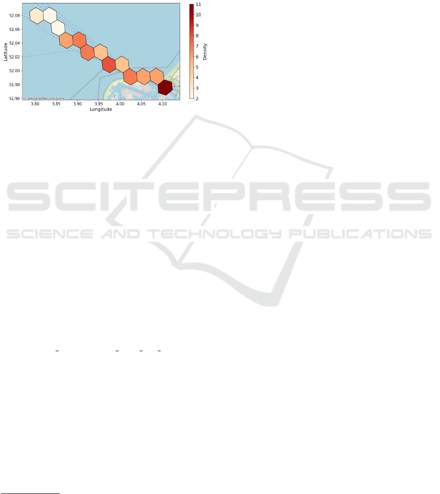
fic for that particular H3 cell. Figure 2 depicts an
example of sequential H3 indices represented with
hexagons for a ship that starts sailing near Rotter-
dam, the Netherlands. Each hexagon corresponds to
an H3 index for given latitude and longitude infor-
mation, and colors represent the traffic density on the
particular hexagons. For clarity, note that the figure
only depicts the initial part of the vessel’s voyage.
Figure 2: Example hexagons corresponding to an H3 index
sequence with the hourly density values for a vessel sailing
from Rotterdam.
We consider historical density features, which are
related to the density (i.e., traffic) of the related loca-
tions in the previous years. In this paper, we take into
account the density information (instant and average)
of the last three years. Instant historical density cor-
responds to the hourly traffic for a given region (i.e.,
H3 index) on the exact day and month of the previous
years. Average historical density corresponds to the
average historical traffic in the related region for the
time span of the trajectory in the prior years (i.e., the
exact start and end day and month of the AIS trajec-
tory but for a previous year).
3.1.2 Wave Features
Historical wave information related to the sea is ob-
tained from Copernicus. The dataset with the product
ID GLOBAL
MULTIYEAR WAV 001 032 is used
to obtain historical wave data
3
. We use the following
features related to wave data from this dataset: spec-
tral significant wave height, spectral significant swell
wave heights of primary and secondary swell, stokes
drift, spectral moments for primary and secondary
swell wave periods, spectral moments wind wave pe-
riod, spectral moments wave period, and wave period
at spectral peak/peak period.
3
https://doi.org/10.48670/moi-00022
3.1.3 Auxiliary Tailored Features
Complementary information is extracted from AIS
messages and passage plans as auxiliary tailored fea-
tures. We use planned speed over ground, distance
to the free sailing area, hour and the completion ra-
tio of the voyage by the ship as tailored features. The
planned speed over ground is obtained from the pas-
sage plan, and this feature is set for each leg (i.e., voy-
age segment between two consecutive waypoints) of
the voyage. The distance to the free-sailing area fea-
ture describes the closest distance of the ship (in nau-
tical miles) to the edge of the free-sailing area. Note
that each free-sailing area is defined as a polygon, and
if the ship sails outside a free-sailing area, its value is
zero. We divide each day into four 6-hour quarters
and use it as the hour feature. The spatial comple-
tion ratio corresponds to the rate at which a ship com-
pletes its voyage. Note that we take into account the
vessel’s location to calculate this feature, instead of
the voyage duration. For instance, when the vessel’s
speed is zero, and it is waiting, this feature’s value
does not change. This feature takes a value between
0 and 1, depending on what the ship’s progress is.
For instance, if the vessel is around the middle of the
voyage, its value is around 0.5, approaching 1 when
the ship approaches the destination port. Note that
the proposed method does not process location fea-
tures (i.e., latitude, longitude, or H3 index) but rather
features associated with the locations (e.g., historical
density, wave and tailored features).
3.2 Traffic Prediction Model
Our proposed traffic prediction method consists of
three models, and in this subsection, we elaborate on
these model structures.
3.2.1 Density Model
The density model (DM) accepts the density features
explained in Section 3.1.1. As consecutive histori-
cal density information forms a sequence, the histor-
ical density is handled temporally in this particular
model. Therefore, we employ an LSTM (Hochreiter,
1997) structure to capture temporal dependencies in
the historical density data, whose number of units is
64. The historical density features are fed into this
model while preserving the yearly chronological or-
der of the density features.
3.2.2 Wave Model
The wave model (WM) accepts the features explained
in Section 3.1.2, and similar to the density model ex-
Deep Learning-Based Vessel Traffic Prediction Using Historical Density and Wave Features
1057

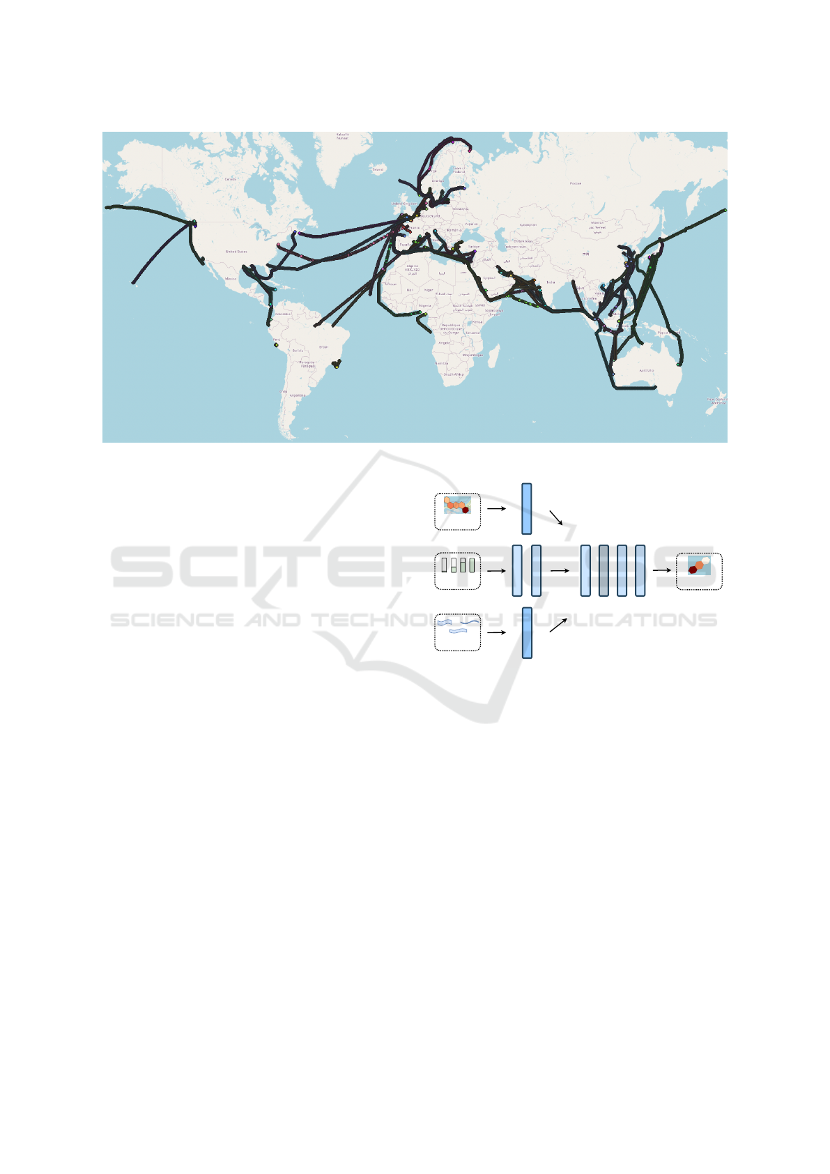
Figure 3: The dataset used in the experiments consists of 263K AIS messages obtained from vessels sailing worldwide.
plained in Section 3.2.1, an LSTM structure is used
to temporally process the historical and current wave
features. The LSTM used in this model has 64 units.
3.2.3 Tailored Feature Model
The tailored feature model (TFM) processes the tai-
lored features that are derived from AIS messages and
passage plans. Two fully connected layers are em-
ployed to process these tailored features, whose out-
put unit sizes are 64 and 32, respectively.
3.2.4 Fusion Model
This model fuses the outputs of the explained models
in the previous sections (Sections 3.2.1-3.2.3). There-
fore, the input of this model is a concatenation of
the outputs of the previously explained models. This
concatenated input is processed with three fully con-
nected layers with output unit sizes of 128, 64, and 1,
respectively. A dropout layer with a dropout proba-
bility of 0.2 is also used after the first fully connected
layer. Figure 4 depicts the overall overview of the
content of the layers used in the proposed method,
which is explained in detail.
4 EXPERIMENTS
In this section, we explain the experimental setup for
evaluating the presented maritime traffic prediction
method, along with the experimental analysis.
Traffic
Prediction
Wave
Features
Density
Features
Dense, 64
Dense, 32
LSTM, 64
Dense, 128
Dropout, 0.2
Dense, 64
Dense, 1
LSTM, 64
Tailored
Features
Figure 4: The overall overview of the content of the layers
used in the proposed method.
4.1 Experimental Setup
4.1.1 Dataset & Training
The dataset includes a number of 263,356 AIS mes-
sages obtained from different regions for two months
(January-February 2023). Empty or invalid values of
the wave features are padded with zero. We also drop
consecutive duplicated density values if they corre-
spond to the same h3 index. All the values of the
dataset are standardized before training. The dataset
is split into train (64%), validation (16%) and test
(20%) sets for evaluation. We train the model using an
early stopping scheme, or a maximum of 100 epochs
are reached. Figure 3 depicts the dataset used in the
experiments.
ICAART 2025 - 17th International Conference on Agents and Artificial Intelligence
1058

Table 1: Comparative analysis of the proposed method.
MAE
(µ ± σ)
MSE
(µ ± σ)
RMSE
(µ ± σ)
Mean heuristic 0.947 ± 0.004 1.540 ± 0.070 1.241 ± 0.028
Median heuristic 0.964 ± 0.004 1.589 ± 0.069 1.260 ± 0.027
FF-NN 0.253 ± 0.013 0.378 ± 0.033 0.614 ± 0.027
Fusion FF-NN 0.237 ± 0.012 0.350 ± 0.028 0.591 ± 0.024
Fusion FF-NN+LSTM (Ours) 0.217 ± 0.006 0.325 ± 0.027 0.569 ± 0.024
4.1.2 Research Questions
In the experiments, we address the following research
questions to validate the presented solution:
• RQ1: How does the proposed method compare to
the baselines?
• RQ2: How do the models used in the traffic pre-
diction method affect the prediction performance?
4.2 Experimental Evaluation
In this subsection, we address the aforementioned re-
search questions.
4.2.1 RQ1: Comparison with Baselines
In this experiment, we investigate the proposed
method’s performance by comparing it with the fol-
lowing selected baselines:
• Mean Heuristic: Mean heuristic predicts the ves-
sel traffic for each AIS message as the mean of the
historical density values for the corresponding H3
index of that AIS message.
• Median Heuristic: Median heuristic predicts the
vessel traffic for each AIS message as the median
of the historical density values for the correspond-
ing H3 index of that AIS message.
• Feed Forward Neural Network (FF-NN): This
model consists of three fully connected layers of
neural networks with 128, 64, and 1 neurons, re-
spectively. Each layer uses relu as an activation
function except the last one, which uses softplus.
• Fusion-Based Feed Forward Neural Network
(Fusion FF-NN): This model is the same model
design as the proposed method except for the tem-
poral models inside the wave and historical den-
sity models. Each model has two fully connected
layers of sizes 64 and 32, respectively.
Table 1 presents a performance analysis of the
proposed method compared with the aforementioned
baselines. Each line on the table corresponds to a dis-
tinct method, and each column corresponds to the re-
lated scores of these methods. We report the mean ab-
solute error (MAE), mean squared error (MSE), and
root mean square error (RMSE) as metrics for com-
parison. We run the experiments ten times and report
the average (µ) and standard deviation (σ) scores for
each method.
As can be observed from the table, the highest er-
ror scores are obtained from mean and median heuris-
tics, respectively, where only the mean and median
of the historic traffic densities are taken into account
to predict the current traffic. When all the features
are processed within dense layers (FF-NN), ignoring
the temporal dimension of the related input feature
types, 0.253, 0.378, and 0.614 are obtained as MAE,
MSE, and RMSE, respectively. Incorporating sepa-
rate models (Fusion FF-NN) improves the results of
this model. On the other hand, our proposed traf-
fic prediction method, namely Fusion FF-NN+LSTM,
gives the minimum error scores for all three metrics,
outperforming the other baselines. We also illustrate
this comparative analysis as plot bars in Figure 5.
4.2.2 RQ2: Model Predictive Performance
In this experiment, we analyze the contribution of
each model, which processes different feature types,
in predicting vessel traffic. To do so, we analyze the
proposed method with different experimental settings
where some particular models are not employed.
Table 2 presents an ablation study of the proposed
method where the contribution of the different models
in vessel traffic prediction is analyzed. The rows in
the table correspond to the MAE, MSE, and RMSE
scores for each different setting, where the employed
models for the corresponding setting are indicated in
the first three columns. Note that DM, WM, and TFM
are used to denote the models, namely density, wave,
and tailored feature models, respectively.
When only one model is used for the traffic pre-
diction task, the setting where only DM is employed
achieves better performance for MSE and RMSE
compared to the other single model settings (WM and
TFM) with an MSE and RMSE of 0.466 and 0.682,
respectively. On the other hand, in terms of MAE,
WM provides better performance in the single model
setting. In the setting where two temporal mod-
els, DM and WM, are excluded from the proposed
Deep Learning-Based Vessel Traffic Prediction Using Historical Density and Wave Features
1059

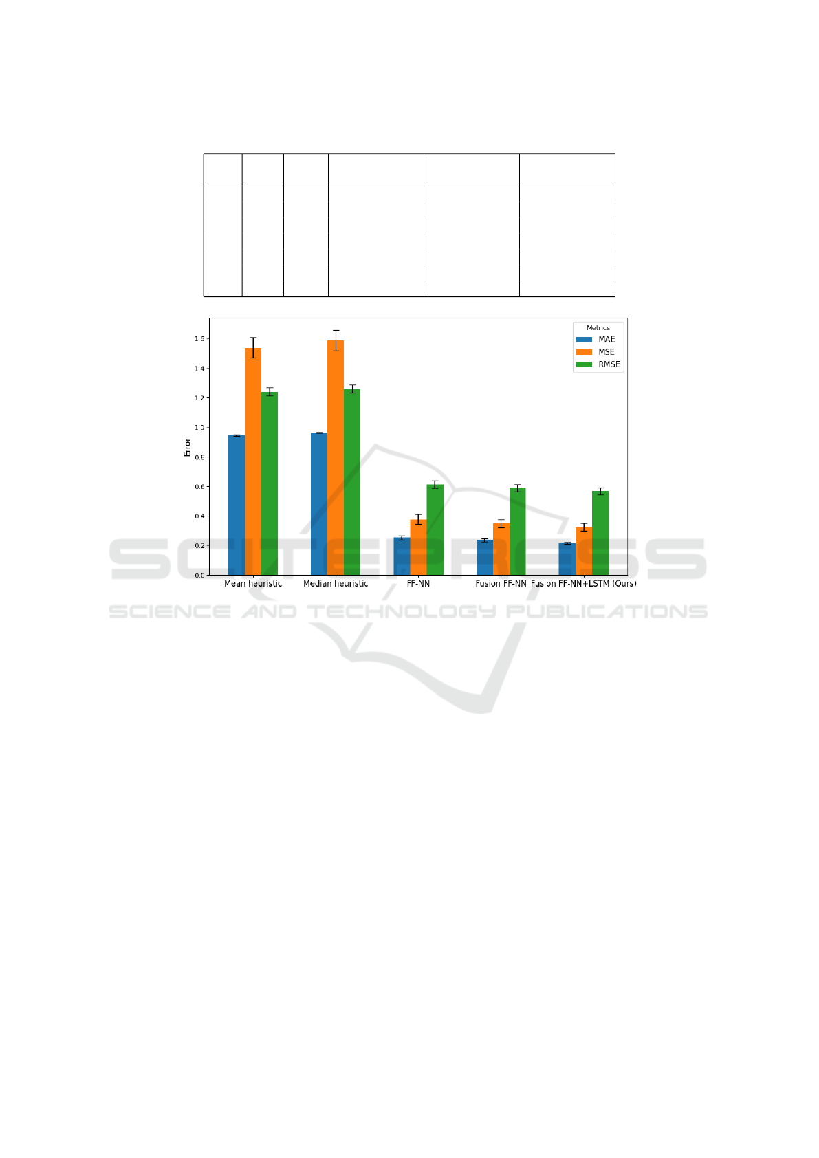
Table 2: The ablation study of the proposed method.
DM WM TFM
MAE
(µ ± σ)
MSE
(µ ± σ)
RMSE
(µ ± σ)
✓ 0.365 ± 0.011 0.950 ± 0.086 0.973 ± 0.021
✓ 0.243 ± 0.007 0.487 ± 0.050 0.697 ± 0.035
✓ 0.326 ± 0.021 0.466 ± 0.033 0.682 ± 0.024
✓ ✓ 0.233 ± 0.006 0.447 ± 0.046 0.668 ± 0.035
✓ ✓ 0.248 ± 0.006 0.396 ± 0.027 0.629 ± 0.022
✓ ✓ 0.220 ± 0.006 0.348 ± 0.021 0.590 ± 0.018
✓ ✓ ✓ 0.217 ± 0.006 0.325 ± 0.027 0.569 ± 0.024
Figure 5: Comparative analysis of the proposed method with the baselines as bar plots.
method, a degraded performance is observed where
MAE, MSE, and RMSE are reported as 0.365, 0.950,
and 0.973, respectively. When the settings with two
employed models are considered, the setting where
DM and WM are included improves performance in
all presented metrics for these settings with scores of
0.220, 0.348, and 0.590 for MAE, MSE, and RMSE,
respectively. Incorporating all models together with
a fusion model provides the best scores for all met-
rics with scores of 0.217, 0.325, and 0.569 for MAE,
MSE, and RMSE.
5 DISCUSSION AND
CONCLUSION
In this paper, we propose a traffic prediction method
based on historical density, tailored features, and
wave features. The proposed method utilizes distinct
models for each feature type, and fuses the outputs of
these models to predict the vessel traffic around the
vessel. Furthermore, the proposed model does not re-
quire a specific location representation, which makes
it applicable to any trajectory and processes generic
tailored features on the trajectory level, such as dis-
tance to the free sailing area and completeness ratio
of the voyage, to obtain generic insights related to the
location of the vessel. The proposed method is evalu-
ated on real-world AIS data and compared with base-
lines. The experimental results indicate that the per-
formance of the proposed method is promising, and it
outperforms the baselines.
5.1 Limitations
The method presented in this paper mainly consid-
ers historical density, sea conditions (i.e., wave) and
tailored features to predict traffic density for a given
trajectory. We are aware of the fact that it does not
consider potential real-time events, such as accidents,
which potentially affect the current vessel traffic at
sea. On the other hand, the proposed method provides
a forecast for the expected traffic along a trajectory,
which is an essential step toward safe navigation and
avoidance of delays or congestion.
ICAART 2025 - 17th International Conference on Agents and Artificial Intelligence
1060

The processed model requires features such as
planned speed or completeness ratio of the voyage,
and such features are obtained using passage plans.
In the absence of passage plans in the use of the
proposed method in real time, synthetic trajectories
can be obtained using reference trajectory algorithms,
which can then be used to predict traffic. Incorporat-
ing weather data, such as wind-related features, into
the presented feature set within an extensive dataset is
part of the future agenda.
ACKNOWLEDGEMENTS
This study has been funded by the Horizon Eu-
rope Research and Innovation program under grant
agreement No.101138478 and the Research Coun-
cil of Norway under grant agreement No. 346603,
the GASS project. The study has been conducted
using E.U. Copernicus Marine Service Information;
https://doi.org/10.48670/moi-00022. This work also
benefited from the Experimental Infrastructure for
Exploration of Exascale Computing (eX3), which
is financially supported by the Research Council of
Norway under contract number 270053. We thank
Joachim Berdal Haga and Thomas Roehr for their
contributions to implementing the density and tai-
lored features.
REFERENCES
Bodunov, O., Schmidt, F., Martin, A., Brito, A., and Fetzer,
C. (2018). Real-time destination and eta prediction for
maritime traffic. In Proceedings of the 12th ACM in-
ternational conference on distributed and event-based
systems, pages 198–201.
Dong, Z., Zhou, Y., and Bao, X. (2024). A short-term ves-
sel traffic flow prediction based on a dbo-lstm model.
Sustainability, 16(13):5499.
Hochreiter, S. (1997). Long short-term memory. Neural
Computation MIT-Press.
Huang, C., Chen, D., Fan, T., Wu, B., and Yan, X. (2024).
Incorporating environmental knowledge embedding
and spatial-temporal graph attention networks for in-
land vessel traffic flow prediction. Engineering Appli-
cations of Artificial Intelligence, 133:108301.
Li, Y., Liang, M., Li, H., Yang, Z., Du, L., and Chen, Z.
(2023). Deep learning-powered vessel traffic flow pre-
diction with spatial-temporal attributes and similarity
grouping. Engineering Applications of Artificial Intel-
ligence, 126:107012.
Liang, M., Liu, R. W., Zhan, Y., Li, H., Zhu, F., and Wang,
F.-Y. (2022). Fine-grained vessel traffic flow predic-
tion with a spatio-temporal multigraph convolutional
network. IEEE Transactions on Intelligent Trans-
portation Systems, 23(12):23694–23707.
Mandalis, P., Chondrodima, E., Kontoulis, Y., Pelekis, N.,
and Theodoridis, Y. (2024). A transformer-based
method for vessel traffic flow forecasting. GeoInfor-
matica, pages 1–25.
Parola, F., Satta, G., Notteboom, T., and Persico, L. (2021).
Revisiting traffic forecasting by port authorities in the
context of port planning and development. Maritime
Economics & Logistics, 23(3):444.
Perera, L. P. and Soares, C. G. (2017). Weather routing and
safe ship handling in the future of shipping. Ocean
Engineering, 130:684–695.
Rong, H., Teixeira, A., and Soares, C. G. (2022). Maritime
traffic probabilistic prediction based on ship motion
pattern extraction. Reliability Engineering & System
Safety, 217:108061.
Su, G., Liang, T., and Wang, M. (2020). Prediction of vessel
traffic volume in ports based on improved fuzzy neural
network. IEEE Access, 8:71199–71205.
Teng, T.-H., Lau, H. C., and Kumar, A. (2017). Coordinat-
ing vessel traffic to improve safety and efficiency. In
Proceedings of the 16th Conference on Autonomous
Agents and MultiAgent Systems, AAMAS ’17, page
141–149, Richland, SC.
Wan, Z., Chen, J., Makhloufi, A. E., Sperling, D., and Chen,
Y. (2016). Four routes to better maritime governance.
Nature, 540(7631):27–29.
Wang, D., Meng, Y., Chen, S., Xie, C., and Liu, Z. (2021).
A hybrid model for vessel traffic flow prediction based
on wavelet and prophet. Journal of Marine Science
and Engineering, 9(11):1231.
Wei, H., Cheng, Z., Sotelo, M., et al. (2017). Short-term
vessel traffic flow forecasting by using an improved
kalman model [j]. Cluster Computing, 23(10):1–10.
Xiao, H., Zhao, Y., and Zhang, H. (2022). Predict vessel
traffic with weather conditions based on multimodal
deep learning. Journal of Marine Science and Engi-
neering, 11(1):39.
Xiao, Z., Fu, X., Zhang, L., and Goh, R. S. M. (2019).
Traffic pattern mining and forecasting technologies in
maritime traffic service networks: A comprehensive
survey. IEEE Transactions on Intelligent Transporta-
tion Systems, 21(5):1796–1825.
Xie, Z. and Liu, Q. (2018). Lstm networks for vessel traffic
flow prediction in inland waterway. In 2018 IEEE In-
ternational Conference on Big Data and Smart Com-
puting (BigComp), pages 418–425.
Zhang, X., Fu, X., Xiao, Z., Xu, H., and Qin, Z.
(2022). Vessel trajectory prediction in maritime trans-
portation: Current approaches and beyond. IEEE
Transactions on Intelligent Transportation Systems,
23(11):19980–19998.
Zis, T. P., Psaraftis, H. N., and Ding, L. (2020). Ship
weather routing: A taxonomy and survey. Ocean En-
gineering, 213:107697.
Deep Learning-Based Vessel Traffic Prediction Using Historical Density and Wave Features
1061