Reconstruction of 3D Brain Structures from Clinical 2D MRI Data

Rui Shi

1 a

, Tsukasa Koike

2 b

, Tetsuro Sekine

3 c

, Akio Morita

4 d

and Tetsuya Sakai

1 e

Department of Computer Science and Engineering, Waseda University, Shinjuku, Tokyo, Japan

Department of Neurosurgery, Teraoka Memorial Hospital, Fukuyama, Hiroshima, Japan

Department of Radiology, Nippon Medical School Musashi Kosugi Hospital, Kawasaki, Kanagawa, Japan

Tokyo Rosai Hospital, Ota, Tokyo, Japan

Keywords:

Brain MRI, 3D Reconstruction.

Abstract:

As the population is aging worldwide, the number of dementia patients increases. Brain MRI is expected to

play a crucial role in the prediction of dementia at an early stage. Current 3D brain structure reconstruction

methods have strict rules and require a large number of slice images. Routine clinical MRI ﬁles contain much

fewer slices, but diagnosis relies heavily on information obtained from MRI scans. In this paper, we proposed

a method that is able to reconstruct the 3D brain structure with 2D DICOM MRI images within the clinical

routine budget, by applying trilinear interpolation. The generated images and structures are evaluated with

PSNR and SSIM. The results show that although the details in the generated 2D slices are not ideal, our

method is able to reconstruct 3D structures that are highly similar to the original brain structures using only

one-ﬁfth of the image slices.

1 INTRODUCTION

Population around the world is aging. For example,

in Japan, the proportion of people aged 65 and over

exceeds one-quarter of the total population (Statis-

tics Bureau, 2023). Providing proper medical care for

senior citizens is a major issue and needs to be ad-

dressed with contributions from society.

Dementia is one of the most common mental ill-

nesses that afﬂict the elderly, which causes a decline

in cognitive abilities and has negative impacts on the

individual in various ways, such as mobility, emotion,

and social relationships (van der Flier and Scheltens,

2005). Since dementia is slowly progressive (Bathini

et al., 2019), if diagnosed at the early stage, the devel-

opment of the disease can be eased with intervention.

Such prediction models are expected to be developed

with Brain MRI images.

Magnetic resonance imaging (MRI) technology

has been used for decades to obtain high-quality brain

images. Compared to other diagnostic imaging tech-

niques, MRI does not expose patients to radiation

in Positron Emission Tomography (PET) (Carlson

https://orcid.org/0009-0002-7339-0305

https://orcid.org/0000-0002-9931-0716

https://orcid.org/0000-0003-1547-6696

https://orcid.org/0000-0002-2497-5772

https://orcid.org/0000-0002-6720-963X

and Carlson, 2007), and provides better tissue con-

trast than Computed Tomography (CT) Scanner (Ebel

and Benz-Bohm, 1999). Various information can be

obtained through Brain MRI, such as the changes

in white matter which reﬂect systemic hypertension

(Salerno et al., 1992).

MRI scans divide the brain into slices at given in-

tervals, where each slice shows a 2D scan image of

the corresponding location. During the slicing pro-

cess, 3D characteristics of the patient’s brain can be

lost. The volume and proportions become difﬁcult to

quantify, and the spatial relationships between differ-

ent parts are unclear. But most current diagnoses and

surgery plans are based on MRI scans. Hence, it is

essential to reconstruct the 3D structure of the brain

for accurate presentation and alignment.

DICOM is the standard format used in hospitals

and clinics for MRI (Mustra et al., 2008). If the 3D

brain structure is reconstructed by simply stacking the

slice images according to their location, at least 100

slices are required for each coordinate axis, or a total

of more than 300. However, in clinical routine, DI-

COM MRI ﬁles are usually generated with only 19

slices along one single coordinate axis for ﬁnancial

and waiting time considerations. Diagnoses based on

such ﬁles highly depend on the expertise and experi-

ence of the doctor.

To ﬁll the gap and better assist doctors in diagno-

sis and surgery decisions, in this work, we propose a

352

Shi, R., Koike, T., Sekine, T., Morita, A. and Sakai, T.

Reconstruction of 3D Brain Structures from Clinical 2D MRI Data.

DOI: 10.5220/0013259000003905

Paper published under CC license (CC BY-NC-ND 4.0)

In Proceedings of the 14th International Conference on Pattern Recognition Applications and Methods (ICPRAM 2025), pages 352-359

ISBN: 978-989-758-730-6; ISSN: 2184-4313

method to reconstruct the 3D brain structure with 2D

MRI images at a relatively low cost, with a limited

number of slices within the clinical routine budget,

while aiming for high quality, accuracy, and speed.

2 PRELIMINARIES

2.1 Background

2.1.1 Metadata in DICOM Files

Each DICOM ﬁle has a metadata header, providing

information such as slice spacing and dimension. To

achieve success in 3D reconstruction by stacking the

2D slices, the required number of slices exceeds what

is obtained in most routine clinical MRI DICOM ﬁles,

and the metadata of the slices must match in a highly

accurate order (AlZu’bi et al., 2020). However, vibra-

tion during the scan process and variations between

acquisition devices can lead to divergences and inac-

curacies in the metadata.

In addition, routine clinical MRI slices are mostly

separated with relatively large spacing, leaving the

structures between the intervals vacant. By simply

stacking the images, the generated structure is discon-

tinuous because of the information lost in the inter-

vals, and differs largely from the actual structure.

2.1.2 Bias Field and Noise

Bias ﬁeld exists during MRI scans, especially those

taken by old MRI machines. Such uneven intensity

produces smooth, low-frequency signals that interfere

with the MRI scanning process (Juntu et al., 2005).

Bias ﬁeld can cause intensity variation among homo-

geneous tissues, which changes high-frequency com-

ponents such as contours and edges, causing blurs in

the images. The variation may not be easily observed

but can result in the decline of feature points during

image processing.

Also, the RF emission from the thermal mo-

tion of the patient’s body causes much inevitable

noise in the scanned MRI images, which appears

as irregular granular patterns and confuses informa-

tion acquisition (Aja-Fern

andez and Vegas-S

anchez-

Ferrero, 2016).

2.2 Related Work

2.2.1 Pre-Processing of Image

Histogram equalization is often used to counteract the

effects of bias ﬁelds (Senthilkumaran and Thimmi-

araja, 2014). It is a general method used for grayscale

image enhancement, performed with the cumulative

distribution function (CDF) of intensity. Since image

voxels in DICOM ﬁles are encoded by intensity, they

resemble the grayscale images, which share the same

color channel. The images processed by histogram

equalization will have higher contrast than the origi-

nal images.

Noise ﬁlters are also widely used to improve the

quality of scanned images. There are various types of

noise ﬁlters, realized with different approaches. For

example, in the work of Thanh and Hai (Thanh and

Hai, 2017), a mean-unsharp ﬁlter, which is convo-

luted with the 2D MRI images, is applied to remove

the noise.

2.2.2 Marching Cube

Marching cubes is a classic computer graphics algo-

rithm that can produce high-resolution 3D surfaces

with simple construction operations (Lorensen and

Cline, 1998). Even in recent years, this algorithm has

shown good performance in reconstructing 3D knee

surfaces and spine structures from 2D CT images (Pa-

tel and Mehta, 2012), but the calculation will be slow

if a large amount of 2D data is processed.

2.2.3 Interpolation

Interpolation is a mathematical approach to estimate

unknown points based on the existing points. By con-

structing a continuous function that passes through

the given data points, unknown points between the

given data points can be approximated with a high ac-

curacy (Davis, 1975). In Ghoshal’s work (Ghoshal

et al., 2020), highly accurate 3D reconstruction of

spine is achieved by combining the Marching cubes

algorithm and interpolation. Although not quantiﬁed,

reconstruction works of 3D brain structure from 2D

MRI images have also received satisfying results us-

ing trilinear interpolation (Fajar et al., 2022) (Thanh

and Hai, 2017).

3 METHOD

In this section, we propose a method that is able to re-

construct the 3D brain structure from a small amount

of 2D DICOM MRI images along one single coordi-

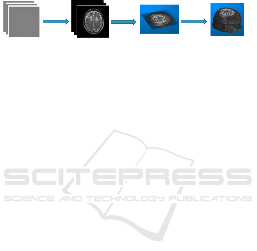
nate axis. Figure 1 shows the four steps taken to ac-

complish the process, which are introduced in detail.

3.1 Pre-Processing of Image

We propose two alternative approaches for contrast

enhancement and noise cancellation. Approach A in-

Reconstruction of 3D Brain Structures from Clinical 2D MRI Data

353

Original image slices

T2 (Axial)

- Case 1 2007/03/30 from the Test Dataset

Image slices after Pre-processing

Resized Reconstructed 3D structure

with transparent background

Step 1

Step 2

Primitive Reconstructed 3D

Structure

Step 3 & 4

Figure 1: Workﬂow of 3D Brain Reconstruction from Clinical 2D MRI Image data. 1) Pre-processing of the image; 2)

Reconstruction of 3D structure with Trilinear Interpolation; 3) Resizing the generated 3D Image; 4) Making the Background

Transparent. The demonstrated original images are from the MRI record collected on Patient Case 1 from the Test Dataset on

March 30, 2007. Further information on the Test Dataset can be found in Section 4.

volves histogram equalization and a noise ﬁlter, while

Approach B comprises only one contrast ﬁlter.

3.1.1 Histogram Equalization

Histogram equalization is applied to enhance the

contrast in the images. Considering in a discrete

grayscale image x, the probability of the occurrence

of a pixel of level i in the image is:

(i) = p(x = i) =

, 0 ≤ i < L (1)

where L is the maximum pixel value, n

is the

number of occurrences of the pixel of level i, and n

is the number of pixels in the image.

As an MRI DICOM image is similar to a grayscale

image with intensity ranging from 0 to 255 for every

voxel, L equals the intensity level bound 256. The

CDF for the intensity v can be calculated as

cdf

(v) =

∑

j=0

(x = j) (2)

The histogram-equalized intensity value h(v) is

derived as

h(v) = round(cdf

(v) · (L − 1)) (3)

Through histogram equalization, the equalized in-

tensity value replaces the original value, distribut-

ing the pixels more evenly throughout the full range,

which gives the image a higher contrast.

3.1.2 Noise Filter

Our noise ﬁlter is developed with homogenization of

the background.

First, we verify the boundary of the skull. As the

objects within the head are separated from the back-

ground by the skull, which preserves a much brighter

shade than the surrounding background, we can eas-

ily measure the intensity value of the skull and set the

value as a threshold.

Once the threshold is obtained, the head boundary

can be detected. The noise or irrelevant background

can be effectively removed by setting all pixels out-

side the identiﬁed boundaries to zero.

3.1.3 Contrast Filter

An alternative way to enhance the contrast and cancel

the noise in one step is to use a contrast ﬁlter. We de-

signed a contrast ﬁlter that adjusts the image contrast

by normalizing the pixel values to the full 8-bit range

0 to 255.

First, we ﬁnd the maximum and minimum pixel

values in the image, and calculate the range of vari-

ance in pixel value by subtracting the minimum value

from the maximum value.

Then, we subtract the minimum pixel value from

each pixel and divide the subtraction results by the

range of pixel value variance to normalize the pixel

values to 0 to 1.

Finally, we multiply the division results by 255 to

scale the normalized values into 0 to 255.

Through the contrast ﬁlter, the pixels are dis-

tributed more evenly to the full range, and the abrupt

variance caused by noise is also mostly reduced, can-

celing noise during the normalization process.

3.2 Reconstruction of 3D Structure with

Trilinear Interpolation

After pre-processing, the 2D image slices are now

ready to be primitively combined to form the 3D

structure.

First, the 2D image slices are stacked according

to their slice location shown in the metadata. When

image data are simply stacked, there is much empty

space with missing information at the intervals be-

tween the slices. As the intervals are large for routine

clinical MRI images, the spacing may vary between

slices.

These empty intervals can be ﬁlled with the slices

generated by trilinear interpolation, which recon-

structs the 3D information between the slices and

smoothens the structure. The aim is to approximate

ICPRAM 2025 - 14th International Conference on Pattern Recognition Applications and Methods

354

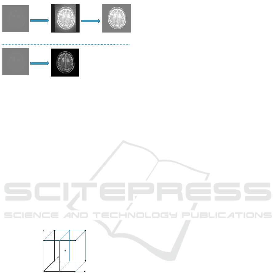
Image after histogram

equalization

Denoised image after

histogram equalization

Image after our

contrast filter

Original image

slices

T2 (Axial)

- Case 1 2007/03/30

Histogram

equalization

Noise Filter

Contrast

filter

Approach A

Approach B

Original image

slices

T2 (Axial)

- Case 1 2007/03/30

Figure 2: Workﬂows of the Alternative Approaches (Ap-

proach A and Approach B) for Contrast Enhancement and

Noise Cancellation. Approach A ﬁrst applies Histogram

Equalization to the original image, then passes the equal-

ized image through the Noise Filter. Approach B only

passes the original image through the Contrast Filter. The

demonstrated original image is one slice from the MRI

record collected on Patient Case 1 from the Test Dataset

on March 30, 2007.

the original 3D structures with our interpolated struc-

tures.

Trilinear interpolation is a method of multivariate

interpolation on a 3D regular grid (Davis, 1975). It

can predict the pixel value of any point within the 3D

structure with a faster speed than the Marching cube

(Rajon and Bolch, 2003), as follows:

Considering in a unit-size cubic lattice, a point lo-

cated at (u, v, w) in the spatial domain expects pixel

prediction by trilinear interpolation, as shown in 3.

(u,v,w)

Figure 3: An example of Trilinear Interpolation within a

unit-size cubic lattice. The 3D Cartesian coordinate system

is formed by the x, y, and z axes. The C

values are the pixel

values of the vertices, where n is the index for each vertex.

The point located at (u, v, w) is expecting pixel prediction.

The pixel value C(u, v, w) of the point located at

(u, v, w) is calculated as:

C(u, v, w)

(1 − u)(1 − v)(1 − w) +C

u(1 − v)(1 − w)

uv(1 − w) +C

(1 − u)v(1 − w)

(1 − u)(1 − v)w +C

u(1 − v)w

uvw +C

(1 − u)vw

(4)

3.3 Resizing 3D Image

The default setting makes the primitive reconstructed

3D structure a plate. Therefore, resizing is needed

to adjust the structure to the proper scale. We adjust

the proportions of the head referencing biostatistics

data (Bail et al., 2009) and uniformize the size and

resolution of the generated 3D brain structures.

3.4 Making the Background

Transparent

During the pre-processing step, we evenly enhanced

the image contrast, where the pixels representing the

objects within the head preserved a much different

intensity level from the pixels representing the back-

ground. We can set the pixels within the background

level to 0 to make the background transparent eas-

ily and efﬁciently, so that the brain structure can be

clearly viewed from all angles and is emphasized.

4 EXPERIMENT

In this section, the details of our experiments are clar-

iﬁed.

4.1 Dataset

In this research, we use a Test Dataset and an Eval-

uation Dataset. Both datasets are collected from the

Teraoka Memorial Hospital in Hiroshima, Japan.

4.1.1 Test Dataset

The Test Dataset consists of 115 records of 2D MRI

DICOM ﬁles. Nineteen volunteers have contributed

to this dataset through the years.

Each 2D MRI DICOM ﬁle in this dataset includes

19 slices at a spacing interval of 5 mm. There are

three types of data scanned along the coordinate axes:

(1) The Axial data is collected along the vertical axis,

from the top to the bottom of the head; (2) The Coro-

nal data is collected along one horizontal axis, from

the back to the front of the head; (3) The Sagittal data

is collected along the other horizontal axis, orthogo-

nal to the Coronal axis, from the side of the head.

This dataset is used to verify whether our method

is adaptable to all kinds of data, as there is a relatively

rich number of samples and a variety of data types in

this dataset.

Reconstruction of 3D Brain Structures from Clinical 2D MRI Data

355

4.1.2 Evaluation Dataset

The Evaluation Dataset consists of 22 records of 3D

MRI DICOM ﬁles for evaluation. This dataset is con-

tributed by twenty-two volunteers.

In this dataset, there are 22 records of 3D Sagittal

data. Each record of such data includes approximately

100 slices, spaced with an interval of 1 mm.

This dataset is used to evaluate the generation per-

formance quantitatively. With this dataset, by taking

samples from the 3D Sagittal data, we can not only

obtain the similarity of the entire structure between

the original form and the generated form, but also the

similarity between the generated slice and the origi-

nal slice. In addition, if we take the ﬁrst slice in every

ﬁve slices as a sample, we can create a sampled 2D

set containing approximately 20 slices, similar to the

routine clinical ﬁle containing 19 slices. Hence, we

can expect similar performance in reconstructing 3D

brain structure using the proposed method, with rou-

tine clinical MRI data.

4.2 Evaluation Metrics

Two evaluation metrics are applied to validate the re-

sults.

4.2.1 Peak Signal to Noise Ratio (PSNR)

Peak signal-to-noise ratio (PSNR) is an image eval-

uation measure. It is often used to calculate the vi-

sual error between two images, such as measuring the

visual difference between the original image and the

compressed image, the difference between the image

generated by the generative network and the actual

image, etc.

PSNR is deﬁned via the mean squared error

(MSE). Suppose there are two m×n monochrome im-

ages I and K, I is noiseless and K is similar to I but

contains noise. MSE between I and K is deﬁned as

MSE(I, K) =

m−1

∑

i=0

n−1

∑

j=0

[I(i, j) − K(i, j)]

(5)

where I(i, j) and K(i, j) are the pixel values at posi-

tion (i, j) (i-th row and j-th column) in I and K re-

spectively.

PSNR is deﬁned in units of dB, as

PSNR(I, K) = 10 · log

(MAX

)

MSE

(6)

where MAX

is the maximum pixel value of the orig-

inal image.

PSNR is always non-negative and equals inﬁnity

when the two images are identical (Bull and Zhang,

2014). The higher the PSNR value, the less noise in

the noisy image. PSNR is a pixel-wise metric: if the

pixel value is different, it will be considered as noise

and quantiﬁed.

4.2.2 Structural Similarity Index Measure

(SSIM)

Structural similarity index measure (SSIM) is an-

other metric for measuring the similarity between

two images. SSIM performs the comparison from

a structural perspective, considering brightness, con-

trast, and structural information in the images (Wang

et al., 2004). Structural information assumes that pix-

els have strong inter-dependencies, especially when

spatially close.

Suppose there are two images x and y, SSIM be-

tween x and y is deﬁned as

SSIM(x, y) = [l(x, y)]

[c(x, y)]

[s(x, y)]

(7)

where

l(x, y) =

2µ

(µ

)

+(µ

)

compares the brightness

between x and y;

c(x, y) =

2σ

(σ

)

+(σ

)

compares the contrast be-

tween x and y;

s(x, y) =

compares the structure similarity

between x and y;

α, β, γ are the positive parameters for adjustment;

, µ

are the pixel sample means of x and y;

, σ

are the standard deviations of x and y;

is the covariance of x and y;

are constants to stabilize the division

with a weak denominator.

The higher the SSIM value is, the higher the sim-

ilarity the two images preserve. The maximum value

of SSIM is achieved when the two images are iden-

tical, and the SSIM value can be negative when the

structural information in the two images differs too

much.

5 RESULTS

In Section 2, we proposed two alternative approaches

for pre-processing. Figure 4 shows the processed im-

ages for a record with Approaches A and B, respec-

tively.

Both the original and the generated 3D brain struc-

ture can be presented and observed from all angles af-

ter the execution of the implemented program. Figure

5 shows a sample of the original and the generated 3D

brain structures from the same record.

ICPRAM 2025 - 14th International Conference on Pattern Recognition Applications and Methods

356

(a) Denoised image after his-

togram equalization.

(b) Image after our contrast

ﬁlter.

Figure 4: The 2D MRI images pre-processed with alterna-

tive approaches for Contrast Enhancement and Noise Can-

cellation. (a) Approach A, ﬁrst applying Histogram Equal-

ization to the original image, and then passing the equalized

image through the Noise Filter. (b) Approach B, which only

passes the original image through the Contrast Filter. The

demonstrated images came from the same original image,

one slice from the MRI record collected on Patient Case 1

from the Test Dataset on March 30, 2007.

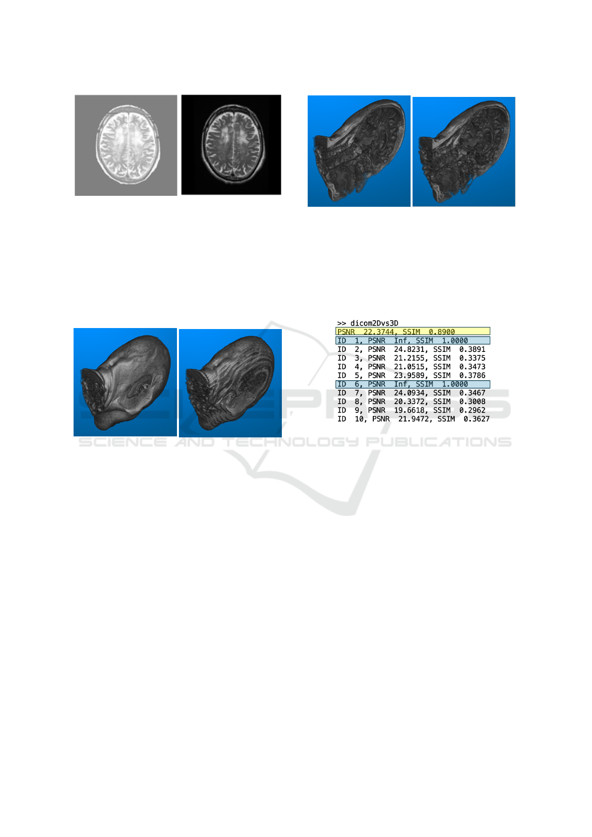
(a) Original structure.

(b) Generated structure.

Figure 5: An example of the Original and the Generated

3D Brain Structures from the Same Record. The left di-

agram shows the original 3D brain structure stacked with

103 slices along the corresponding axis. The right diagram

shows the interpolated 3D brain structure generated with 21

sampled slices along the same axis. The image data used by

both diagrams came from the same MRI record collected on

Patient Case 01 from the Evaluation Dataset.

Cross-sections can also be cut at arbitrary posi-

tions in the original and the generated 3D brain struc-

ture, allowing observation from all angles. Figure 6

shows a sample of the original and the generated 2D

brain slices from the same record.

Calculation results of the PSNR and SSIM val-

ues are printed out after execution of the implemented

program. Figure 7 presents an example showing part

of the output.

The average PSNR and SSIM results for each

patient are summarized in Table 1. The PSNR and

SSIM (Structure) values are obtained by comparing

the original and the generated 3D brain structures.

The SSIM (Slices) values are obtained by comparing

slice by slice.

(a) Original structure. (b) Generated structure.

Figure 6: An example of the Original and the Generated 2D

Brain Slices from the Same Record. The left diagram shows

a cross-section in the original 3D brain structure, while the

right diagram shows the cross-section at the same position,

from the same angle, in the interpolated 3D brain structure.

The image data used by both diagrams came from the same

MRI record collected on Patient Case 01 from the Evalua-

tion Dataset.

Figure 7: An example showing partial output. The values in

the yellow-marked area are obtained by comparing the orig-

inal and the generated 3D brain structures as an overview.

The rest of the output with IDs are obtained by making the

comparison slice by slice, between the original slices and

the corresponding slices at the same position from the inter-

polated 3D brain structure. The values in the blue-marked

areas are the results of the sampled slices. These results are

excluded from the statistical analysis later on. This output is

generated based on the data from the MRI record collected

on Patient Case 01 from the Evaluation Dataset.

6 DISCUSSION

6.1 Approach for Pre-Processing

Qualitatively, the image after our contrast ﬁlter pre-

served distinctively more complete objects and shows

higher contrast. On the contrary, the denoised image

has a lower contrast after histogram equalization, and

the objects have missing parts.

Hence, Approach B, which applies our contrast

ﬁlter, is chosen and used for the pre-processing.

Reconstruction of 3D Brain Structures from Clinical 2D MRI Data

357

Table 1: Average PSNR and SSIM results for each patient

from the Evaluation Dataset.

Patient No. PSNR

SSIM SSIM

(Structure) (Slices)

01 22.3744 0.8900 0.5686

02 22.3910 0.8781 0.5633

03 21.3912 0.8632 0.5398

04 21.9015 0.8878 0.5623

06 23.3431 0.8752 0.5476

08 22.0405 0.8249 0.5362

09 22.3152 0.8981 0.5854

010 23.0736 0.8863 0.5773

012 22.6628 0.8423 0.5405

S1 22.8207 0.8808 0.5883

S2 22.5581 0.8906 0.5692

S3 22.2656 0.8381 0.5102

S4 24.0652 0.8618 0.5719

S5 23.0599 0.8792 0.5344

S6 20.7212 0.7676 0.5241

S7 19.3878 0.7326 0.4919

S8 22.5163 0.8869 0.5752

S9 24.1441 0.8653 0.5427

S13 22.7782 0.8797 0.5608

S14 22.4127 0.8727 0.5385

S15 22.3385 0.8202 0.5078

S16 23.3206 0.8918 0.5401

Mean 22.4492 0.8597 0.5489

Variance 1.0060 0.0017 0.0006

6.2 Adaptability, Stability and

Computational Speed

The proposed method shows high adaptability, suc-

ceeding in 3D brain structure generation based on all

three types of data scanned along different coordinate

axes in the Test Dataset, with images containing ap-

proximately 20 slices.

Performance stability can be perceived from 5b:

despite some deviations among the patient cases in

PSNR, only minor variance appears in SSIM (Struc-

ture) and SSIM (Slices) measurement.

The computation is also efﬁcient. The average

time to generate the original 3D structure and the

reconstructed structure, and compute the PSNR and

SSIM values is within 2 seconds.

6.3 Pixel Similarity

The pixel similarity between the generated and the

original 3D structure is reﬂected by PSNR. The aver-

age PSNR value among all 22 cases of patients in the

Evaluation Dataset equals 22.45. Typical values for

the PSNR in lossy image and video compression are

between 30 and 50 dB, the higher the PSNR value, the

better quality the noisy image has (Faragallah et al.,

2020). Since there are fewer reference points in the

interpolation-generated images, the PSNR values are

generally lower (Jung and Yoo, 2009). Furthermore,

the objects inside the brain mainly consist of soft tis-

sues, which can be in small scales and various shapes,

yet have complicated spatial relationships (adjacent

and overlapping) (Nowinski, 2011). Considering the

delicacy of the brain structure, the obtained PSNR re-

sult and thus the pixel similarity are acceptable.

6.4 Structural Similarity

The structural similarity between the generated and

the original 3D structure is shown by SSIM (Struc-

ture). The average SSIM among the patients in the

Evaluation Dataset is 85.97%, with a minor vari-

ance of 0.2%. This indicates that the generated brain

structure can stably achieve 85.97% similarity to the

original 3D brain structure consisting of a relatively

large number of images (approx. 100), based on only

relatively few images (approx. 20, one-ﬁfth of the

ground-truth). This achievement can be considered

inspiring.

The structural similarity between the generated

and the original 2D slices is reﬂected by SSIM (Slice).

The average SSIM among the patients is 54.89%,

along with a minor variance of 0.1%. This indicates

that the generated image slices can stably achieve

54.89% similarity to the original slices at the same

position. Unlike the remarkable resemblance in the

overview of the 3D structure, in a 2D slice perspec-

tive, the generated images lack much more similarity

to the original slices.

One possible explanation for the gap between the

2D and 3D performance could be that, although the

sampled data has large spacing intervals between the

slices, the slices still manage to cover the information

for the entire brain, among which the major charac-

teristics that matter in the 3D structure are still pre-

served. However, linear prediction cannot precisely

regenerate the details on a 2D slice within the empty

intervals, with limited information of that localized

area being only two adjacent slices.

7 CONCLUSION

We proposed a low-cost method to reconstruct the 3D

brain structure with routine clinical 2D MRI images,

using trilinear interpolation. The results indicate that

our method delivers good performance in 3D brain

structure reconstruction, achieving a similarity of up

ICPRAM 2025 - 14th International Conference on Pattern Recognition Applications and Methods

358

to 85.97% between the original and the generated 3D

structure, using only one-ﬁfth of the required amount

of images for the traditional stacking method.

As future work, to obtain better pixel resemblance

and more details in the generated 2D slices, further

improvement can be made with techniques such as

combinations of algorithms and assistance from neu-

ral networks. In the near future, our method may as-

sist doctors in making more precious diagnoses and

better treatments for diseases and injuries, even con-

quering dementia.

REFERENCES

Aja-Fern

andez, S. and Vegas-S

anchez-Ferrero, G. (2016).

Statistical analysis of noise in mri. Switzerland:

Springer International Publishing.

AlZu’bi, S., Shehab, M., Al-Ayyoub, M., Jararweh, Y., and

Gupta, B. (2020). Parallel implementation for 3d med-

ical volume fuzzy segmentation. Pattern Recognition

Letters, 130:312–318.

Bail, L. et al. (2009). The Human Head A Correct De-

lineation of the Anatomy, Expressions, Features, Pro-

portions and Positions of the Head and Face. Tom

Richardson.

Bathini, P., Brai, E., and Auber, L. A. (2019). Olfactory

dysfunction in the pathophysiological continuum of

dementia. Ageing research reviews, 55:100956.

Bull, D. R. and Zhang, F. (2014). Digital picture formats

and representations. Communicating pictures, pages

99–132.

Carlson, N. R. and Carlson, N. R. (2007). Physiology of

behavior. Pearson Boston.

Davis, P. J. (1975). Interpolation and approximation.

Courier Corporation.

Ebel, K.-D. and Benz-Bohm, G. (1999). Differential diag-

nosis in pediatric radiology. Thieme.

Fajar, A., Sarno, R., Fatichah, C., and Fahmi, A. (2022). Re-

constructing and resizing 3d images from dicom ﬁles.

Journal of King Saud University-Computer and Infor-

mation Sciences, 34(6):3517–3526.

Faragallah, O. S., El-Hoseny, H., El-Shafai, W., Abd El-

Rahman, W., El-Sayed, H. S., El-Rabaie, E.-S. M.,

Abd El-Samie, F. E., and Geweid, G. G. (2020). A

comprehensive survey analysis for present solutions

of medical image fusion and future directions. IEEE

Access, 9:11358–11371.

Ghoshal, S., Banu, S., Chakrabarti, A., Sur-Kolay, S., and

Pandit, A. (2020). 3d reconstruction of spine image

from 2d mri slices along one axis. IET Image Pro-

cessing, 14(12):2746–2755.

Jung, K.-H. and Yoo, K.-Y. (2009). Data hiding method

using image interpolation. Computer Standards & In-

terfaces, 31(2):465–470.

Juntu, J., Sijbers, J., Van Dyck, D., and Gielen, J. (2005).

Bias ﬁeld correction for mri images. In Computer

Recognition Systems: Proceedings of the 4th Interna-

tional Conference on Computer Recognition Systems

CORES’05, pages 543–551. Springer.

Lorensen, W. E. and Cline, H. E. (1998). Marching cubes:

A high resolution 3d surface construction algorithm.

In Seminal graphics: pioneering efforts that shaped

the ﬁeld, pages 347–353.

Mustra, M., Delac, K., and Grgic, M. (2008). Overview of

the dicom standard. In 2008 50th International Sym-

posium ELMAR, volume 1, pages 39–44. IEEE.

Nowinski, W. L. (2011). Introduction to brain anatomy.

Biomechanics of the Brain, pages 5–40.

Patel, A. and Mehta, K. (2012). 3d modeling and rendering

of 2d medical image. In 2012 International Confer-

ence on Communication Systems and Network Tech-

nologies, pages 149–152. IEEE.

Rajon, D. A. and Bolch, W. E. (2003). Marching cube algo-

rithm: review and trilinear interpolation adaptation for

image-based dosimetric models. Computerized Medi-

cal Imaging and Graphics, 27(5):411–435.

Salerno, J. A., Murphy, D., Horwitz, B., DeCarli, C.,

Haxby, J. V., Rapoport, S. I., and Schapiro, M. B.

(1992). Brain atrophy in hypertension. a volumet-

ric magnetic resonance imaging study. Hypertension,

20(3):340–348.

Senthilkumaran, N. and Thimmiaraja, J. (2014). Histogram

equalization for image enhancement using mri brain

images. In 2014 World congress on computing and

communication technologies, pages 80–83. IEEE.

Statistics Bureau (2023). Population and households. In

JAPAN STATISTICAL YEARBOOK 2024, chapter 2,

pages 29–82. Ministry of Internal Affairs and Com-

munications, Tokyo.

Thanh, C. Q. and Hai, N. T. (2017). Trilinear interpolation

algorithm for reconstruction of 3d mri brain image.

American Journal of Signal Processing, 7(1):1–11.

van der Flier, W. M. and Scheltens, P. (2005). Epidemiology

and risk factors of dementia. Journal of Neurology,

Neurosurgery & Psychiatry, 76(suppl 5):v2–v7.

Wang, Z., Bovik, A. C., Sheikh, H. R., and Simoncelli, E. P.

(2004). Image quality assessment: from error visi-

bility to structural similarity. IEEE transactions on

image processing, 13(4):600–612.

Reconstruction of 3D Brain Structures from Clinical 2D MRI Data

359