Oil Spill Segmentation Using Deep Encoder-Decoder Models

Abhishek Ramanathapura Satyanarayana

and Maruf A. Dhali

Department of Artiﬁcial Intelligence, Bernoulli Institute, University of Groningen, 9747 AG Groningen, The Netherlands

Keywords:

Oil Spill, Semantic Segmentation, Neural Networks, Deep Learning.

Abstract:

Crude oil is an integral component of the world economy and transportation sectors. With the growing demand

for crude oil due to its widespread applications, accidental oil spills are unfortunate yet unavoidable. Even

though oil spills are difﬁcult to clean up, the ﬁrst and foremost challenge is to detect them. In this research, the

authors test the feasibility of deep encoder-decoder models that can be trained effectively to detect oil spills

remotely. The work examines and compares the results from several segmentation models on high dimensional

satellite Synthetic Aperture Radar (SAR) image data to pave the way for further in-depth research. Multiple

combinations of models are used to run the experiments. The best-performing model is the one with the

ResNet-50 encoder and DeepLabV3+ decoder. It achieves a mean Intersection over Union (IoU) of 64.868%

and an improved class IoU of 61.549% for the “oil spill” class when compared with the previous benchmark

model, which achieved a mean IoU of 65.05% and a class IoU of 53.38% for the “oil spill” class.

1 INTRODUCTION

Seas, oceans, and coastal regions represent vital com-

ponents of the environment, marine ecosystems, and

human activities. The aquatic ecosystem is a crucial

source of economic stability and livelihoods for a sig-

niﬁcant portion of the global population. However,

numerous human activities pose substantial threats to

marine ecosystems, with oil spills being a notable

one. These spills can arise from various sources, in-

cluding the transportation of crude oil. Crude oil is

integral to many industrial and manufacturing pro-

cesses, ﬁnding application in sectors such as gasoline,

diesel, jet fuel, lubricants, textiles, paint, fertilizers,

pesticides, and pharmaceuticals, serving as a critical

driver of industrial development and expansion. How-

ever, the primary method of transporting crude oil

globally is through shipping tankers, which inevitably

leads to accidental oil spills. Apart from accidental

oil spills, other causes may include incidents from

offshore platforms, drilling rigs and wells, natural

disasters, deliberate releases, and technical failures.

These events can lead to catastrophic environmental

impacts, adverse human health effects, and signiﬁ-

cant socio-economic consequences. Additionally, oil

spills can severely affect wildlife, including birds and

marine mammals, disrupting ecosystems and leading

https://orcid.org/0009-0003-1248-0988

https://orcid.org/0000-0002-7548-3858

to long-term ecological damage (Dunnet et al., 1982).

Besides affecting marine ecosystems, it also affects

the air quality (Middlebrook et al., 2010). Oil spills

have faced signiﬁcant public and media backlash due

to their harmful effects, prompting political and gov-

ernmental institutions to prevent future occurrences

(Broekema, 2016). Oil spills may take a long time to

clean up, and the duration can vary signiﬁcantly de-

pending on several factors, including the spill’s size,

the type of oil, environmental conditions, and the ef-

fectiveness of the response efforts (Shigenaka, 2009).

It is essential to automatically and efﬁciently detect

oil spills to enable prompt action for containment and

cleanup. One effective approach is to combine remote

sensing with artiﬁcial intelligence and supervised ma-

chine learning models speciﬁcally trained to identify

spills. Remote sensing can be accomplished through

satellite imagery for this purpose. Recently, there

has been a growing interest in using deep Convolu-

tional Neural Networks (CNNs) to process this im-

age data. The introduction of the AlexNet model has

demonstrated signiﬁcant performance improvements

over traditional feature engineering techniques, par-

ticularly in the ImageNet object recognition compe-

tition. (Deng et al., 2009; Russakovsky et al., 2015;

Krizhevsky et al., 2012). Earlier works have utilized

CNN models to detect oil spills using Synthetic Aper-

ture Radar (SAR) satellite imagery. Marios Kresteni-

tis et al. applied some modiﬁcations and trained some

Satyanarayana, A. R. and Dhali, M. A.

Oil Spill Segmentation Using Deep Encoder-Decoder Models.

DOI: 10.5220/0013259600003905

Paper published under CC license (CC BY-NC-ND 4.0)

In Proceedings of the 14th International Conference on Pattern Recognition Applications and Methods (ICPRAM 2025), pages 741-748

ISBN: 978-989-758-730-6; ISSN: 2184-4313

741

of the CNN models to detect oil spills in their research

(Krestenitis et al., 2019). They divided the origi-

nal high-dimensional images into smaller patches and

trained various models on these. This process may

consume a signiﬁcant amount of memory, necessi-

tating extensive computing resources and resulting

in increased energy usage. As technology advances,

developing and training models directly on higher-

dimensional images is essential to achieve better per-

formance. This can help reduce the memory required

for processing by a certain amount, reducing the en-

ergy required for computation. In this research, an

attempt is made to train various CNN models on rela-

tively higher dimensional images and study the effects

on the overall performance of the models.

2 RELATED WORKS

With the emergence of Artiﬁcial Neural Networks

(ANNs), Yann LeCun et al. proposed LeNet-5, the

ﬁrst Convolutional Neural Network (CNN), that was

applied to the image digit recognition task (LeCun

et al., 1989; LeCun et al., 1998). Later, a popu-

lar dataset — the MNIST dataset became a bench-

mark for the digit recognition task in images (Deng,

2012). There was a signiﬁcant gap in the applica-

tion of CNNs to various Computer Vision and Im-

age Analysis tasks for multiple reasons, with a lack

of computation power and a lack of large-scale la-

beled datasets being a few among them. Recently, Im-

ageNet has been hosting an object recognition chal-

lenge on a large-scale dataset (Deng et al., 2009;

Russakovsky et al., 2015). This dataset consists of

1.2 million images belonging to 1000 classes. In

2012, a CNN model named AlexNet won the Ima-

geNet object recognition challenge, outperforming all

the other participants of that year by a large margin

(Krizhevsky et al., 2012). The other participants used

non-CNN methods, i.e., the traditional handcrafted

features combined with different machine learning

techniques. One key challenge in computer vision is

semantic segmentation, where the model must learn

to classify each pixel in an image into a speciﬁc cate-

gory. In 2014, Jonathan Long et al. proposed a Fully

Convolutional Network (FCN), which was the ﬁrst

CNN with only convolutional and transposed convo-

lutional layers and without any fully connected (or

dense) layers (Long et al., 2014). With the advent

of FCNs, researchers have proposed and developed

several other state-of-the-art models for the semantic

segmentation task. Among them, the popular ones

include — UNet, LinkNet, PSPNet, DeepLabV3+

(Ronneberger et al., 2015; Chaurasia and Culurciello,

2017; Zhao et al., 2016; Chen et al., 2018). These

models have one thing in common — i.e., they are

all variations of encoder-decoder architectures. Most

of these models have been benchmarked on large

datasets such as COCO and Cityscapes (Lin et al.,

2014; Cordts et al., 2016). Cityscapes, a labeled

dataset used as a benchmark for semantic segmenta-

tion tasks, contains 5000 high quality labeled images

and 20000 weakly labeled images. Marios Kresteni-

tis et al. benchmarked some of these models on

the Oil Spill Detection Dataset, a dataset developed

by compiling the images extracted from the satel-

lite Synthetic Aperture Radar (SAR) data (Kresteni-

tis et al., 2019). This dataset contains a meager

1002 training image, which is relatively much lower

than the Cityscapes dataset. In their research, Mar-

ios Krestenitis et al. trained the models by divid-

ing the original images of size 1250 × 650 into mul-

tiple patches. They used the image patches as in-

put for the models. They used different image patch

sizes for various models. Although different encoders

were used in the original implementations of these

models, Marios Krestenitis et al. modiﬁed the mod-

els to use ResNet-101 encoder for most of the de-

coders, the exception being MobileNetV2 encoder

with DeepLabV3+ decoder in their research (He et al.,

2015; Krestenitis et al., 2019; Chen et al., 2018; San-

dler et al., 2018). Their study found that the Mo-

bileNetV2 encoder coupled with the DeepLabV3+

decoder scored the highest mean Intersection over

Union (m-IoU) of 65.06%. They also found that this

model scored the second highest class IoU of 53.38%

for the oil spill class.

3 METHODOLOGY

3.1 Dataset

Marios Krestenitis et al. developed the Oil Spill

Detection Dataset, used in this research (Krestenitis

et al., 2019). The dataset consists of images extracted

from satellite Synthetic Aperture Radar (SAR) data

depicting oil spills and other relevant semantic classes

and their corresponding ground truth masks and labels

(Krestenitis et al., 2019). It has 1002 images in the

training set and 110 in the test set, with correspond-

ing labels. There are 5 semantic classes representing

the following types — sea surface, oil spill, oil spill

look-alike, ship, and land. Figure 1 shows the class

distribution in the training set. It can be observed that

the dataset is highly imbalanced concerning the var-

ious semantic classes. For example, the number of

pixels belonging to the “Sea Surface” class outnum-

ICPRAM 2025 - 14th International Conference on Pattern Recognition Applications and Methods

742

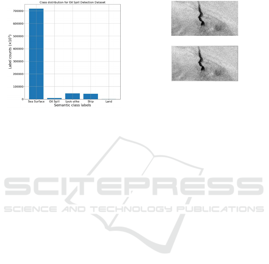
Figure 1: Plot showing the distribution of the semantic

classes in the Oil Spill Detection Dataset.

bers the other labeled semantic classes in the dataset.

The class of interest in this particular research is “Oil

Spill”, whose occurrence in the dataset is shallow. In

this research, we attempt to train models optimized

for detecting this class. The images in the dataset

are 1250 × 650 in W × H, where W and H represent

the width and height of the image, respectively. In

the work of this article, the training dataset (1002 im-

ages), provided by default, was further split randomly

into 95% (951 images) and 5% (51 images) for —

training and validation sets, respectively. This was

done to perform a 5-fold cross-validation with ran-

domized validation sets.

3.2 Image Preprocessing & Data

Augmentation

In their research, Marios Krestenitis et al. used

smaller image patches to train various models

(Krestenitis et al., 2019). The smallest and largest im-

age patch sizes used in their research were 320 × 320

and 336 × 336, respectively. In the work of this ar-

ticle, the original images, in 1250 × 650 dimensions,

are padded with patches on all the 4 sides of the image

to produce resulting images of 1280 × 672. An orig-

inal sample image from the training set and its corre-

sponding padded image are shown in Figures 2(a) and

2(b), respectively. So, higher resolution images are

used as input to the models, compared to those used

by Marios Krestenitis et al. (Krestenitis et al., 2019).

The patch padding is done in such a way as to select

a patch of pixels with the sea surface. A random sam-

ple image from the training set is selected to make

this patching task more straightforward. Data aug-

mentation is applied to increase the size of the train-

(a)

(b)

Figure 2: (a) Example of an original image from the training

set. (b) A sample padded image from the training set.

ing dataset. Random horizontal and vertical ﬂips are

applied only on the training set for data augmentation.

The images are normalized using the mean and stan-

dard deviation of the training set. Then, the normal-

ized images are used as input for the various models

used in this research.

3.3 Models

3.3.1 Residual Networks

Increasing the depth of the convolutional neural net-

works (CNNs) beyond a certain point adversely af-

fected the model’s accuracy due to the vanishing and

exploding gradient problems. To solve this, Residual

Network (ResNet) (He et al., 2015) was introduced

by Kaiming He et al. The ResNet consists of resid-

ual blocks that can learn identity mappings in case of

deeper networks where gradients can vanish. When

stacked, these residual blocks help mitigate the van-

ishing gradient problem by learning an identity func-

tion. Let us consider input x, and the desired mapping

from input to output is denoted by H(x). The residual

denoted by F(x) between the output H(x) and input x

can be computed using the equation (1)

F(x) = H(x) − x (1)

Hence, instead of using the original mapping, it can

be recast into residual mapping using the equation (2)

H(x) = F(x) + x (2)

To perform the above mapping, a constraint is that

F(x) and x should be of the exact dimensions. But

if that is not the case, then one can use a projection

vector W

to match the dimensions. This is shown in

equation (3).

y = F(x, {W

}) +W

x (3)

Oil Spill Segmentation Using Deep Encoder-Decoder Models

743

Kaiming He et al. (He et al., 2015) showed that it was

easier to learn the residual mapping than the original

mapping. In this article, various pre-trained variants

of ResNet models — ResNet-18, ResNet-34, ResNet-

50, and ResNet-101 encoders are used, i.e., without

the ﬁnal classiﬁcation layer that was used for ob-

ject recognition on the ImageNet dataset (Deng et al.,

2009; Russakovsky et al., 2015; He et al., 2015).

3.3.2 EfﬁcientNet

Neural Architecture Search (NAS) was proposed to

optimize network architecture for image classiﬁca-

tion by Zoph et al. (Zoph et al., 2017). The train-

ing bottlenecks of EfﬁcientNet were addressed, and

EfﬁcientNetV2 was proposed by Mingxing Tan et al.

(Tan et al., 2019; Tan and Le, 2021). The main

change was replacing the MBConv block of Efﬁcient-

Net with a new block proposed by Mingxing Tan et

al., the FusedMBConv block, in the early layers. In

the MBConv block, a 3 × 3 depthwise convolution

layer was followed by a 1 × 1 normal convolution

layer. This was replaced in the FusedMBConv block

with a single fused 3 × 3 convolution layer. The other

changes in EfﬁcientNetV2 were to use 3 × 3 kernel

sizes instead of larger kernel sizes but with more lay-

ers and a smaller expansion ratio for MBConv blocks

since smaller expansion ratios and removal of the last

stride-1 stage, which were optimizations towards a re-

duction of the memory access overhead (Tan and Le,

2021).

3.3.3 DeepLabV3 & DeepLabV3+

The output of the encoder was provided as the input

to the decoder, i.e., one of the decoders considered in

this research — DeepLabV3 and DeepLabV3+. In the

DeepLabV3 decoder, Atrous Spatial Pyramid Pool-

ing (ASPP) block was used (Chen et al., 2017; Chen

et al., 2016). This was a modiﬁcation of earlier ver-

sions of the DeepLab decoder where atrous convo-

lution layers were used instead of standard convolu-

tion layers. A dilation rate is used in atrous or di-

lated convolution, which uses a larger view of pix-

els when the kernel is applied to the image. In this

ASPP block, there were four atrous convolution lay-

ers. ASPP has an average pooling layer applied on

the feature maps from the encoder block to provide

global context information. The outputs of all these

ﬁve layers of the ASPP block were concatenated, and

bilinear upsampling was applied to produce feature

maps with the exact dimensions of the input image

dimensions. There were some minor changes to the

DeepLabV3+ decoder when compared with that of

DeepLabV2 (Chen et al., 2017; Chen et al., 2018).

The outputs of all ﬁve layers of the ASPP block were

concatenated, and bilinear upsampling by a factor of

4 was applied. To the corresponding features from

the encoder block, a 1 × 1 convolution was used to

balance the importance between the backbone’s low-

level features and the encoder block’s compressed se-

mantic features. The resulting features were concate-

nated with upsampled features followed by 3 convo-

lution layers to reﬁne the concatenated features. This

connection from the encoder block and concatenation

was a minor change in the DeepLabV3+ decoder. The

resulting feature maps were upsampled using bilinear

upsampling to produce feature maps with the exact

dimensions of the input image dimensions.

3.4 Training Models

The following encoders are used in this research —

ResNet-18, ResNet-34, ResNet-50, ResNet-101, Efﬁ-

cientNetV2S, and EfﬁcientNetV2M (He et al., 2015;

Tan and Le, 2021). The pre-trained models trained on

the ImageNet dataset are used for the encoder mod-

els using transfer learning (Bengio, 2012; Deng et al.,

2009; Russakovsky et al., 2015). The following de-

coders are used in this research — DeepLabV3 and

DeepLabV3+ (Chen et al., 2017; Chen et al., 2018).

All the encoder-decoder models are trained end to end

for 100 epochs, and the hyperparameters are obtained

empirically. Mean categorical cross-entropy loss is

used since the dataset contained 5 semantic classes.

The categorical cross-entropy is given by Euqation 4

where c

denotes the encoded class and p

denotes the

probability of the class as predicted by the model for

every one of the n classes in the dataset. The Stochas-

tic Gradient Descent (SGD) optimizer is used with an

initial learning rate of 1 × 10

−2

, a momentum of 0.9,

and a weight decay of 1 × 10

−4

. Liang-Chieh Chen

et al. observed that the performance of the segmen-

tation model was higher when SGD was combined

with the Polynomial learning rate scheduler (Chen

et al., 2016). In this research, the SGD optimizer

is combined with a polynomial learning rate sched-

uler, where the learning rate decays in a polynomial

fashion. The Polynomial learning rate scheduler is

given by 5 where lr

is the initial learning rate, e is

the current epoch, T

is the total number of epochs,

and power controls the learning rate decay. Learning

may be hampered once the learning rate at any epoch

goes below a certain threshold and becomes closer to

zero. To avoid this, a minimum learning rate is used

as a threshold, and if the learning rate goes below the

threshold, the threshold learning rate is used. For the

Polynomial learning rate scheduler, the parameters —

is set to 1 ×10

−2

, power is set to 0.9 and the min-

ICPRAM 2025 - 14th International Conference on Pattern Recognition Applications and Methods

744

Table 1: Batch sizes of different models used for training.

Encoder Decoder #Params Batch

(millions) size

ResNet-18 DeepLabV3+ 12.34 32

ResNet-34 DeepLabV3+ 22.45 24

ResNet-50 DeepLabV3+ 25.07 8

ResNet-101 DeepLabV3+ 44.06 8

EfﬁcientNetV2S DeepLabV3 21.42 8

EfﬁcientNetV2M DeepLabV3 54.11 4

imum learning rate is set to 1 × 10

−6

CE(c, p) = −

∑

i=1

log(p

) (4)

lr = lr

× (1 −

)

power

(5)

A weight decay is used for regularization in the SGD

optimizer, a dropout layer with a dropout rate of 10%,

and data augmentation with horizontal and vertical

ﬂips is used. Different batch sizes are used to train

different models as they differ in the number of pa-

rameters that require different amounts of Graphical

Processing Unit (GPU) memory. Table 1 shows the

batch size used to train different models. The Nvidia

V100 GPU available on the high-performance com-

puting cluster is used to train the models.

3.5 Transfer Learning

Transfer learning is a machine learning approach that

simpliﬁes the training of deep neural networks from

scratch (Bengio, 2012). Transfer learning allows us

to use a previously developed machine learning model

for a new but related task. This approach has gained

signiﬁcant popularity in the ﬁeld of computer vision,

primarily due to the impressive capability of CNNs to

adapt learned low-level feature extraction for various

tasks.

3.6 Evaluation Metrics

For evaluation of the performance of the models, In-

tersection over Union (IoU) is used (Krestenitis et al.,

2019). The mean IoU (m-IoU) is the mean of the IoU

of the different semantic classes in the dataset. The

class IoU is the IoU computed for a semantic class

individually.

4 RESULTS & DISCUSSION

4.1 Quantitative Analysis

A 5-fold cross-validation was performed to ﬁnd the

deviation of the performance of the models on differ-

Table 2: Performance metrics of various models for a 5-fold

validation on the randomized validation sets.

Encoder Decoder m-IoU (%)

ResNet-18 DeepLabV3+ 67.345 ± 1.407

ResNet-34 DeepLabV3+ 67.522 ± 3.898

ResNet-50 DeepLabV3+ 67.578 ± 3.631

ResNet-101 DeepLabV3+ 68.152 ± 2.470

EfﬁcientNetV2S DeepLabV3 60.668 ± 2.796

EfﬁcientNetV2M DeepLabV3 58.997± 3.021

ent random validation splits. Table 2 shows the per-

formance metrics of the various models for a 5-fold

validation on the randomized validation sets. For all

the models, there is a signiﬁcant deviation of m-IoU

(greater than 1%) across the 5-fold validation. This is

expected since the dataset was highly imbalanced and

was split randomly into training and validation sets.

Some splits would have higher m-IoU than others, de-

pending on the division of the samples and their dis-

tribution of semantic classes. Hence, the m-IoU of the

validation set depends on the split in cross-validation

experiments.

Table 3 shows the performance metrics of the best-

performing model for each of the models on the test

set with 110 images. The best m-IoU on the test set

was 64.868% for the model with the ResNet-50 en-

coder and DeepLabV3+ decoder. This model’s per-

formance is slightly lower than the best-performing

model from the previous research by Mario Kresteni-

tis et al., which scored m-IoU of 65.06% on the test

set (Krestenitis et al., 2019). Table 1 also shows the

number of parameters in various models. If the model

with EfﬁcientNetV2M encoder and DeepLabV3 de-

coder with 54.11 million parameters and the model

with ResNet-50 encoder and DeepLabV3+ decoder

with just 25.07 million parameters are considered,

their performances are 55.504% and 64.868% respec-

tively. This shows that increasing the number of pa-

rameters in a model would not necessarily improve

the model’s performance for every task.

Table 3: Performance metrics of the best-performing model

for each model on the test set with 110 images.

Encoder Decoder m-IoU (%)

ResNet-18 DeepLabV3+ 59.647

ResNet-34 DeepLabV3+ 60.843

ResNet-50 DeepLabV3+ 64.868

ResNet-101 DeepLabV3+ 64.677

EfﬁcientNetV2S DeepLabV3 55.492

EfﬁcientNetV2M DeepLabV3 55.504

Table 4 shows the classwise performance metrics

of the best-performing models on the test set with 110

Oil Spill Segmentation Using Deep Encoder-Decoder Models

745

images, i.e., the model with ResNet-50 encoder and

DeepLabV3+ decoder from this research and best-

performing model from Marios Krestenitis et al. re-

search. Marios et al. best model scored a class IoU of

53.38% and 55.40% for the “oil spill” and “oil spill

look-alike” classes, respectively (Krestenitis et al.,

2019). On the other hand, the best-performing model

from this research scored a class IoU of 61.549%

and 40.773% for the “oil spill” and “oil spill look-

alike” classes, respectively. Although the model from

this research scored lower for the “oil spill look-

alike” class, it still scored higher for the “oil spill”

class, which is of more interest. Another observa-

tion is that the performance of detection of “ship”

is more remarkable for the best-performing model

from this research when compared with that of the

best-performing model from Marios Krestenitis et al.,

with class IoU of 33.378% and 27.63% respectively.

For the remaining classes, i.e., the “sea surface” and

“land”, the performances of the best-performing mod-

els from this research and Marios Krestenitis et al. are

comparable.

Table 4: Classwise performance metrics, i.e., the class IoU

of the best-performing model on the test set with 110 im-

ages.

Class IoU (%)

Our best Best model of

model Marios et al.

Semantic Class

Sea surface 96.422 96.43

Oil spill 61.549 53.38

Oil spill look-alike 40.773 55.40

Ship 33.378 27.63

Land 92.218 92.44

mean 64.868 65.06

4.2 Qualitative Analysis

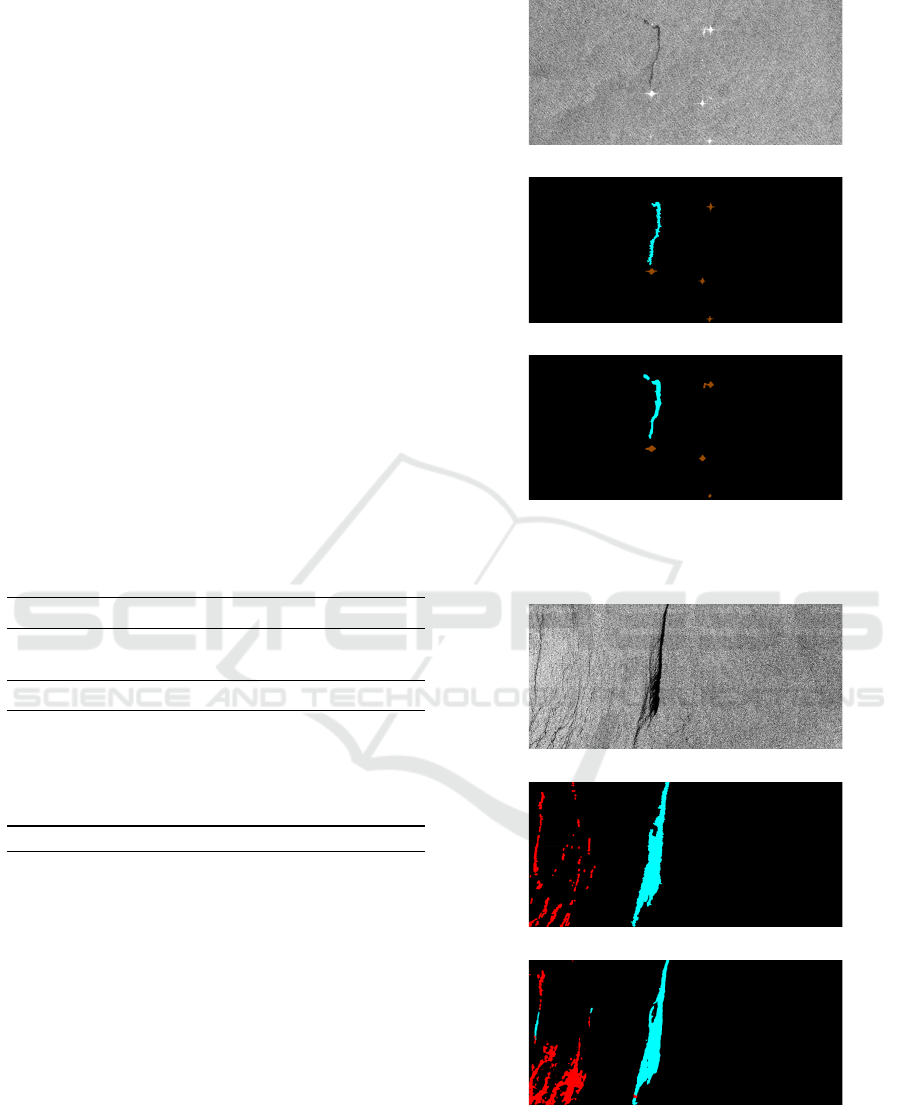
From the test sample shown in Figure 3(a), its ground-

truth mask shown in Figure 3(b) and its prediction

mask shown in Figure 3(c), it can be observed that

relatively smaller areas of “oil spills” (in Cyan) along

with “ships” (in Brown) are detected by the model

with reasonable accuracy, for this sample. From Fig-

ures 4(a), 4(b), and 4(c), it can be observed that rel-

atively more signiﬁcant areas of “oil spills” are de-

tected by the model with reasonable accuracy. In this

test sample, the model confuses the classes ”oil spill”

and ”oil spill look-alike,” resulting in portions of the

regions being predicted for both classes. However,

from Figures 5(a), 5(b), and 5(c), it can be observed

that relatively more signiﬁcant areas of “oil spills” are

(a)

(b)

(c)

Figure 3: (a) Sample test image (b) Groundtruth (c) Pre-

dicted mask.

(a)

(b)

(c)

Figure 4: (a) Sample test image (b) Groundtruth (c) Pre-

dicted mask.

not detected by the model with reasonable accuracy.

The model showcases a range of detections, including

ICPRAM 2025 - 14th International Conference on Pattern Recognition Applications and Methods

746

(a)

(b)

(c)

Figure 5: (a) Sample test image (b) Groundtruth (c) Pre-

dicted mask.

highly accurate results as well as some less reliable

ones.

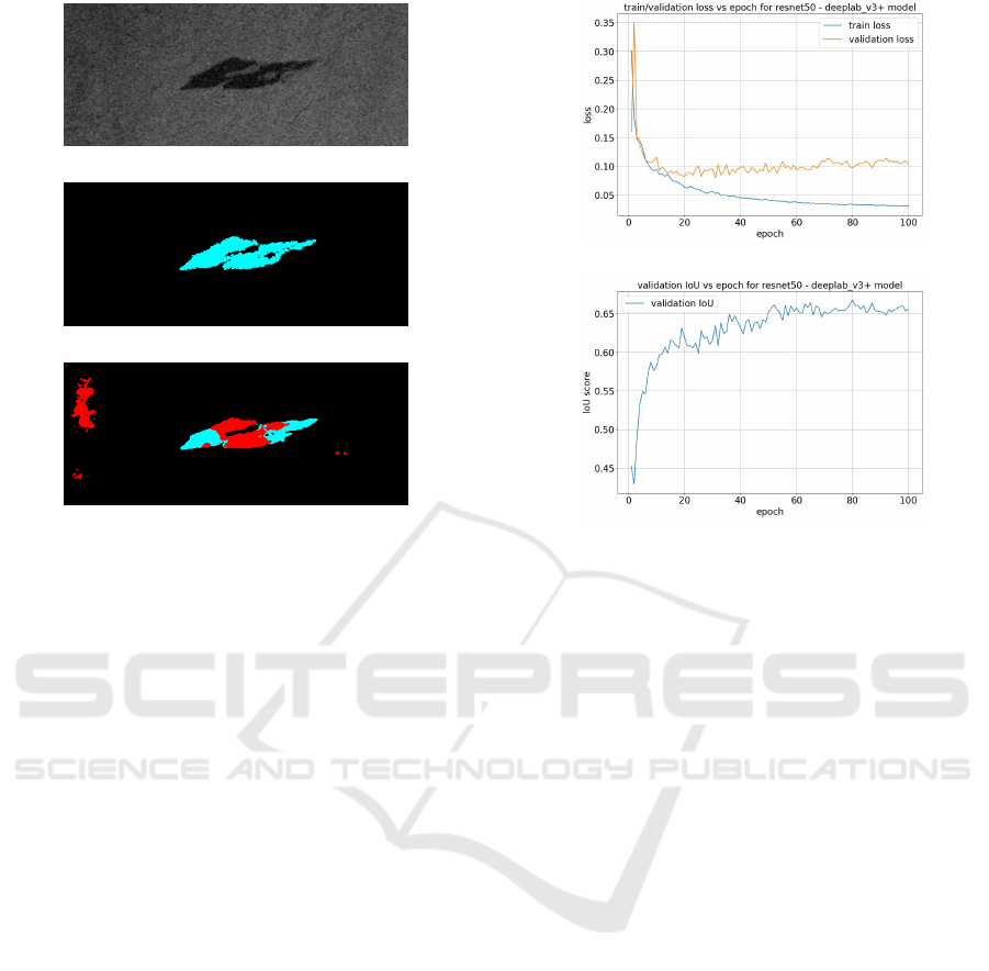
4.3 Learning Curves

Figure 6(a) shows the plot of losses for training

and validation sets vs. epoch for the model with

ResNet-50 encoder and DeepLabV3+ decoder, i.e.,

for the best-performing models from our experiments.

6(b) shows the plot of m-IoU for validation set vs.

epoch for the model with ResNet-50 encoder and

DeepLabV3+ decoder. The two learning curve ﬁg-

ures show that the validation metrics converge, i.e.,

they do not deviate much after considerable learning.

However, some overﬁtting occurs as the gap between

the training and validation losses widens with an in-

crease in the number of epochs.

5 CONCLUSIONS

In the earlier research on the same topic and dataset,

high-dimensional images were divided into smaller

patches that served as input for the models. The best-

performing model achieved a mean Intersection over

Union (m-IoU) of 65.06% and a class IoU of 53.38%.

In contrast, this article utilized high-dimensional im-

ages as direct input to the model without partition-

ing them into patches. The best-performing model

in this study, which employed a ResNet-50 encoder

(a)

(b)

Figure 6: (a) Plot of training and validation losses for the

model with ResNet-50 encoder and DeepLabV3+ decoder.

(b) Plot of validation m-IoU for the model with ResNet-50

encoder and DeepLabV3+ decoder.

and a DeepLabV3+ decoder, achieved an m-IoU of

64.868% and a class IoU of 61.549% for the ”oil

spill” class. This represents a new benchmark result,

indicating that using high-dimensional images can en-

hance the performance of ”oil spill” detection. How-

ever, the dataset also contains samples from the ”oil

spill look-alike” class, which can create confusion for

the trained models, making it challenging to distin-

guish between the ”oil spill” and ”oil spill look-alike”

classes. There is potential for further experimentation

with various encoders and decoders to achieve bet-

ter results. Additionally, the current encoders and de-

coders used in this research could be improved by in-

corporating visual self-attention modules. These en-

hancements can be explored in future research follow-

ing the analysis presented in this article.

ACKNOWLEDGEMENTS

We thank the Center for Information Technology of

the University of Groningen for their support and for

providing access to the Peregrine high-performance

computing cluster. We also thank Marios Krestenitis

and Konstantinos Ioannidis for creating and providing

the dataset.

Oil Spill Segmentation Using Deep Encoder-Decoder Models

747

REFERENCES

Bengio, Y. (2012). Deep learning of representations for

unsupervised and transfer learning. In Guyon, I.,

Dror, G., Lemaire, V., Taylor, G., and Silver, D., edi-

tors, Proceedings of ICML Workshop on Unsupervised

and Transfer Learning, volume 27 of Proceedings of

Machine Learning Research, pages 17–36, Bellevue,

Washington, USA. PMLR.

Broekema, W. (2016). Crisis-induced learning and issue

politicization in the eu: The braer, sea empress, erika,

and prestige oil spill disasters. Public Administration,

94(2):381–398.

Chaurasia, A. and Culurciello, E. (2017). Linknet: Exploit-

ing encoder representations for efﬁcient semantic seg-

mentation. CoRR, abs/1707.03718.

Chen, L., Papandreou, G., Kokkinos, I., Murphy, K.,

and Yuille, A. L. (2016). Deeplab: Semantic

image segmentation with deep convolutional nets,

atrous convolution, and fully connected crfs. CoRR,

abs/1606.00915.

Chen, L., Papandreou, G., Schroff, F., and Adam, H.

(2017). Rethinking atrous convolution for semantic

image segmentation. CoRR, abs/1706.05587.

Chen, L., Zhu, Y., Papandreou, G., Schroff, F., and Adam,

H. (2018). Encoder-decoder with atrous separable

convolution for semantic image segmentation. CoRR,

abs/1802.02611.

Cordts, M., Omran, M., Ramos, S., Rehfeld, T., Enzweiler,

M., Benenson, R., Franke, U., Roth, S., and Schiele,

B. (2016). The cityscapes dataset for semantic urban

scene understanding. In Proc. of the IEEE Conference

on Computer Vision and Pattern Recognition (CVPR).

Deng, J., Dong, W., Socher, R., Li, L.-J., Li, K., and Fei-

Fei, L. (2009). ImageNet: A Large-Scale Hierarchical

Image Database. In CVPR09.

Deng, L. (2012). The mnist database of handwritten digit

images for machine learning research [best of the

web]. IEEE Signal Processing Magazine, 29(6):141–

142.

Dunnet, G. M., Crisp, D. J., Conan, G., Bournaud, R.,

Cole, H. A., and Clark, R. (1982). Oil pollution and

seabird populations. Philosophical Transactions of

the Royal Society of London. B, Biological Sciences,

297(1087):413–427.

He, K., Zhang, X., Ren, S., and Sun, J. (2015). Deep

residual learning for image recognition. CoRR,

abs/1512.03385.

Krestenitis, M., Orfanidis, G. A., Ioannidis, K., Avgeri-

nakis, K., Vrochidis, S., and Kompatsiaris, Y. (2019).

Oil spill identiﬁcation from satellite images using

deep neural networks. Remote. Sens., 11:1762.

Krizhevsky, A., Sutskever, I., and Hinton, G. E. (2012).

Imagenet classiﬁcation with deep convolutional neu-

ral networks. In Pereira, F., Burges, C., Bottou, L.,

and Weinberger, K., editors, Advances in Neural In-

formation Processing Systems, volume 25. Curran As-

sociates, Inc.

LeCun, Y., Boser, B., Denker, J. S., Henderson, D., Howard,

R. E., Hubbard, W., and Jackel, L. D. (1989). Back-

propagation applied to handwritten zip code recogni-

tion. Neural Computation, 1(4):541–551.

LeCun, Y., Bottou, L., Bengio, Y., and Haffner, P. (1998).

Gradient-based learning applied to document recogni-

tion. Proceedings of the IEEE, 86(11):2278–2324.

Lin, T., Maire, M., Belongie, S. J., Bourdev, L. D., Girshick,

R. B., Hays, J., Perona, P., Ramanan, D., Doll

ar, P.,

and Zitnick, C. L. (2014). Microsoft COCO: common

objects in context. CoRR, abs/1405.0312.

Long, J., Shelhamer, E., and Darrell, T. (2014). Fully

convolutional networks for semantic segmentation.

CoRR, abs/1411.4038.

Middlebrook, A., Ahmadov, R., Atlas, E., Bahreini, R.,

Blake, D., Brioude, J., Brock, C., de Gouw, J., Fahey,

D., Fehsenfeld, F., Holloway, J., Lueb, R., McKeen,

S., Meagher, J., Meinardi, S., Murphy, D., Parrish, D.,

Peischl, J., and Watts, L. (2010). Air quality impact

of the deepwater horizon oil spill (invited). AGU Fall

Meeting Abstracts, pages 02–.

Ronneberger, O., Fischer, P., and Brox, T. (2015). U-net:

Convolutional networks for biomedical image seg-

mentation. CoRR, abs/1505.04597.

Russakovsky, O., Deng, J., Su, H., Krause, J., Satheesh,

S., Ma, S., Huang, Z., Karpathy, A., Khosla, A.,

Bernstein, M., Berg, A. C., and Fei-Fei, L. (2015).

ImageNet Large Scale Visual Recognition Challenge.

International Journal of Computer Vision (IJCV),

115(3):211–252.

Sandler, M., Howard, A. G., Zhu, M., Zhmoginov, A., and

Chen, L. (2018). Inverted residuals and linear bottle-

necks: Mobile networks for classiﬁcation, detection

and segmentation. CoRR, abs/1801.04381.

Shigenaka, G. (2009). Hindsight and foresight: 20 years

after the exxon valdez spill. USA: National Oceanic

and Atmospheric Administration, page 18.

Tan, M. and Le, Q. V. (2021). Efﬁcientnetv2: Smaller mod-

els and faster training. CoRR, abs/2104.00298.

Tan, M., Pang, R., and Le, Q. V. (2019). Efﬁcient-

det: Scalable and efﬁcient object detection. CoRR,

abs/1911.09070.

Zhao, H., Shi, J., Qi, X., Wang, X., and Jia, J. (2016). Pyra-

mid scene parsing network. CoRR, abs/1612.01105.

Zoph, B., Vasudevan, V., Shlens, J., and Le, Q. V. (2017).

Learning transferable architectures for scalable image

recognition. CoRR, abs/1707.07012.

ICPRAM 2025 - 14th International Conference on Pattern Recognition Applications and Methods

748