CGLearn: Consistent Gradient-Based Learning for Out-of-Distribution

Generalization

Jawad Chowdhury

and Gabriel Terejanu

Department of Computer Science, University of North Carolina at Charlotte, North Carolina, U.S.A.

Keywords:

Invariant Learning, Causal Invariance, Robust Machine Learning, Domain Generalization, Supervised Deep

Learning, Optimization for Neural Networks.

Abstract:

Improving generalization and achieving highly predictive, robust machine learning models necessitates learn-

ing the underlying causal structure of the variables of interest. A prominent and effective method for this is

learning invariant predictors across multiple environments. In this work, we introduce a simple yet powerful

approach, CGLearn, which relies on the agreement of gradients across various environments. This agreement

serves as a powerful indication of reliable features, while disagreement suggests less reliability due to poten-

tial differences in underlying causal mechanisms. Our proposed method demonstrates superior performance

compared to state-of-the-art methods in both linear and nonlinear settings across various regression and classi-

ﬁcation tasks. CGLearn shows robust applicability even in the absence of separate environments by exploiting

invariance across different subsamples of observational data. Comprehensive experiments on both synthetic

and real-world datasets highlight its effectiveness in diverse scenarios. Our ﬁndings underscore the impor-

tance of leveraging gradient agreement for learning causal invariance, providing a signiﬁcant step forward in

the ﬁeld of robust machine learning. The source code of the linear and nonlinear implementation of CGLearn

is open-source and available at: https://github.com/hasanjawad001/CGLearn.

1 INTRODUCTION

Machine learning models have achieved remarkable

success in various domains driven by the recent avail-

ability of large datasets, sophisticated algorithms, and

highly advanced complex models. However, these

models perform well only when the test data fol-

lows the same distribution as the training data (i.i.d.),

but they often suffer from overﬁtting due to over-

parametrization, learning spurious correlations from

training data (Sagawa et al., 2020; Wang et al., 2021;

Ming et al., 2022). This issue arises because tradi-

tional models focus on predictive power without con-

sidering the causal relationships underlying the data.

As a result, when the training and test distributions

differ, models that rely on spurious correlations can

perform very poorly, compromising their robustness,

leading to poor generalization on out-of-distribution

(OOD) test data (Arjovsky et al., 2019; He et al.,

2021).

Learning causal relationships is the key to model

https://orcid.org/0009-0004-6986-3063

https://orcid.org/0000-0002-8934-9836

explainability and enhancing generalization and ro-

bustness (Shin, 2021; Wang et al., 2022; Santil-

lan, 2023). Although the ideal method for learn-

ing causal structures is through Randomized Control

Trials (RCTs), these are often expensive, unethical,

or impractical. Various methods have been devel-

oped for causal discovery. Constraint-based meth-

ods use conditional independence tests to identify

causal directions (Spirtes et al., 2001; Pearl, 2009;

Colombo et al., 2012). This however often results in

the Markov Equivalence Class (MEC) of causal struc-

tures. Score-based methods optimize causal graphs

over Directed Acyclic Graphs (DAGs) (Chickering,

2002; Ramsey et al., 2017; Huang et al., 2018),

but the combinatorial nature of the search space can

make it computationally expensive. Advances like

NOTEARS (Zheng et al., 2018) transform this combi-

natorial challenge into continuous optimization, lead-

ing to various effective variants (Zheng et al., 2020;

Yu et al., 2019; Lachapelle et al., 2019; Wei et al.,

2020; Ng et al., 2020; Ng et al., 2022). How-

ever, learning causal structures purely from observa-

tional data can be challenging due to issues like se-

lection bias, measurement errors, and confounding

Chowdhury, J. and Terejanu, G.

CGLearn: Consistent Gradient-Based Learning for Out-of-Distribution Generalization.

DOI: 10.5220/0013260400003905

Paper published under CC license (CC BY-NC-ND 4.0)

In Proceedings of the 14th International Conference on Pattern Recognition Applications and Methods (ICPRAM 2025), pages 103-112

ISBN: 978-989-758-730-6; ISSN: 2184-4313

103

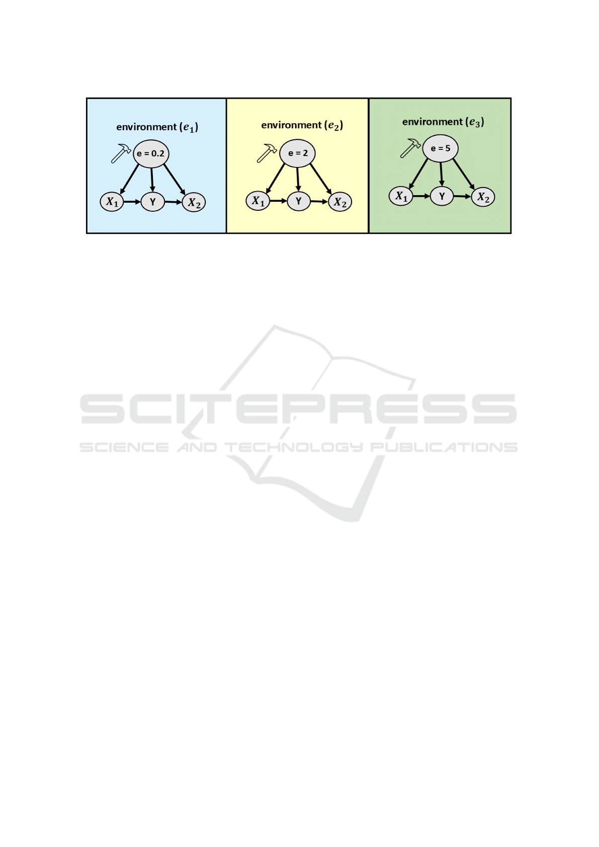
Figure 1: Illustration of three environments generated by intervening on the variable e, which takes distinct values e = 0.2,

e = 2, and e = 5 in environments e

, e

, and e

, respectively. In each environment, X

acts as a causal factor for the target

variable Y , while X

is a spurious (non-causal) factor with respect to Y . This ﬁgure exempliﬁes how different interventions on

e create distinct environments.

factors (Zadrozny, 2004; Torralba and Efros, 2011).

Moreover, relying solely on empirical risk optimiza-

tion can result in models highly dependent on spuri-

ous relationships. To tackle this problem, researchers

often use prior domain knowledge to improve causal

discovery (O’Donnell et al., 2006; Gencoglu and Gru-

ber, 2020; Andrews et al., 2020; Liu et al., 2021;

Chowdhury. et al., 2023; Chowdhury and Terejanu,

2023). Unfortunately, many causal discovery meth-

ods depend on speciﬁc assumptions (e.g., linearity,

non-Gaussian noise) that do not always hold in real-

world data. In addition to that some of these methods

exploit variance scales e.g. var-sortability to identify

causal orderings, performing well on unstandardized

data but poorly after standardization (Reisach et al.,

2021; Kaiser and Sipos, 2022; Reisach et al., 2024;

Ormaniec et al., 2024).

A recent line of study focuses on exploiting the

invariance property of causal relationships across dif-

ferent environments. Methods like Invariant Causal

Prediction (ICP) (Peters et al., 2016) aim to identify

causal predictors by ensuring the conditional distri-

bution of the target given these predictors remains

stable across environments. This method leverages

the invariance of causal relationships under differ-

ent interventions, iterating over feature subsets to

ﬁnd those invariant across environments, considering

them as potential causal parents of the target vari-

able. Another study, IRM (Arjovsky et al., 2019)

optimizes a penalty function to achieve OOD gener-

alization for predictive models, ensuring robust per-

formance across environments. These methods sig-

niﬁcantly reduce the absorption of spurious correla-

tions by focusing on stable and invariant relation-

ships. The invariant learning framework provides a

promising approach to improve model robustness and

generalization in the presence of distribution shifts,

with various domains exploiting invariance to learn

better predictors and robust models (Montavon et al.,

2012; Wang et al., 2017; Chowdhury et al., 2024;

Bose and Roy, 2024). Some relevant works such as

AND-mask (Parascandolo et al., 2020), Fishr (Rame

et al., 2022), Fish (Shi et al., 2021), IGA (Koyama

and Yamaguchi, 2020) use environment-speciﬁc gra-

dients to improve generalization in diverse settings.

Moreover, approaches examining the signal-to-noise

ratio (GSNR) in gradients, such as the work in Ref.

study (Liu et al., 2020), measure the alignment of gra-

dient directions across samples, while a similar strat-

egy has been employed in large-batch training scenar-

ios to improve model stability (Jiang et al., 2023).

Motivated by this line of work and the current

drawbacks of existing methods in structure learning

and OOD generalization, we introduce CGLearn, a

general framework designed to improve the gener-

alization of machine learning models by leveraging

gradient consistency across different environments.

CGLearn does not require extensive domain knowl-

edge or assumptions over data linearity or noise, mak-

ing it a versatile and practical approach for learning

robust predictive models. By focusing on feature in-

variance, emphasizing on reliable features, and reduc-

ing dependence on spurious correlations, CGLearn

enhances the reliability and robustness of the mod-

els. The main contributions of this study are stated as

follows:

• We propose a novel general framework, CGLearn,

which improves consistency in learning robust

predictors by focusing on features that show con-

sistent behavior across environments.

• We provide both linear and nonlinear implemen-

tations of CGLearn, demonstrating its versatility

and applicability across different model architec-

tures.

• We demonstrate that CGLearn achieves superior

ICPRAM 2025 - 14th International Conference on Pattern Recognition Applications and Methods

104

predictive power and generalization, even without

multiple environments, unlike most state-of-the-

art methods in this arena that require diverse envi-

ronments for effective generalization.

• Our empirical evaluations on synthetic and real-

world datasets, covering both linear and nonlinear

settings, as well as regression and classiﬁcation

tasks, validate the effectiveness and robustness of

the proposed method.

The remainder of this paper is organized as fol-

lows: First, we delve into the methodology of

CGLearn, detailing its linear and nonlinear imple-

mentations. Next, we present our experimental set-

tings and evaluations. Finally, we encapsulate our

conclusions, highlight the signiﬁcant takeaways, and

discuss future directions.

2 METHODOLOGY

In this section, we present the methodology of

CGLearn, detailing both its linear and nonlinear im-

plementations. We start by explaining the regular Em-

pirical Risk Minimization (ERM) approach and then

introduce the concept of gradient consistency used in

CGLearn. The primary concept of CGLearn is to en-

force gradient consistency for each factor of our vari-

able of interest across multiple environments to iden-

tify and utilize invariant features, thereby enhancing

generalization and reducing dependence on spurious

correlations.

2.1 Empirical Risk Minimization

(ERM)

Let’s consider a simple linear problem where the goal

is to predict the target variable Y using two features

(causal) and X

(spurious) across multiple envi-

ronments. Let e

, e

, . . . , e

represent different envi-

ronments. Environments can be considered as distinct

distributions generated by different interventions, all

of which share similar underlying causal mechanisms

(see Figure. 1).

In the ERM framework, the weights for the fea-

tures are updated by minimizing the empirical risk

or the cost function (L), which is typically the mean

squared error (MSE) between the predicted and actual

values for a regression problem and cross-entropy loss

for a classiﬁcation task. Suppose the weights for the

features at step t are w

for X

and w

for X

. The

gradient of the loss (L) with respect to the weight as-

sociated with the j-th feature X

in environment e

given by ∇L

, where j ∈ {1, 2} and i ∈ {1, . . . , m}.

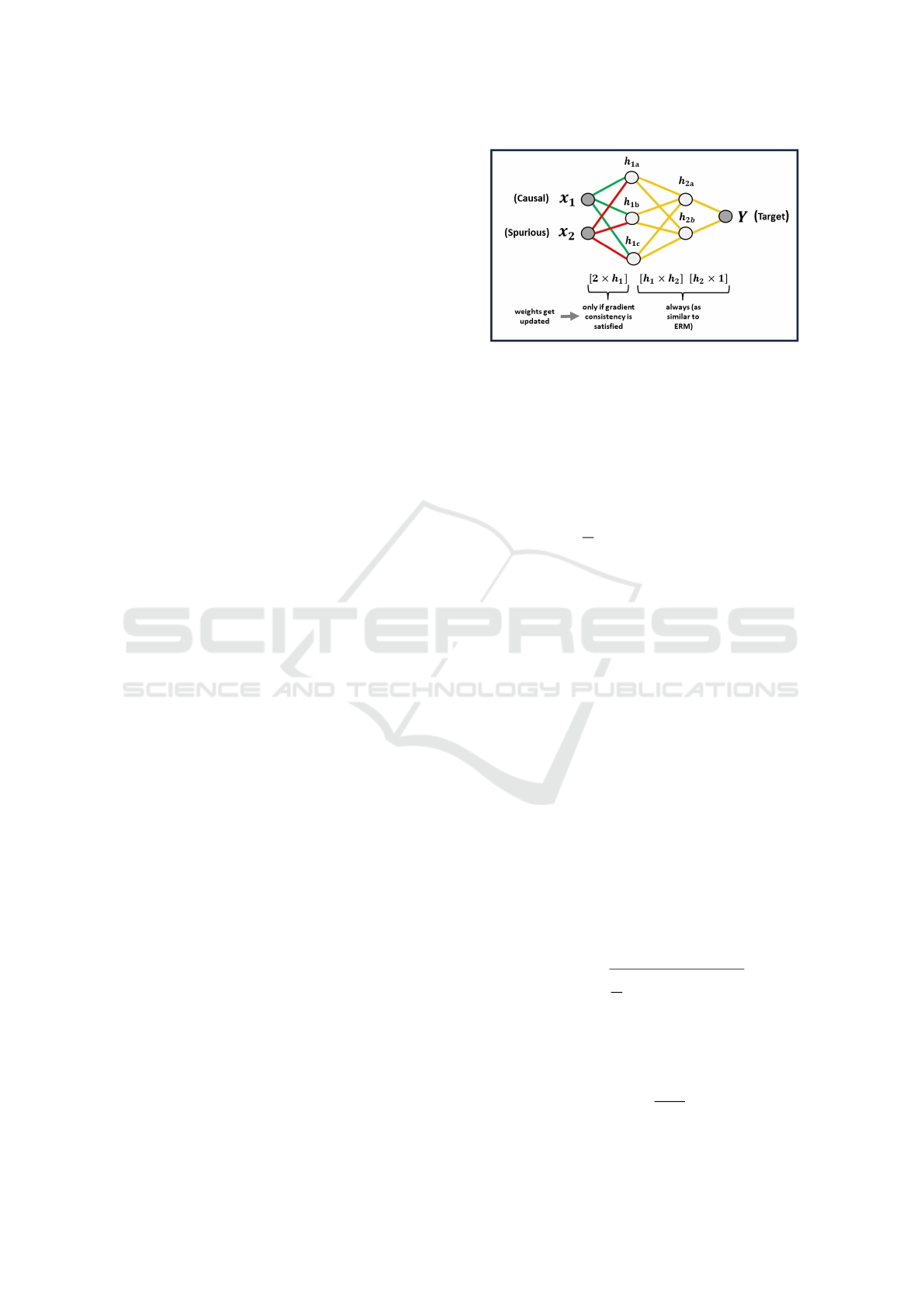
Figure 2: Nonlinear MLP implementation of CGLearn. X

(causal) and X

(spurious) feed into the ﬁrst hidden layer h

Weight updates in h

are performed based on gradient con-

sistency (using L

-norm) for each feature across all training

environments. The rest of the weights such as weights in h

are updated similarly to ERM (without imposing any con-

sistency constraints).

The aggregated gradient across all environments

can be calculated as the mean of the gradients:

grad

∑

i=1

∇L

for j ∈ {1, 2} (1)

Using this aggregated gradient, the weights are

updated as follows:

t+1

= w

− ηµ

grad

for j ∈ {1, 2} (2)

where η is the learning rate. In this setup of a standard

Empirical Risk Minimization, the weights for both X

and X

get updated in each step regardless of their

consistency across environments.

2.2 Linear Implementation of CGLearn

CGLearn modiﬁes this approach by introducing a

consistency check for the gradients. The idea is to

update the weights only if the gradients are consistent

across the available environments. This strategy fo-

cuses on invariant features and ignores spurious ones,

expecting better generalization.

First, we calculate the gradient of each feature in

every environment, as described in the previous sec-

tion. The mean of the gradients can be calculated as

described in Eq. 1. Next, we compute the standard

deviation of the gradients for each feature across all

environments as follows:

grad

∑

i=1



∇L

− µ

grad



(3)

We then calculate the consistency ratio, which is

the absolute value of the ratio of the mean gradient to

the standard deviation of the gradients:

ratio



grad



(4)

CGLearn: Consistent Gradient-Based Learning for Out-of-Distribution Generalization

105

The consistency ratio, C

ratio

deﬁned in Eq. 4, is

considered to be an indicator of the invariance of the

gradient of variable X

across all the training environ-

ments. A relatively larger mean compared to the stan-

dard deviation would indicate more similar or invari-

ant gradients across the environments for the feature

, resulting in a higher value of C

ratio

. On the other

hand, a larger standard deviation indicates more di-

versity across the environments for X

. Finally, we

formulate a consistency mask based on a predeﬁned

threshold C

thresh

mask

(

1 if C

ratio

≥ C

thresh

0 otherwise

(5)

The weights are updated only for the feature that

has a nonzero mask and remains unchanged otherwise

as per the following equation:

t+1

= w

− η



grad

·C

mask



for j ∈ {1, 2} (6)

Considering our motivating example, where X

causal and expected to show more consistency across

environments, C

mask

is expected to be 1. Conversely,

is spurious with respect to the target, expected to

show inconsistency across environments, and C

mask

is expected to be 0. Therefore, the weight for X

mostly updated throughout the training steps while

the weight for X

is not. The model thus focuses

on the features that show consistency for learning the

predictors of the target. This implementation strat-

egy ensures to emphasis on reliable, invariant features

while minimizing the impact of unreliable features

by keeping their weights unchanged (or keeping the

changes to a minimum). As a result, the contributions

of the spurious features remain constant in the context

of the model updates. In the next section, we extend

the CGLearn method to a nonlinear setting using mul-

tilayer perceptron (MLP) as an instance.

2.3 Nonlinear Implementation

For the nonlinear implementation of CGLearn using a

multilayer perceptron (MLP), we focus on the gradi-

ents in the ﬁrst hidden layer (h

), where feature con-

tributions can be distinctly identiﬁed. By controlling

the contribution of spurious features at the ﬁrst hidden

layer, we ensure they do not inﬂuence the ﬁnal output.

The process involves calculating the L

-norm of the

gradients for each feature in each environment, fol-

lowed by determining the consistency ratio and mask

to impose the consistency constraint.

∥∇L

∥

denotes the L

-norm of the gradients of

the j-th feature X

in the i-th environment e

at the ﬁrst

hidden layer h

. We compute the mean and standard

deviation of the L

-norm of the gradients across all

environments as follows:

grad

∑

i=1

∥∇L

∥

(7)

grad

∑

i=1



∥∇L

∥

− µ

grad



(8)

We then calculate the consistency ratio, C

ratio

and

the consistency mask, C

mask

for feature X

by follow-

ing Eq. 4 and 5 respectively. All the weights that

belong to a particular feature, X

in the ﬁrst hidden

layer h

, are updated by following a similar strategy

to Eq. 6. This updating strategy that depends on the

consistency ratio, ensures that only the features that

show consistency across the environments are consid-

ered to be updated. Otherwise, the weights remain un-

changed, effectively treating them as constants similar

to the linear implementation. For weights correspond-

ing to the rest of the model other than the ﬁrst hidden

layer are updated as similar to ERM.

Figure. 2 illustrates a simple demonstration of the

nonlinear MLP implementation of CGLearn. In this

ﬁgure, X

and X

represent causal and spurious fea-

tures, respectively, in accordance with our earlier mo-

tivating example. The gradient consistency is checked

in the ﬁrst hidden layer (h

), and weights are updated

only if the consistency ratio exceeds the threshold, en-

suring that features that show invariance across envi-

ronments are utilized.

In both implementations, the goal is to ensure

that the model relies on features that show invariance

across different environments. This leads to more

robust and generalizable models by reducing depen-

dency on spurious correlations.

3 EXPERIMENTS AND RESULTS

We have considered three different major scenarios

to assess the predictivity, robustness, and generaliza-

tion capabilities of CGLearn. The ﬁrst two scenarios

are the ones where we considered linearly generated

dataset-based experiments and in the last experimen-

tal case we have used the nonlinear implementation

of CGLearn using multilayer perceptron (MLP) and

applied it to different real world regression and clas-

siﬁcation tasks.

For all evaluations, we reported the mean and

standard deviation of the performance metrics consid-

ered. For statistical signiﬁcance tests, we used a t-test

with α = 0.05 as the signiﬁcance level.

ICPRAM 2025 - 14th International Conference on Pattern Recognition Applications and Methods

106

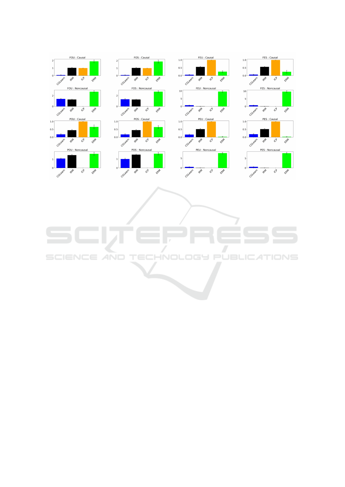
Figure 3: Performance comparison of CGLearn, IRM, ICP, and ERM across various linear multiple environment setups.

Each subplot represents different conﬁgurations of the data, showing the mean squared error (MSE) for causal and noncausal

variables over 50 trials.

3.1 Linear Multiple Environments

To evaluate the performance of our proposed

CGLearn method, we generated synthetic linear

datasets inspired by the approach used in the Invariant

Risk Minimization (IRM) framework (Arjovsky et al.,

2019). Our goal was to create diverse environments to

test the robustness of our model under varying condi-

tions.

We generated eight different experimental setups

based on three key factors. Each setup included

datasets with one target variable Y and ten feature

variables X

to X

. Features X

to X

acted as causal

parents of Y , while X

to X

were inﬂuenced by Y

(non-causal). First, we distinguished between scram-

bled (S) and unscrambled (U) observations by apply-

ing an orthogonal transformation matrix S for scram-

bled data and using the identity matrix I for unscram-

bled data. This scrambling ensures that the features

are not directly aligned with their original scales,

making the learning task more challenging. Second,

we designed fully-observed (F) scenarios where hid-

den confounders did not directly affect the features

(i.e., no hidden confounder effects on features), and

partially-observed (P) scenarios where hidden con-

founders inﬂuenced the features with Gaussian noise.

Third, we incorporated two types of noise for the tar-

get variable Y : homoskedastic (O) noise, where the

noise variance remained constant across different en-

vironments, and heteroskedastic (E) noise, where the

noise variance varied depending on the environment,

increasing with higher values of e. This distinction

captures different real-world scenarios where noise

may or may not depend on external factors. For each

of these eight conﬁgurations (combinations of S/U,

F/P, and O/E), we generated datasets corresponding

to three distinct environments deﬁned by the values

e ∈ {0.2, 2, 5}. Each dataset consisted of 1000 sam-

ples. To ensure consistency with the IRM methodol-

ogy and experimental setup, we used e = 5 as the val-

idation environment and determined the optimal con-

sistency threshold (C

thresh

) for our CGLearn method

using the performance based on this validation data.

We selected the threshold C

thresh

from the candidate

values {0.25, 1, 4, 16, 64} based on validation perfor-

mance. This threshold, which varies based on the pro-

portion of causal and spurious features in the dataset,

is critical for identifying the invariant and most reli-

able features across different environments. For more

details on the data generation process, we refer read-

ers to the IRM paper (Arjovsky et al., 2019).

We compared the performance of CGLearn

with Empirical Risk Minimization (ERM), Invariant

Causal Prediction (ICP) (Peters et al., 2016), and IRM

(Arjovsky et al., 2019). We considered 50 random

trials and reported the results in Figure. 3. In most

cases, our proposed method CGLearn achieves the

lowest mean squared error (MSE), demonstrating su-

perior performance across various test cases to distin-

guish the causal and noncausal factors of the target

by exploiting invariance across environments. IRM

performs better than ERM but does not match the ac-

curacy of CGLearn. ERM shows the highest errors in

most cases, as it fails to differentiate between causal

CGLearn: Consistent Gradient-Based Learning for Out-of-Distribution Generalization

107

and noncausal features, relying on spurious correla-

tions. Interestingly, ICP performs well in noncausal

scenarios but poorly in causal ones. This observa-

tion aligns with the ﬁndings from the IRM study (Ar-

jovsky et al., 2019), which noted that ICP’s conserva-

tive nature leads it to reject most covariates as direct

causes, resulting in high causal errors.

3.2 Linear Single Environment

To evaluate the performance of our proposed

CGLearn method in scenarios with only one environ-

ment, we generated synthetic linear datasets without

relying on multiple environments as in previous ex-

periments. For each of the eight cases, we used a sin-

gle setting with e = 2. The data generation process

was similar to the previous section, with each dataset

consisting of 1000 samples and ten feature variables,

to X

. The ﬁrst ﬁve features (X

to X

) acted as

causal parents of the target variable Y , while the re-

maining ﬁve features (X

to X

) were inﬂuenced by

Y . Given the single environment setup, we could not

apply IRM and ICP methods, as they require multiple

environments to distinguish between causal and non-

causal factors. Therefore, we compared our results

solely with Empirical Risk Minimization (ERM).

In the case of CGLearn, we created multiple

batches, with b = {3, 5} representing the number of

batches created from the dataset. The last batch was

used as the validation batch to determine the opti-

mal consistency threshold parameter (C

thresh

). We

selected the threshold C

thresh

from the candidate val-

ues {0.25, 1, 4, 16, 64} based on validation perfor-

mance. We imposed gradient consistency across dif-

ferent batches to learn consistent and reliable factors

of the target.

Table 1 shows the results of our experiments

in the single environment setup. Considering the

causal error across all eight cases, CGLearn consis-

tently achieves signiﬁcantly lower mean squared er-

rors (MSE) compared to ERM. For the noncausal er-

ror, CGLearn also outperforms ERM in most cases,

suggesting the superiority of the proposed approach.

Even in the absence of multiple environments, the

optimization strategy based on gradient consistency

across different batches enables CGLearn to achieve

better predictive power than standard ERM.

3.3 Nonlinear Multiple Environments

For the nonlinear experimental setups, we considered

two types of supervised learning tasks: regression and

classiﬁcation, both on real-world datasets. This ap-

proach allows us to evaluate the performance and ro-

bustness of our proposed CGLearn method in differ-

ent real-world contexts. Recent work has highlighted

limitations in the original Invariant Risk Minimiza-

tion (IRM) framework, particularly in nonlinear set-

tings where deep models tend to overﬁt (Rosenfeld

et al., 2021). To address this, we included Bayesian

Invariant Risk Minimization (BIRM) as a baseline,

which has been shown to alleviate overﬁtting issues

by incorporating Bayesian inference and thereby im-

proving generalization in nonlinear scenarios (Lin

et al., 2022).

Regression Tasks. In the nonlinear implemen-

tation of CGLearn, we used a multilayer perceptron

(MLP) to evaluate its performance on real-world re-

gression tasks, comparing it with other baselines. For

the regression tasks, we used the Boston Housing

dataset (Harrison and Rubinfeld, 1978) and the Yacht

Hydrodynamics dataset (Gerritsma et al., 2013). The

Boston Housing dataset consists of 506 instances and

13 continuous attributes. It concerns housing values

in suburbs of Boston, with the task being to predict

the median value of owner-occupied homes (MEDV)

based on attributes such as per capita crime rate

(CRIM), proportion of residential land zoned for large

lots (ZN), average number of rooms per dwelling, and

etc. The Yacht Hydrodynamics dataset consists of

308 instances and 6 attributes. The task is to predict

the residuary resistance per unit weight of displace-

ment of a yacht based on various hull geometry co-

efﬁcients and the Froude number, such as the longi-

tudinal position of the center of buoyancy, prismatic

coefﬁcient, and beam-draught ratio.

Since real-world datasets do not naturally come

with different environments, we followed a similar

approach to the study in Ref. (Ge et al., 2022). We

used the K-Means (Lloyd, 1982) clustering algorithm

to generate diverse environments and determined the

optimal number of environments (between 3 to 10)

using the Silhouette (Rousseeuw, 1987) method. For

each dataset, we created all possible test cases where

each environment was considered as the test environ-

ment once, and the rest were used as training envi-

ronments. We averaged the results over all possible

test cases and repeated the process for 10 random tri-

als. We evaluated the models based on RMSE, with

the results shown in Table 2. For the Boston Hous-

ing dataset, we found the optimal number of envi-

ronments was 7, while for the Yacht Hydrodynamics

dataset, it was 5. From Table 2, we observe that all

four methods perform better on the training environ-

ments than the test environments, as expected. How-

ever, CGLearn shows signiﬁcantly lower error in the

testing or unseen environments compared to the other

methods, demonstrating that imposing gradient con-

ICPRAM 2025 - 14th International Conference on Pattern Recognition Applications and Methods

108

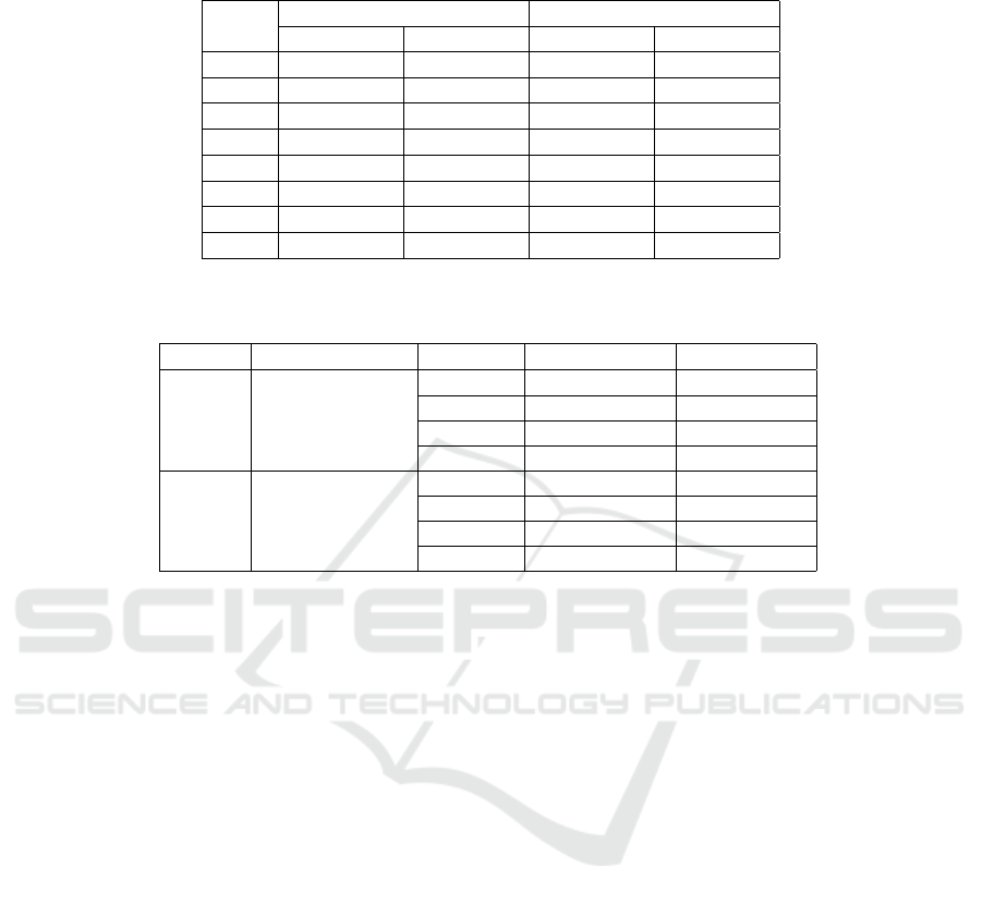
Table 1: Performance evaluation of CGLearn and ERM in linear single environmental setups. The table shows the Mean

Squared Errors (MSE) for causal and noncausal variables across 50 trials for each conﬁguration.

Cases

Causal Error (MSE) Noncausal Error (MSE)

CGLearn ERM CGLearn ERM

FOU 1.28 ± 0.40 1.57 ± 0.13 0.61 ± 0.19 0.54 ± 0.05

FOS 1.40 ± 0.43 1.61 ± 0.10 0.53 ± 0.17 0.52 ± 0.06

FEU 0.13 ± 0.05 0.20 ± 0.04 7.22 ± 2.15 8.28 ± 0.28

FES 0.16 ± 0.06 0.20 ± 0.04 7.47 ± 2.23 8.36 ± 0.30

POU 0.28 ± 0.11 0.37 ± 0.08 0.51 ± 0.18 0.48 ± 0.11

POS 0.34 ± 0.13 0.39 ± 0.07 0.46 ± 0.17 0.48 ± 0.10

PEU 0.24 ± 0.10 0.32 ± 0.07 5.11 ± 1.57 5.83 ± 0.43

PES 0.26 ± 0.10 0.31 ± 0.06 5.21 ± 1.58 5.81 ± 0.36

Table 2: Performance comparison in nonlinear experimental setups for regression tasks. The table shows the RMSE for

training and test environments across 10 trials.

Dataset # Optimal Envs. Method RMSE (Train) RMSE (Test)

Boston 7

ERM 3.57 ± 0.11 6.43 ± 0.45

IRM 3.79 ± 0.33 6.99 ± 0.74

BIRM 3.77 ± 0.50 7.70 ± 0.52

CGLearn 1.91 ± 0.26 5.49 ± 0.28

Yacht 5

ERM 0.21 ± 0.04 3.47 ± 1.15

IRM 2.90 ± 0.03 4.36 ± 0.38

BIRM 0.71 ± 0.19 3.15 ± 0.75

CGLearn 0.48 ± 0.23 2.29 ± 0.42

sistency leads to less dependence on spurious features

and thus better generalization.

Classiﬁcation Tasks. For the classiﬁcation tasks,

we evaluated the performance on two real-world clas-

siﬁcation datasets: the Wine Quality dataset for red

and white wines from the UCI repository (Cortez

et al., 2009). The Wine Quality dataset for red wine

has 1599 instances and 11 attributes, while the dataset

for white wine has 4898 instances and 11 attributes.

The goal is to model wine quality based on physic-

ochemical tests, such as ﬁxed acidity, volatile acid-

ity, citric acid, residual sugar, pH, and etc. Similar

to the regression tasks, we used K-means clustering

to generate diverse environments and determined the

optimal number of environments using the Silhouette

method, ﬁnding 4 as the optimal number of environ-

ments for both classiﬁcation datasets. We then gener-

ated all possible test cases where each environment

was considered the test environment once, and the

rest were used as training environments (as we did

with the regression tasks). We averaged the perfor-

mance over all possible test cases and conducted the

process for 10 random trials. We used accuracy and

F1-score as evaluation metrics, with the results shown

in Table 3. As expected, all methods performed bet-

ter in training environments compared to test environ-

ments. However, we found that CGLearn achieved

higher accuracy and F1-scores, which are desirable,

and the superior performance was statistically signiﬁ-

cant for the F1-score on the Wine Quality Red dataset.

It also had signiﬁcantly better accuracy on the Wine

Quality White dataset. Similar to the regression tasks,

CGLearn demonstrated better predictive power and

generalization over ERM, IRM, and BIRM for the

classiﬁcation tasks.

Limitations of CGLearn with Invariant Spuri-

ous Features. We evaluated CGLearn on the Col-

ored MNIST dataset, a synthetic binary classiﬁcation

task derived from MNIST (LeCun et al., 1995) and

proposed in the IRM study (Arjovsky et al., 2019).

This dataset introduces color as a spurious feature that

strongly correlates with the label in the training envi-

ronments but has the correlation reversed in the test

environment. We applied the nonlinear implemen-

tation of CGLearn and compared it with the results

of ERM and IRM as reported in the IRM study (Ar-

jovsky et al., 2019). Over 10 trials, ERM achieved a

training accuracy of 87.4 ± 0.2 and a test accuracy of

17.1 ± 0.6, while IRM achieved a training accuracy

of 70.8 ± 0.9 and a test accuracy of 66.9 ± 2.5. In

our experimental study, CGLearn achieved a training

accuracy of 93.1 ± 0.8 and a test accuracy of 29.1 ±

0.8. While CGLearn slightly outperformed ERM in

the test environment, it still struggled to generalize.

This limitation arises because CGLearn imposes gra-

dient consistency on the training environments to dis-

CGLearn: Consistent Gradient-Based Learning for Out-of-Distribution Generalization

109

Table 3: Performance comparison in nonlinear setups for classiﬁcation tasks. The table shows accuracy and F1-score for

training and test environments across 10 trials. WQ Red and WQ White represent the Wine Quality Red and Wine Quality

White datasets respectively.

Dataset # Optimal Envs. Method Accuracy (Train) Accuracy (Test) F1-score (Train) F1-score (Test)

WQ Red 4

ERM 62.07 ± 0.34 58.08 ± 1.72 0.692 ± 0.004 0.535 ± 0.010

IRM 63.68 ± 0.19 58.70 ± 1.54 0.644 ± 0.003 0.542 ± 0.014

BIRM 64.94 ± 0.37 57.97 ± 0.93 0.626 ± 0.004 0.536 ± 0.011

CGLearn 61.59 ± 0.44 59.60 ± 0.46 0.638 ± 0.008 0.553 ± 0.007

WQ White 4

ERM 58.73 ± 0.22 51.15 ± 0.34 0.590 ± 0.002 0.447 ± 0.008

IRM 58.82 ± 0.26 51.60 ± 0.40 0.566 ± 0.003 0.450 ± 0.013

BIRM 58.04 ± 0.18 51.87 ± 0.32 0.530 ± 0.006 0.460 ± 0.026

CGLearn 58.23 ± 0.38 52.33 ± 0.32 0.555 ± 0.005 0.460 ± 0.007

tinguish invariant features from spurious ones. How-

ever, in the Colored MNIST setup, the spurious fea-

ture (color) is consistent across both training environ-

ments, leading CGLearn to erroneously treat it as an

invariant feature. Consequently, CGLearn relies on

color and performs poorly in the test environment.

This highlights a limitation of the proposed method,

as it may fail to meet expectations in scenarios where

spurious relationships remain invariant across envi-

ronments. To improve CGLearn’s generalization, fu-

ture work should focus on adapting the method to ac-

count for the varying nature of spurious features, even

when they appear consistent across training environ-

ments.

4 CONCLUSIONS

In this study, we presented CGLearn, a novel ap-

proach for developing robust and predictive machine

learning models by leveraging gradient consistency

across multiple environments. By focusing on the

agreement of gradients, CGLearn effectively identi-

ﬁes and utilizes invariant features, leading to supe-

rior generalization and reduced reliance on spurious

correlations. Our extensive experiments on both syn-

thetic and real-world datasets, including regression

and classiﬁcation tasks, demonstrated that CGLearn

outperforms traditional ERM and state-of-the-art in-

variant learners like ICP, IRM, and BIRM, achieving

lower errors and better generalization in diverse sce-

narios. Notably, even in the absence of predeﬁned

environments, we demonstrated that CGLearn can be

effectively applied to different subsamples of data,

leading to better predictive models than regular ERM.

This ﬂexibility enhances the applicability of CGLearn

in a wide range of real-world scenarios where many

state-of-the-art methods require diverse and deﬁned

environments for OOD generalization.

Despite its strengths, CGLearn has limitations,

particularly in scenarios where spurious features are

invariant across environments, as observed in the Col-

ored MNIST experiments. Such cases violate our as-

sumption as generally we expect and observe causal

features to be stable and invariant in nature whereas

spurious features do not (Woodward, 2005; Wang

et al., 2022). CGLearn erroneously considers these

invariant but spurious features as reliable, impacting

its generalization performance. Addressing this lim-

itation and adapting CGLearn to better handle such

cases is a promising direction for future research.

Overall, CGLearn provides a signiﬁcant step for-

ward in the ﬁeld of robust machine learning by ef-

fectively harnessing causal invariance. Our work

opens new avenues for developing models that are not

only highly predictive but also resilient to distribution

shifts, paving the way for more reliable applications

in real-world settings.

ACKNOWLEDGEMENTS

Research was sponsored by the Army Research Of-

ﬁce under Grant Number W911NF-22-1-0035 and by

the National Science Foundation under Award Num-

ber 2218841. The views and conclusions contained in

this document are those of the authors and should not

be interpreted as representing the ofﬁcial policies, ei-

ther expressed or implied, of the Army Research Of-

ﬁce or the U.S. Government. The U.S. Government

is authorized to reproduce and distribute reprints for

Government purposes notwithstanding any copyright

notation herein.

REFERENCES

Andrews, B., Spirtes, P., and Cooper, G. F. (2020). On the

completeness of causal discovery in the presence of la-

tent confounding with tiered background knowledge.

In International Conference on Artiﬁcial Intelligence

and Statistics, pages 4002–4011. PMLR.

Arjovsky, M., Bottou, L., Gulrajani, I., and Lopez-Paz, D.

ICPRAM 2025 - 14th International Conference on Pattern Recognition Applications and Methods

110

(2019). Invariant risk minimization. arXiv preprint

arXiv:1907.02893.

Bose, R. and Roy, A. M. (2024). Invariance embedded

physics-infused deep neural network-based sub-grid

scale models for turbulent ﬂows. Engineering Appli-

cations of Artiﬁcial Intelligence, 128:107483.

Chickering, D. M. (2002). Optimal structure identiﬁcation

with greedy search. Journal of Machine Learning Re-

search, 3(Nov):507–554.

Chowdhury, J., Fricke, C., Bamidele, O., Bello, M., Yang,

W., Heyden, A., and Terejanu, G. (2024). Invariant

molecular representations for heterogeneous cataly-

sis. Journal of Chemical Information and Modeling,

64(2):327–339.

Chowdhury., J., Rashid., R., and Terejanu., G. (2023). Eval-

uation of induced expert knowledge in causal struc-

ture learning by notears. In Proceedings of the 12th

International Conference on Pattern Recognition Ap-

plications and Methods - ICPRAM, pages 136–146.

INSTICC, SciTePress.

Chowdhury, J. and Terejanu, G. (2023). Cd-notears: Con-

cept driven causal structure learning using notears. In

2023 International Conference on Machine Learning

and Applications (ICMLA), pages 808–813. IEEE.

Colombo, D., Maathuis, M. H., Kalisch, M., and Richard-

son, T. S. (2012). Learning high-dimensional directed

acyclic graphs with latent and selection variables. The

Annals of Statistics, pages 294–321.

Cortez, P., Cerdeira, A., Almeida, F., Matos, T., and Reis, J.

(2009). Wine Quality. UCI Machine Learning Repos-

itory. DOI: https://doi.org/10.24432/C56S3T.

Ge, Y., Arik, S.

O., Yoon, J., Xu, A., Itti, L., and Pﬁster,

T. (2022). Invariant structure learning for better gen-

eralization and causal explainability. arXiv preprint

arXiv:2206.06469.

Gencoglu, O. and Gruber, M. (2020). Causal modeling

of twitter activity during covid-19. Computation,

8(4):85.

Gerritsma, J., Onnink, R., and Versluis, A. (2013). Yacht

Hydrodynamics. UCI Machine Learning Repository.

DOI: https://doi.org/10.24432/C5XG7R.

Harrison, D. and Rubinfeld, D. L. (1978). Hedonic prices

and the demand for clean air. J. Environ. Econ. and

Management. UCI Machine Learning Repository,

http://lib.stat.cmu.edu/datasets/boston.

He, Y., Shen, Z., and Cui, P. (2021). Towards non-iid im-

age classiﬁcation: A dataset and baselines. Pattern

Recognition, 110:107383.

Huang, B., Zhang, K., Lin, Y., Sch

olkopf, B., and Glymour,

C. (2018). Generalized score functions for causal dis-

covery. In Proceedings of the 24th ACM SIGKDD

international conference on knowledge discovery &

data mining, pages 1551–1560.

Jiang, G.-q., Liu, J., Ding, Z., Guo, L., and Lin, W. (2023).

Accelerating large batch training via gradient signal to

noise ratio (gsnr). arXiv preprint arXiv:2309.13681.

Kaiser, M. and Sipos, M. (2022). Unsuitability of notears

for causal graph discovery when dealing with di-

mensional quantities. Neural Processing Letters,

54(3):1587–1595.

Koyama, M. and Yamaguchi, S. (2020). Out-of-distribution

generalization with maximal invariant predictor.

Lachapelle, S., Brouillard, P., Deleu, T., and Lacoste-Julien,

S. (2019). Gradient-based neural dag learning. arXiv

preprint arXiv:1906.02226.

LeCun, Y., Jackel, L. D., Bottou, L., Cortes, C., Denker,

J. S., Drucker, H., Guyon, I., Muller, U. A., Sackinger,

E., Simard, P., et al. (1995). Learning algorithms

for classiﬁcation: A comparison on handwritten digit

recognition. Neural networks: the statistical mechan-

ics perspective, 261(276):2.

Lin, Y., Dong, H., Wang, H., and Zhang, T. (2022).

Bayesian invariant risk minimization. In Proceedings

of the IEEE/CVF Conference on Computer Vision and

Pattern Recognition, pages 16021–16030.

Liu, J., Chen, Y., and Zhao, J. (2021). Knowledge enhanced

event causality identiﬁcation with mention masking

generalizations. In Proceedings of the twenty-ninth

international conference on international joint confer-

ences on artiﬁcial intelligence, pages 3608–3614.

Liu, J., Jiang, G., Bai, Y., Chen, T., and Wang, H.

(2020). Understanding why neural networks gener-

alize well through gsnr of parameters. arXiv preprint

arXiv:2001.07384.

Lloyd, S. (1982). Least squares quantization in pcm. IEEE

transactions on information theory, 28(2):129–137.

Ming, Y., Yin, H., and Li, Y. (2022). On the impact of

spurious correlation for out-of-distribution detection.

In Proceedings of the AAAI conference on artiﬁcial

intelligence, volume 36, pages 10051–10059.

Montavon, G., Hansen, K., Fazli, S., Rupp, M., Biegler,

F., Ziehe, A., Tkatchenko, A., Lilienfeld, A., and

uller, K.-R. (2012). Learning invariant representa-

tions of molecules for atomization energy prediction.

Advances in neural information processing systems,

25.

Ng, I., Ghassami, A., and Zhang, K. (2020). On the role of

sparsity and dag constraints for learning linear dags.

Advances in Neural Information Processing Systems,

33:17943–17954.

Ng, I., Zhu, S., Fang, Z., Li, H., Chen, Z., and Wang, J.

(2022). Masked gradient-based causal structure learn-

ing. In Proceedings of the 2022 SIAM International

Conference on Data Mining (SDM), pages 424–432.

SIAM.

Ormaniec, W., Sussex, S., Lorch, L., Sch

olkopf, B., and

Krause, A. (2024). Standardizing structural causal

models. arXiv preprint arXiv:2406.11601.

O’Donnell, R. T., Nicholson, A. E., Han, B., Korb, K. B.,

Alam, M. J., and Hope, L. R. (2006). Causal discov-

ery with prior information. In AI 2006: Advances in

Artiﬁcial Intelligence: 19th Australian Joint Confer-

ence on Artiﬁcial Intelligence, Hobart, Australia, De-

cember 4-8, 2006. Proceedings 19, pages 1162–1167.

Springer.

Parascandolo, G., Neitz, A., Orvieto, A., Gresele, L., and

Sch

olkopf, B. (2020). Learning explanations that are

hard to vary. arXiv preprint arXiv:2009.00329.

Pearl, J. (2009). Causality. Cambridge university press.

CGLearn: Consistent Gradient-Based Learning for Out-of-Distribution Generalization

111

Peters, J., B

uhlmann, P., and Meinshausen, N. (2016).

Causal inference by using invariant prediction: identi-

ﬁcation and conﬁdence intervals. Journal of the Royal

Statistical Society Series B: Statistical Methodology,

78(5):947–1012.

Rame, A., Dancette, C., and Cord, M. (2022). Fishr: In-

variant gradient variances for out-of-distribution gen-

eralization. In International Conference on Machine

Learning, pages 18347–18377. PMLR.

Ramsey, J., Glymour, M., Sanchez-Romero, R., and Gly-

mour, C. (2017). A million variables and more: the

fast greedy equivalence search algorithm for learn-

ing high-dimensional graphical causal models, with

an application to functional magnetic resonance im-

ages. International Journal of Data Science and Ana-

lytics, 3:121–129.

Reisach, A., Seiler, C., and Weichwald, S. (2021). Beware

of the simulated dag! causal discovery benchmarks

may be easy to game. Advances in Neural Information

Processing Systems, 34:27772–27784.

Reisach, A., Tami, M., Seiler, C., Chambaz, A., and Weich-

wald, S. (2024). A scale-invariant sorting criterion to

ﬁnd a causal order in additive noise models. Advances

in Neural Information Processing Systems, 36.

Rosenfeld, E., Ravikumar, P. K., and Risteski, A. (2021).

The risks of invariant risk minimization. In Interna-

tional Conference on Learning Representations.

Rousseeuw, P. J. (1987). Silhouettes: a graphical aid to

the interpretation and validation of cluster analysis.

Journal of computational and applied mathematics,

20:53–65.

Sagawa, S., Raghunathan, A., Koh, P. W., and Liang, P.

(2020). An investigation of why overparameterization

exacerbates spurious correlations. In International

Conference on Machine Learning, pages 8346–8356.

PMLR.

Santillan, B. G. (2023). A step towards the applicability of

algorithms based on invariant causal learning on ob-

servational data. arXiv preprint arXiv:2304.02286.

Shi, Y., Seely, J., Torr, P. H., Siddharth, N., Hannun, A.,

Usunier, N., and Synnaeve, G. (2021). Gradient

matching for domain generalization. arXiv preprint

arXiv:2104.09937.

Shin, D. (2021). The effects of explainability and causabil-

ity on perception, trust, and acceptance: Implications

for explainable ai. International journal of human-

computer studies, 146:102551.

Spirtes, P., Glymour, C., and Scheines, R. (2001). Causa-

tion, prediction, and search. MIT press.

Torralba, A. and Efros, A. A. (2011). Unbiased look at

dataset bias. In CVPR 2011, pages 1521–1528. IEEE.

Wang, J., Lan, C., Liu, C., Ouyang, Y., Qin, T., Lu, W.,

Chen, Y., Zeng, W., and Philip, S. Y. (2022). General-

izing to unseen domains: A survey on domain gener-

alization. IEEE transactions on knowledge and data

engineering, 35(8):8052–8072.

Wang, Q., Zheng, Y., Yang, G., Jin, W., Chen, X., and

Yin, Y. (2017). Multiscale rotation-invariant convolu-

tional neural networks for lung texture classiﬁcation.

IEEE journal of biomedical and health informatics,

22(1):184–195.

Wang, T., Sridhar, R., Yang, D., and Wang, X. (2021).

Identifying and mitigating spurious correlations for

improving robustness in nlp models. arXiv preprint

arXiv:2110.07736.

Wei, D., Gao, T., and Yu, Y. (2020). Dags with no fears:

A closer look at continuous optimization for learning

bayesian networks. Advances in Neural Information

Processing Systems, 33:3895–3906.

Woodward, J. (2005). Making things happen: A theory of

causal explanation. Oxford university press.

Yu, Y., Chen, J., Gao, T., and Yu, M. (2019). Dag-gnn:

Dag structure learning with graph neural networks. In

International conference on machine learning, pages

7154–7163. PMLR.

Zadrozny, B. (2004). Learning and evaluating classi-

ﬁers under sample selection bias. In Proceedings of

the twenty-ﬁrst international conference on Machine

learning, page 114.

Zheng, X., Aragam, B., Ravikumar, P. K., and Xing, E. P.

(2018). Dags with no tears: Continuous optimization

for structure learning. Advances in neural information

processing systems, 31.

Zheng, X., Dan, C., Aragam, B., Ravikumar, P., and Xing,

E. (2020). Learning sparse nonparametric dags. In In-

ternational Conference on Artiﬁcial Intelligence and

Statistics, pages 3414–3425. Pmlr.

ICPRAM 2025 - 14th International Conference on Pattern Recognition Applications and Methods

112