Neighbor Embedding Projection and Graph Convolutional Networks for
Image Classification
Gustavo Rosseto Leticio
a
, Vinicius Atsushi Sato Kawai
b
, Lucas Pascotti Valem
c
and Daniel Carlos Guimar
˜
aes Pedronette
d
Department of Statistics, Applied Mathematics, and Computing (DEMAC),
S
˜
ao Paulo State University (UNESP), Rio Claro, Brazil
Keywords:
Semi-Supervised Learning, Graph Convolutional Networks, Neighbor Embedding Projection.
Abstract:
The exponential increase in image data has heightened the need for machine learning applications, particularly
in image classification across various fields. However, while data volume has surged, the availability of labeled
data remains limited due to the costly and time-intensive nature of labeling. Semi-supervised learning offers
a promising solution by utilizing both labeled and unlabeled data; it employs a small amount of labeled data
to guide learning on a larger unlabeled set, thus reducing the dependency on extensive labeling efforts. Graph
Convolutional Networks (GCNs) introduce an effective method by applying convolutions in graph space,
allowing information propagation across connected nodes. This technique captures individual node features
and inter-node relationships, facilitating the discovery of intricate patterns in graph-structured data. Despite
their potential, GCNs remain underutilized in image data scenarios, where input graphs are often computed
using features extracted from pre-trained models without further enhancement. This work proposes a novel
GCN-based approach for image classification, incorporating neighbor embedding projection techniques to
refine the similarity graph and improve the latent feature space. Similarity learning approaches, commonly
employed in image retrieval, are also integrated into our workflow. Experimental evaluations across three
datasets, four feature extractors, and three GCN models revealed superior results in most scenarios.
1 INTRODUCTION
The rapid expansion of multimedia data presents
increasing challenges in image classification tasks,
where effective utilization of both labeled and un-
labeled data is essential (Datta et al., 2008). This
surge has driven the adoption of semi-supervised
learning techniques, particularly in cases where man-
ual labeling is impractical or costly (Li et al.,
2019). In this context, Graph Convolutional Networks
(GCNs) (Kipf and Welling, 2017) have emerged as
a powerful tool in semi-supervised frameworks. Un-
like traditional classifiers, which rely solely on feature
representations, GCNs also require a graph that en-
codes relationships between data samples. This dual
input allows GCNs to leverage graph-based represen-
tations to capture structural dependencies in the data,
a
https://orcid.org/0009-0008-3715-8991
b
https://orcid.org/0000-0003-0153-7910
c
https://orcid.org/0000-0002-3833-9072
d
https://orcid.org/0000-0002-2867-4838
improving classification performance even with lim-
ited labeled samples.
However, the effectiveness of GCNs is closely tied
to the quality of the underlying graph. An accurately
constructed graph can reinforce the model’s ability to
capture meaningful inter-sample relationships (Valem
et al., 2023a; Miao et al., 2021), whereas a poorly
constructed graph may undermine classification per-
formance. This dependency underscores the need for
methods that refine data representation, ensuring that
the graph structure aligns more closely with the in-
trinsic patterns in the data.
In this context, manifold learning methods, par-
ticularly those based on neighbor embedding projec-
tions such as Uniform Manifold Approximation and
Projection (UMAP) (McInnes et al., 2018), offer a
promising approach to enhancing GCN performance.
UMAP, known for its capability to preserve both local
and global structures in a lower-dimensional space,
enables a more discriminative organization of high-
dimensional feature data. This refined representation
provides a better foundation for similarity graph con-
Leticio, G. R., Kawai, V. A. S., Valem, L. P. and Pedronette, D. C. G.
Neighbor Embedding Projection and Graph Convolutional Networks for Image Classification.
DOI: 10.5220/0013260500003912
Paper published under CC license (CC BY-NC-ND 4.0)
In Proceedings of the 20th International Joint Conference on Computer Vision, Imaging and Computer Graphics Theory and Applications (VISIGRAPP 2025) - Volume 2: VISAPP, pages
511-518
ISBN: 978-989-758-728-3; ISSN: 2184-4321
Proceedings Copyright © 2025 by SCITEPRESS – Science and Technology Publications, Lda.
511

struction and, consequently, GCN training. Addition-
ally, recent advancements in manifold learning have
highlighted their potential not only for neighbor em-
bedding projection but also for improving retrieval
quality in various image retrieval applications (Leti-
cio et al., 2024; Kawai et al., 2024).
Rank-based manifold learning methods (Pe-
dronette et al., 2019; Bai et al., 2019) refine data
representations by enhancing the global structure of
similarity relationships within ranked lists. These
methods improve neighborhood quality by exploring
the contextual similarity information encoded in the
top-ranked neighbors. The refined ranked lists can
then be used to construct more representative graphs
for GCNs (Valem et al., 2023a). Consequently, a
GCN trained on this enhanced graph is more likely to
benefit from these enriched relationships, potentially
yielding more accurate classification results.
Building on these insights, this paper proposes
a novel workflow to improve image classification
through GCNs by integrating UMAP and re-ranking
methods. High-dimensional features are extracted
from deep learning models and projected into a lower-
dimensional space with UMAP to capture intrinsic
data relationships. Ranked lists generated in this
space are refined using rank-based manifold learning
methods. This refined similarity information guides
the graph construction, which serves as the input for
GCN training. By integrating neighbor embedding
projection, re-ranking, and graph construction within
a semi-supervised GCN framework, the proposed ap-
proach aims to achieve more accurate classifications
through improved data representations.
To the best of our knowledge, this is the first
approach to exploit neighbor embedding projection
techniques for improving the similarity graphs used
by GCNs. Our proposed framework was evaluated
across three datasets, four feature extraction models,
and three GCN architectures. The results demonstrate
significant improvements, with classification accu-
racy gains reaching +19.62% in the best case, under-
scoring the effectiveness and potential of our work.
2 PROPOSED APPROACH
The proposed approach combines neighbor embed-
ding projection and GCNs to improve image classi-
fication, as shown in Figure 1. It starts with feature
extraction using deep learning models (e.g., CNNs,
Transformers) to capture high-dimensional charac-
teristics ([A-C]). These features are reduced with
UMAP, preserving neighborhood relationships ([D]).
Manifold learning refines similarity rankings ([E-G]),
which are then used to construct a graph encoding
contextual dependencies ([H]). Finally, a GCN learns
enriched representations for better classification per-
formance ([I-J]).
In this way, this section presents the proposed ap-
proach, and is divided as follows: Section 2.1 presents
the Neighbor Embedding Projection technique used
in our approach. In Section 2.2, we discuss about
Rank-Based manifold learning. Finally, Section 2.3
explains the graph construction step and the Graph
Convolutional Networks (GCNs).
2.1 Neighborhood Embedding
Projection Based on UMAP
Neighbor embedding methods assign probabilities to
model attractive and repulsive forces between nearby
and distant points, in other words, how similar or dif-
ferent points are (Ghojogh et al., 2021). Two widely
used methods for visualizing high-dimensional data
based on this concept are t-distributed Stochastic
Neighbor Embedding (t-SNE) (van der Maaten and
Hinton, 2008) and Uniform Manifold Approximation
and Projection (UMAP) (McInnes et al., 2018).
In our approach, UMAP plays a key role in creat-
ing a lower-dimensional embedding of the extracted
features while preserving both local and global neigh-
borhood relationships, crucial for ranking and graph
construction tasks. UMAP begins by building a
high-dimensional k-nearest neighbor (k-NN) graph
to capture relationships in high-dimensional data. It
then optimizes a projection that aligns these relation-
ships into a compact, low-dimensional representation,
without restrictions on the embedding dimension, al-
lowing flexibility for different applications (Ghojogh
et al., 2021). This process provides a condensed view
of the data’s intrinsic structure, making UMAP partic-
ularly valuable for generating rankings based on sim-
ilarity for image retrieval tasks (Leticio et al., 2024).
2.2 Similarity and Rank-Based
Manifold Learning
The similarity ranking task plays a fundamental role
in organizing image data for tasks such as graph con-
struction and image retrieval. In this process, each
image in a dataset is represented as a feature vector,
and its similarity to other images is measured using a
distance function, such as Euclidean distance. Based
on these measurements, ranked lists are created by or-
dering images according to their closeness to a query
image. These lists provide a structured way to iden-
tify the most similar images within the dataset (Kib-
riya and Frank, 2007; Valem et al., 2023a). However,
VISAPP 2025 - 20th International Conference on Computer Vision Theory and Applications
512

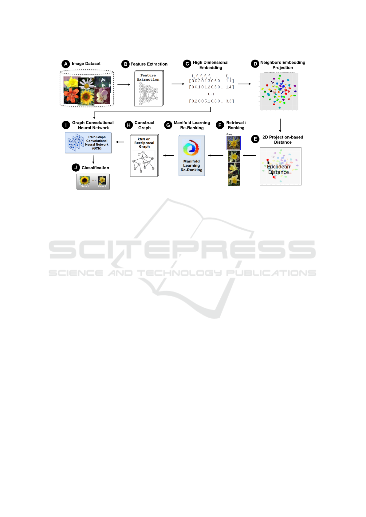
Figure 1: Proposed Method: Graph Convolution Networks and Neighbor Embedding Projection for improved classification.
comparing elements in pairs can overlook contextual
information and the more complex similarity relation-
ships that can be found in the data structure.
Manifold learning is a term frequently seen in the
literature, with a variety of definitions. Generally,
manifold learning methods aim to identify and uti-
lize the intrinsic manifold structure to provide a more
meaningful measure of similarity or distance (Jiang
et al., 2011). In this way, rank-based manifold learn-
ing methods are capable of refining the similarity
rankings by leveraging information encoded in the
ranked lists of nearest neighbors.
In this work, four rank-based methods were em-
ployed: Cartesian Product of Ranking References
(CPRR) (Valem et al., 2018), Log-based Hypergraph
of Ranking References (LHRR) (Pedronette et al.,
2019), Rank-based Diffusion Process with Assured
Convergence (RDPAC) (Pedronette et al., 2021), and
Rank Flow Embedding (RFE) (Valem et al., 2023b).
These methods iteratively refine ranked lists by incor-
porating relevant contextual information, resulting in
more discriminative similarity graphs, which are sub-
sequently used in GCN training.
2.3 Graph Construction and Graph
Convolutional Networks
The process of graph construction is fundamental for
leveraging Graph Convolutional Networks (GCNs) in
semi-supervised learning tasks. In this work, ranked
lists are used to build similarity graphs, adopting two
approaches: the traditional kNN graph and the recip-
rocal kNN graph. The kNN graph connects each node
to its k most similar neighbors, providing a straight-
forward representation of local similarity. In contrast,
the reciprocal kNN graph adds a layer of refinement
by requiring mutual inclusion in each other’s k nearest
neighbors, reducing noise by eliminating one-sided
links (Valem et al., 2023a).
The quality of the constructed graph directly im-
pacts GCN performance. A well-constructed graph
preserves meaningful relationships between nodes,
enabling effective information aggregation and prop-
agation, while noisy connections can hinder learning
by introducing irrelevant or misleading relationships.
Once the graph is constructed, GCNs operate on
this structured data by learning representations for
each node. A GCN works by aggregating informa-
tion from a node’s neighbors and combining it with
the node’s own features to generate a new, enriched
representation (Kipf and Welling, 2017). This pro-
cess can be understood as a way of “sharing” infor-
mation across the graph, where each node iteratively
learns from its local neighborhood. Through multi-
ple layers, a GCN can propagate information across
the graph, enabling nodes to capture both local and
global structural dependencies.
In our work, we evaluate the original GCN and
two variants: Simple Graph Convolution (SGC) (Wu
et al., 2019), a simplified version of the original
GCN, designed to lower computational complexity
by removing non-linear transformations between lay-
ers; Approximate Personalized Propagation of Neu-
ral Predictions (APPNP) (Klicpera et al., 2019), this
model combines the GCN with the PageRank algo-
rithm, utilizing a propagation strategy based on a
modified PageRank approach.
Neighbor Embedding Projection and Graph Convolutional Networks for Image Classification
513

3 EXPERIMENTAL EVALUATION
This section presents the experimental evaluation of
the proposed approach. Section 3.1 details the ex-
perimental protocol. Semi-supervised classification
and visualization results are provided in Section 3.2,
while comparisons with state-of-the-art are discussed
in Section 3.3. Furthermore, a link is added for sup-
plementary material containing additional informa-
tion
1
.
3.1 Experimental Protocol
Three public datasets were selected for the experi-
mental analysis: Flowers17 (Nilsback and Zisserman,
2006) includes 1,360 images of 17 flower species with
80 images per class; Corel5k (Liu and Yang, 2013)
contains 5,000 images across 100 categories with 50
images each, covering themes such as vehicles and
animals; and the CUB-200 dataset (Wah et al., 2011),
a benchmark for image classification, includes 11,788
images covering 200 bird species.
The experiments were conducted using features
extracted from four different models: DinoV2 (ViT-
B14 as the backbone) (Oquab et al., 2023), Swin
Transformer (Liu et al., 2021), VIT-B16 (Dosovitskiy
et al., 2021), and ResNet152 (He et al., 2016).
For all features, the BallTree algorithm (Kibriya
and Frank, 2007) was employed to compute ranked
lists based on Euclidean distances, ensuring effi-
cient neighbor retrieval. The dimensionality reduc-
tion step used UMAP with the following parame-
ters: n components = 2, cosine as the metric, and
random state = 42.
For the manifold learning methods, we employed
the default parameters from the pyUDLF frame-
work (Leticio et al., 2023), modifying only the param-
eter K, which was set to K = 40 across all datasets.
This is distinct from the graph parameter k, where we
also set k to 40 in every case.
During the semi-supervised classification step us-
ing GCN, a 10-fold cross-validation was conducted.
In each execution, one fold was used for training,
while the remaining 90% of the data served as un-
labeled test data. This process was repeated 10 times,
ensuring that each fold was used as the training set at
least once. Since we performed five rounds of 10-fold
cross-validation, the reported results represent the av-
erage of 50 runs (5 executions of 10 folds).
We used the Adam optimizer with a learning rate
of 10
−4
for all models and trained for 200 epochs.
The default configuration was 256 neurons, except for
GCN-SGC, which doesn’t require this parameter, and
1
Supplementary files: visapp2025.lucasvalem.com
for the CUB-200 dataset, where we used 64 neurons.
Additional detailed information about the GCNs set-
tings, is provided in the supplementary material.
3.2 Results and Visualization
The classification performance across the Flowers17,
Corel5k, and CUB-200 datasets highlights the impact
of using UMAP for feature projection and re-ranking
techniques (CPRR, LHRR, RDPAC, RFE) to improve
baseline GCN models relying on kNN or reciprocal
kNN graphs.
For the Flowers17 dataset, as shown in Table 1,
baseline GCN models using reciprocal kNN graphs
perform well, with the GCN-SGC model achieving
96.92% accuracy using ViT-b16 features. Adding
UMAP and LHRR further enhances accuracy to
98.28%, demonstrating the benefits of neighbor em-
bedding projection in refining feature representa-
tion. With DinoV2 features, the GCN-SGC baseline
achieves 99.81%, and combining UMAP with CPRR
or LHRR reaches 100%.
The Corel5k dataset (Table 2) shows similar im-
provements. For instance, the GCN-APPNP model
with kNN graphs and ViT-b16 features achieves
87.0%, while UMAP with LHRR raises accuracy to
95.01%. These consistent gains confirm the effective-
ness of UMAP combined with manifold re-ranking.
On the CUB-200 dataset (Table 3), the advan-
tage of UMAP and re-ranking is even clearer. The
GCN-APPNP model, using UMAP, kNN graphs,
and CPRR, achieves 75.13% accuracy, significantly
improving over the baseline of 55.51% (+19.62%).
However, cases such as ResNet features on the same
dataset show that models without UMAP can some-
times perform better, suggesting UMAP’s effective-
ness varies with the feature quality and dataset. Future
work could further explore when UMAP most effec-
tively enhances feature separation.
The visualization results (Figure 2) illustrate these
findings. For Flowers17, UMAP-reduced ResNet152
features (plot a) show mixed class clusters, mak-
ing separation difficult. GCN embeddings trained
on a kNN graph built from original features (plot b)
slightly improve class distinction, while those trained
on UMAP-reduced features (plot c) yield more dis-
tinct clusters. This comparison highlights how each
transformation step enhances class clustering and sep-
aration in the feature space.
Table 4 presents the average results across
datasets, showing that the proposed approach consis-
tently outperforms baseline models. The mean ac-
curacy for kNN graphs improved from 83.13% to
86.91% with UMAP and CPRR, while reciprocal
VISAPP 2025 - 20th International Conference on Computer Vision Theory and Applications
514

Table 1: Impact of neighbor embedding projection and manifold learning methods on the classification accuracy of three GCN
models for the Flowers17 dataset. The best results are highlighted in bold.
Classifier Specification Feature
GCN Graph Projection Re-Rank
Resnet152 DinoV2 SwinTF VIT-B16
GCN-Net
kNN — — 79.43 ± 0.0985 99.82 ± 0.0303 97.17 ± 0.0231 92.70 ± 0.1045
kNN UMAP — 83.67 ± 0.2122 100.0 ± 0.0 99.81 ± 0.0000 97.46 ± 0.1389
kNN UMAP CPRR 83.25 ± 0.3316 100.0 ± 0.0 99.85 ± 0.0080 97.92 ± 0.0671
kNN UMAP LHRR 82.90 ± 0.2838 100.0 ± 0.0 99.85 ± 0.0000 97.97 ± 0.1211
kNN UMAP RDPAC 82.84 ± 0.2438 100.0 ± 0.0 99.61 ± 0.0095 97.70 ± 0.1822
kNN UMAP RFE 81.88 ± 0.3561 99.98 ± 0.0359 99.75 ± 0.0320 97.81 ± 0.0943
Rec — — 83.76 ± 0.0640 99.78 ± 0.0246 99.81 ± 0.0246 96.96 ± 0.0663
Rec UMAP — 83.62 ± 0.2752 99.84 ± 0.0881 99.75 ± 0.0167 97.74 ± 0.0717
Rec UMAP CPRR 83.00 ± 0.2002 100.0 ± 0.0 99.81 ± 0.0336 97.83 ± 0.0925
Rec UMAP LHRR 83.05 ± 0.1488 100.0 ± 0.0 99.84 ± 0.0103 97.90 ± 0.0333
Rec UMAP RDPAC 82.58 ± 0.1494 100.0 ± 0.0 99.50 ± 0.0061 97.87 ± 0.0423
Rec UMAP RFE 82.42 ± 0.2974 99.89 ± 0.0673 99.82 ± 0.0098 97.55 ± 0.0818
GCN-SGC
kNN — — 79.69 ± 0.0434 99.81 ± 0.0095 97.04 ± 0.0281 92.80 ± 0.0352
kNN UMAP — 84.18 ± 0.0894 100.0 ± 0.0 99.85 ± 0.0000 98.01 ± 0.0349
kNN UMAP CPRR 83.99 ± 0.0686 100.0 ± 0.0 99.85 ± 0.0000 98.36 ± 0.0065
kNN UMAP LHRR 83.59 ± 0.0867 100.0 ± 0.0 99.85 ± 0.0000 98.32 ± 0.0040
kNN UMAP RDPAC 83.47 ± 0.0332 100.0 ± 0.0 99.81 ± 0.0040 98.20 ± 0.0160
kNN UMAP RFE 83.21 ± 0.0844 100.0 ± 0.0 99.85 ± 0.0000 98.25 ± 0.0595
Rec — — 83.99 ± 0.0304 99.91 ± 0.0434 99.78 ± 0.0158 96.92 ± 0.0558
Rec UMAP — 84.32 ± 0.1001 99.87 ± 0.0916 99.85 ± 0.0000 97.98 ± 0.0083
Rec UMAP CPRR 83.79 ± 0.0998 100.0 ± 0.0 99.85 ± 0.0000 98.27 ± 0.0219
Rec UMAP LHRR 83.55 ± 0.1829 100.0 ± 0.0 99.85 ± 0.0000 98.28 ± 0.0489
Rec UMAP RDPAC 83.10 ± 0.0158 100.0 ± 0.0 99.51 ± 0.0040 98.19 ± 0.0225
Rec UMAP RFE 83.00 ± 0.0700 99.95 ± 0.0440 99.81 ± 0.0052 97.95 ± 0.1603
GCN-APPNP
kNN — — 77.03 ± 0.3860 99.82 ± 0.0120 97.46 ± 0.0450 90.15 ± 0.3653
kNN UMAP — 85.05 ± 0.1878 100.0 ± 0.0 99.85 ± 0.0000 98.03 ± 0.0586
kNN UMAP CPRR 84.80 ± 0.1251 100.0 ± 0.0 99.85 ± 0.0000 98.36 ± 0.0155
kNN UMAP LHRR 84.60 ± 0.1800 100.0 ± 0.0 99.85 ± 0.0000 98.33 ± 0.0116
kNN UMAP RDPAC 84.38 ± 0.2368 100.0 ± 0.0 99.85 ± 0.0000 98.25 ± 0.1238
kNN UMAP RFE 84.17 ± 0.1112 100.0 ± 0.0 99.85 ± 0.0000 98.26 ± 0.0183
Rec — — 84.03 ± 0.2363 99.91 ± 0.0464 99.72 ± 0.0061 97.22 ± 0.0434
Rec UMAP — 84.67 ± 0.1000 99.98 ± 0.0327 99.85 ± 0.0000 98.15 ± 0.0425
Rec UMAP CPRR 84.59 ± 0.2291 100.0 ± 0.0 99.85 ± 0.0000 98.40 ± 0.0387
Rec UMAP LHRR 84.39 ± 0.2974 100.0 ± 0.0 99.85 ± 0.0000 98.34 ± 0.0504
Rec UMAP RDPAC 83.81 ± 0.1621 100.0 ± 0.0 99.69 ± 0.0525 98.32 ± 0.0356
Rec UMAP RFE 83.99 ± 0.2978 99.96 ± 0.0368 99.83 ± 0.0083 98.09 ± 0.1254
kNN achieved comparable results with most of its
combinations.
In summary, UMAP and manifold re-ranking con-
sistently enhance graph construction and classifica-
tion performance in semi-supervised GCN frame-
works.
3.3 Comparison with State-of-the-Art
This section compares our approach with the state-of-
the-art “Manifold GCN” (Valem et al., 2023a), tested
on the same datasets, using identical settings: ViT-
B16 features, RDPAC re-ranking model, and graph
structures based on kNN and reciprocal kNN.
Our method achieved higher average accuracy
on Flowers17 and CUB-200, as shown in Table 5,
while remaining competitive with Manifold-GCN on
Corel5k. These results underscore its ability to cap-
ture complex relationships across different GCNs,
graph types, datasets, and features.
4 CONCLUSIONS
In this work, we presented a novel approach for im-
proving image classification accuracy by using neigh-
bor embedding projection approaches in combina-
tion with re-ranking techniques to enhance the input
graph. The experimental results showed that the pro-
posed method revealed better results in most cases
when the neighbor embedding projection was em-
ployed. In some cases, the use of re-ranking was ca-
pable of further improving the accuracy. For future
work, we plan to investigate the use of neighbor em-
bedding projection directly on the input features. We
also intend to employ the approach for other types of
multimedia data (e.g., video and sound).
Neighbor Embedding Projection and Graph Convolutional Networks for Image Classification
515

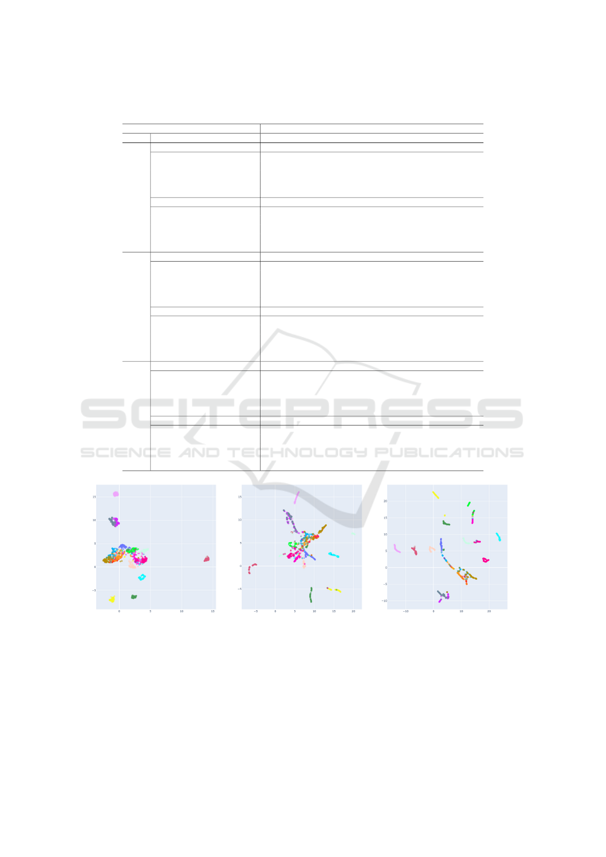
Table 2: Impact of neighbor embedding projection and manifold learning methods on the classification accuracy of three GCN
models for the Corel5K dataset. The best results are highlighted in bold.
Classifier Specification Feature
GCN Graph Projection Re-Rank
Resnet152 DinoV2 SwinTF VIT-B16
GCN-Net
kNN — — 89.31 ± 0.0891 93.11 ± 0.1471 95.84 ± 0.0599 92.52 ± 0.1209
kNN UMAP — 90.64 ± 0.0999 94.41 ± 0.1863 97.26 ± 0.0454 94.18 ± 0.1187
kNN UMAP CPRR 90.83 ± 0.1871 94.09 ± 0.1348 96.91 ± 0.1068 94.50 ± 0.0615
kNN UMAP LHRR 90.66 ± 0.0555 94.47 ± 0.1530 97.14 ± 0.0723 94.48 ± 0.1683
kNN UMAP RDPAC 90.64 ± 0.1941 94.17 ± 0.0750 97.31 ± 0.0861 94.39 ± 0.0704
kNN UMAP RFE 90.46 ± 0.1440 94.09 ± 0.2022 97.20 ± 0.1502 94.53 ± 0.1214
Rec — — 91.63 ± 0.0887 94.88 ± 0.1254 97.59 ± 0.0967 94.56 ± 0.0858
Rec UMAP — 91.28 ± 0.1434 94.40 ± 0.0865 97.74 ± 0.0660 94.80 ± 0.0416
Rec UMAP CPRR 90.97 ± 0.1420 94.78 ± 0.1816 97.47 ± 0.1101 94.56 ± 0.1357
Rec UMAP LHRR 91.06 ± 0.1143 94.75 ± 0.0966 97.55 ± 0.1045 94.70 ± 0.0583
Rec UMAP RDPAC 90.99 ± 0.1200 94.50 ± 0.1153 97.48 ± 0.1274 94.32 ± 0.0893
Rec UMAP RFE 91.00 ± 0.1227 94.54 ± 0.2185 97.66 ± 0.0588 94.61 ± 0.0701
GCN-SGC
kNN — — 89.59 ± 0.0260 93.26 ± 0.0389 95.90 ± 0.0254 93.36 ± 0.0443
kNN UMAP — 91.15 ± 0.0301 94.73 ± 0.0617 97.36 ± 0.0069 94.74 ± 0.0663
kNN UMAP CPRR 91.10 ± 0.0293 94.63 ± 0.0455 97.02 ± 0.0417 94.89 ± 0.0570
kNN UMAP LHRR 91.15 ± 0.0336 94.78 ± 0.1049 97.21 ± 0.0267 94.99 ± 0.0308
kNN UMAP RDPAC 91.06 ± 0.0657 94.45 ± 0.0892 97.41 ± 0.0412 94.85 ± 0.0256
kNN UMAP RFE 91.09 ± 0.0325 94.64 ± 0.0490 97.45 ± 0.0291 94.87 ± 0.0987
Rec — — 91.99 ± 0.0383 95.18 ± 0.0336 97.87 ± 0.0714 95.51 ± 0.0120
Rec UMAP — 91.98 ± 0.0295 95.20 ± 0.0850 97.90 ± 0.0365 95.16 ± 0.0216
Rec UMAP CPRR 91.58 ± 0.0246 95.23 ± 0.0571 97.54 ± 0.0172 94.96 ± 0.0246
Rec UMAP LHRR 91.65 ± 0.0139 95.32 ± 0.0883 97.66 ± 0.0213 95.03 ± 0.0213
Rec UMAP RDPAC 91.61 ± 0.0601 95.09 ± 0.0632 97.64 ± 0.0191 95.05 ± 0.0516
Rec UMAP RFE 91.49 ± 0.0687 95.08 ± 0.0586 97.82 ± 0.0366 95.06 ± 0.0136
GCN-APPNP
kNN — — 89.70 ± 0.2289 94.61 ± 0.0179 96.33 ± 0.0302 87.00 ± 0.2265
kNN UMAP — 92.11 ± 0.0764 95.53 ± 0.0787 97.54 ± 0.0829 94.07 ± 0.1140
kNN UMAP CPRR 92.13 ± 0.1469 95.51 ± 0.0898 97.64 ± 0.0628 94.86 ± 0.1405
kNN UMAP LHRR 92.27 ± 0.1621 95.59 ± 0.0273 97.70 ± 0.0319 95.01 ± 0.1253
kNN UMAP RDPAC 91.78 ± 0.2043 95.32 ± 0.0837 97.80 ± 0.0250 94.90 ± 0.0673
kNN UMAP RFE 91.85 ± 0.1322 95.54 ± 0.0897 97.69 ± 0.0803 94.39 ± 0.0508
Rec — — 92.68 ± 0.0493 95.74 ± 0.0736 98.04 ± 0.0637 93.64 ± 0.1256
Rec UMAP — 92.85 ± 0.0631 95.84 ± 0.0499 98.11 ± 0.0387 95.02 ± 0.1218
Rec UMAP CPRR 92.73 ± 0.0924 95.70 ± 0.0576 98.05 ± 0.0493 94.86 ± 0.2063
Rec UMAP LHRR 92.79 ± 0.0172 95.85 ± 0.0773 98.03 ± 0.0534 94.94 ± 0.1079
Rec UMAP RDPAC 92.61 ± 0.0337 95.48 ± 0.0501 98.00 ± 0.0728 94.79 ± 0.0940
Rec UMAP RFE 92.31 ± 0.1131 95.57 ± 0.0601 98.09 ± 0.0608 94.89 ± 0.1298
(a) Original (b) GCN (c) Ours
Figure 2: Comparison of Feature Embeddings for the Flowers17 Dataset.
ACKNOWLEDGMENT
The authors are grateful to the S
˜
ao Paulo Re-
search Foundation - FAPESP (grant #2018/15597-
6), the Brazilian National Council for Scientific
and Technological Development - CNPq (grants
#313193/2023-1 and #422667/2021-8), and Petro-
bras (grant #2023/00095-3) for their financial support.
This study was financed in part by the Coordenac¸
˜
ao
de Aperfeic¸oamento de Pessoal de N
´
ıvel Superior -
Brasil (CAPES).
VISAPP 2025 - 20th International Conference on Computer Vision Theory and Applications
516

Table 3: Impact of neighbor embedding projection and manifold learning methods on the classification accuracy of three GCN
models for the CUB-200 dataset. The best results are highlighted in bold.
Classifier Specification Feature
GCN Graph Projection Re-Rank
Resnet152 DinoV2 SwinTF VIT-B16
GCN-Net
kNN — — 40.63 ± 0.5358 79.85 ± 0.0518 77.93 ± 0.0294 62.60 ± 0.4109
kNN UMAP — 43.51 ± 0.0777 81.32 ± 0.0606 80.85 ± 0.0605 73.98 ± 0.2244
kNN UMAP CPRR 43.55 ± 0.0640 81.65 ± 0.0527 81.08 ± 0.0402 74.56 ± 0.2185
kNN UMAP LHRR 43.39 ± 0.0707 81.43 ± 0.0748 80.94 ± 0.0273 74.20 ± 0.4077
kNN UMAP RDPAC 43.46 ± 0.0787 81.54 ± 0.0539 81.06 ± 0.0739 74.07 ± 0.4053
kNN UMAP RFE 42.35 ± 0.0919 80.95 ± 0.0295 79.82 ± 0.0871 72.69 ± 0.5209
Rec — — 49.49 ± 0.1738 82.60 ± 0.0532 81.44 ± 0.0612 68.90 ± 0.3995
Rec UMAP — 44.24 ± 0.1106 82.08 ± 0.0421 81.57 ± 0.0400 74.87 ± 0.3255
Rec UMAP CPRR 43.84 ± 0.0924 81.96 ± 0.0500 81.26 ± 0.0371 74.70 ± 0.3212
Rec UMAP LHRR 43.57 ± 0.0980 81.74 ± 0.0507 80.96 ± 0.0342 74.41 ± 0.3565
Rec UMAP RDPAC 43.97 ± 0.0990 82.06 ± 0.0630 81.31 ± 0.0621 74.41 ± 0.6384
Rec UMAP RFE 42.26 ± 0.0771 80.99 ± 0.0685 80.00 ± 0.0731 73.54 ± 0.2027
GCN-SGC
kNN — — 47.53 ± 0.0458 79.93 ± 0.0218 77.74 ± 0.0264 74.22 ± 0.0413
kNN UMAP — 43.64 ± 0.0170 80.89 ± 0.0207 80.53 ± 0.0070 77.26 ± 0.0631
kNN UMAP CPRR 43.68 ± 0.0322 81.50 ± 0.0147 80.79 ± 0.0041 77.42 ± 0.0216
kNN UMAP LHRR 43.29 ± 0.0199 81.30 ± 0.0046 80.67 ± 0.0054 77.21 ± 0.0127
kNN UMAP RDPAC 43.59 ± 0.0379 81.40 ± 0.0249 80.91 ± 0.0064 77.25 ± 0.0241
kNN UMAP RFE 41.36 ± 0.0294 80.60 ± 0.0177 79.36 ± 0.0117 76.59 ± 0.0238
Rec — — 53.69 ± 0.0175 83.08 ± 0.0340 82.19 ± 0.0119 78.04 ± 0.0261
Rec UMAP — 44.15 ± 0.0073 81.73 ± 0.0225 81.28 ± 0.0052 77.92 ± 0.0266
Rec UMAP CPRR 43.76 ± 0.0279 81.82 ± 0.0130 81.02 ± 0.0050 77.62 ± 0.0287
Rec UMAP LHRR 43.26 ± 0.0216 81.52 ± 0.0113 80.74 ± 0.0084 77.50 ± 0.0108
Rec UMAP RDPAC 43.69 ± 0.0255 81.90 ± 0.0137 81.00 ± 0.0086 77.66 ± 0.0358
Rec UMAP RFE 41.66 ± 0.0391 81.04 ± 0.0347 79.83 ± 0.0114 76.97 ± 0.0278
GCN-APPNP
kNN — — 29.74 ± 1.0057 77.07 ± 0.0828 76.49 ± 0.1104 55.51 ± 1.3138
kNN UMAP — 44.36 ± 0.0968 81.76 ± 0.0684 81.09 ± 0.0314 72.47 ± 0.2608
kNN UMAP CPRR 45.16 ± 0.1014 82.41 ± 0.0563 81.64 ± 0.0261 75.13 ± 0.1081
kNN UMAP LHRR 44.98 ± 0.1135 82.35 ± 0.0393 81.70 ± 0.0639 75.05 ± 0.1022
kNN UMAP RDPAC 45.08 ± 0.1238 82.31 ± 0.0597 81.67 ± 0.0445 74.77 ± 0.1195
kNN UMAP RFE 42.28 ± 0.1800 81.30 ± 0.0572 80.21 ± 0.0780 69.17 ± 0.5230
Rec — — 48.37 ± 0.1543 81.73 ± 0.0650 80.21 ± 0.1427 68.50 ± 0.3007
Rec UMAP — 45.77 ± 0.1286 83.00 ± 0.0279 82.29 ± 0.0440 75.74 ± 0.1423
Rec UMAP CPRR 45.45 ± 0.0908 82.77 ± 0.0538 82.05 ± 0.0691 75.50 ± 0.1157
Rec UMAP LHRR 45.31 ± 0.0476 82.55 ± 0.0589 81.81 ± 0.0338 75.30 ± 0.1598
Rec UMAP RDPAC 45.78 ± 0.0858 82.97 ± 0.0277 81.94 ± 0.0381 75.42 ± 0.1347
Rec UMAP RFE 44.36 ± 0.1281 82.12 ± 0.0539 81.12 ± 0.0731 74.79 ± 0.1548
Table 4: Average accuracy for the Flowers17, Corel5k, and CUB-200 datasets using kNN and reciprocal kNN graphs with
manifold learning techniques, summarizing results overall GCN models and feature extractors. The Mean column summarizes
the overall average accuracy, with bold values indicating the highest results per dataset and method.
Graph Projection Re-Rank Flowers17 Corel5k CUB200 Mean
kNN — — 91.91 ± 0.0984 92.54 ± 0.0879 64.94 ± 0.3063 83.13 ± 0.1642
kNN UMAP — 95.49 ± 0.0602 94.48 ± 0.0806 70.14 ± 0.0824 86.70 ± 0.0744
kNN UMAP CPRR 95.52 ± 0.0519 94.51 ± 0.0920 70.71 ± 0.0616 86.91 ± 0.0685
kNN UMAP LHRR 95.44 ± 0.0573 94.62 ± 0.0826 70.54 ± 0.0785 86.87 ± 0.0728
kNN UMAP RDPAC 95.34 ± 0.0708 94.51 ± 0.0856 70.59 ± 0.0877 86.81 ± 0.0814
kNN UMAP RFE 95.25 ± 0.0660 94.48 ± 0.0983 68.89 ± 0.1375 86.21 ± 0.1006
Rec — — 95.15 ± 0.0547 94.94 ± 0.0720 71.52 ± 0.1199 87.20 ± 0.0822
Rec UMAP — 95.46 ± 0.0688 92.02 ± 0.0653 71.22 ± 0.0769 86.23 ± 0.0703
Rec UMAP CPRR 95.45 ± 0.0596 94.87 ± 0.0915 70.98 ± 0.0743 87.10 ± 0.0751
Rec UMAP LHRR 95.42 ± 0.0643 94.94 ± 0.0645 70.72 ± 0.0746 87.02 ± 0.0678
Rec UMAP RDPAC 95.21 ± 0.0408 94.79 ± 0.0747 71.00 ± 0.1027 87.00 ± 0.0727
Rec UMAP RFE 95.19 ± 0.1003 94.84 ± 0.0842 69.89 ± 0.0787 86.64 ± 0.0877
Table 5: Classification accuracy (%) comparison of GCN models using kNN and reciprocal kNN graphs with ViT-B16 fea-
tures (Dosovitskiy et al., 2021) across datasets. Results are based on ranked lists processed by RDPAC comparing Manifold-
GCN with our proposed method using the same settings.
Specification Flowers17 Corel5k CUB-200
GCN Model Graph Manifold-GCN Ours Manifold-GCN Ours Manifold-GCN Ours
GCN-Net
kNN 96.86 ± 0.0702 97.70 ± 0.1822 94.29 ± 0.1390 94.39 ± 0.0704 72.71 ± 0.1506 74.07 ± 0.4053
Rec 97.16 ± 0.0168 97.87 ± 0.0423 94.76 ± 0.1577 94.32 ± 0.0893 74.39 ± 0.3061 74.41 ± 0.6384
GCN-SGC
kNN 96.95 ± 0.0133 98.20 ± 0.0160 94.76 ± 0.0780 94.85 ± 0.0256 78.16 ± 0.0453 77.25 ± 0.0241
Rec 97.11 ± 0.0163 98.19 ± 0.0225 95.50 ± 0.0200 95.05 ± 0.0516 79.27 ± 0.0325 77.66 ± 0.0358
GCN-APPNP
kNN 97.28 ± 0.0303 98.25 ± 0.1238 94.37 ± 0.0855 94.90 ± 0.0673 69.92 ± 0.2262 74.77 ± 0.1195
Rec 97.43 ± 0.0699 98.32 ± 0.0356 95.13 ± 0.1095 94.79 ± 0.0940 75.59 ± 0.2139 75.42 ± 0.1347
Mean Accuracy 97.10 ± 0.0494 98.01 ± 0.0911 94.36 ± 0.1591 94.18 ± 0.1297 73.62 ± 0.1663 74.71 ± 0.2271
Neighbor Embedding Projection and Graph Convolutional Networks for Image Classification
517

REFERENCES
Bai, S., Tang, P., Torr, P. H., and Latecki, L. J. (2019). Re-
ranking via metric fusion for object retrieval and per-
son re-identification. In Proceedings of the IEEE/CVF
Conference on Computer Vision and Pattern Recogni-
tion (CVPR).
Datta, R., Joshi, D., Li, J., and Wang, J. Z. (2008). Image
retrieval: Ideas, influences, and trends of the new age.
ACM Computing Surveys (Csur), 40(2):1–60.
Dosovitskiy, A., Beyer, L., Kolesnikov, A., Weissenborn,
D., Zhai, X., Unterthiner, T., Dehghani, M., Minderer,
M., Heigold, G., Gelly, S., Uszkoreit, J., and Houlsby,
N. (2021). An image is worth 16x16 words: Trans-
formers for image recognition at scale. In ICLR.
Ghojogh, B., Ghodsi, A., Karray, F., and Crowley, M.
(2021). Uniform manifold approximation and projec-
tion (umap) and its variants: Tutorial and survey.
He, K., Zhang, X., Ren, S., and Sun, J. (2016). Deep resid-
ual learning for image recognition. In CVPR, pages
770–778.
Jiang, J., Wang, B., and Tu, Z. (2011). Unsupervised metric
learning by self-smoothing operator. In 2011 Inter-
national Conference on Computer Vision, pages 794–
801.
Kawai, V. A. S., Leticio, G. R., Valem, L. P., and Pedronette,
D. C. G. (2024). Neighbor embedding projection and
rank-based manifold learning for image retrieval. In
2024 37th SIBGRAPI Conference on Graphics, Pat-
terns and Images (SIBGRAPI), pages 1–6.
Kibriya, A. M. and Frank, E. (2007). An empirical com-
parison of exact nearest neighbour algorithms. In
11th European Conference on Principles and Prac-
tice of Knowledge Discovery in Databases, ECMLP-
KDD’07, page 140–151.
Kipf, T. N. and Welling, M. (2017). Semi-supervised classi-
fication with graph convolutional networks. In 5th In-
ternational Conference on Learning Representations,
ICLR 2017, Toulon, France, April 24-26, 2017, Con-
ference Track Proceedings. OpenReview.net.
Klicpera, J., Bojchevski, A., and G
¨
unnemann, S. (2019).
Predict then propagate: Graph neural networks meet
personalized pagerank. In International Conference
on Learning Representations, ICLR 2019.
Leticio, G., Valem, L. P., Lopes, L. T., and Pedronette, D.
C. G. a. (2023). pyudlf: A python framework for un-
supervised distance learning tasks. In Proceedings of
the 31st ACM International Conference on Multime-
dia, MM ’23, page 9680–9684, New York, NY, USA.
Association for Computing Machinery.
Leticio, G. R., Kawai, V. S., Valem, L. P., Pedronette, D.
C. G., and da S. Torres, R. (2024). Manifold informa-
tion through neighbor embedding projection for image
retrieval. Pattern Recognition Letters, 183:17–25.
Li, Q., Wu, X.-M., Liu, H., Zhang, X., and Guan, Z. (2019).
Label efficient semi-supervised learning via graph fil-
tering. In Proceedings of the IEEE/CVF conference on
computer vision and pattern recognition, pages 9582–
9591.
Liu, G.-H. and Yang, J.-Y. (2013). Content-based image
retrieval using color difference histogram. Pattern
Recognition, 46(1):188 – 198.
Liu, Z., Lin, Y., Cao, Y., Hu, H., Wei, Y., Zhang, Z., Lin, S.,
and Guo, B. (2021). Swin transformer: Hierarchical
vision transformer using shifted windows. ICCV.
McInnes, L., Healy, J., and Melville, J. (2018). Umap: Uni-
form manifold approximation and projection for di-
mension reduction.
Miao, X., G
¨
urel, N. M., Zhang, W., Han, Z., Li, B., Min,
W., Rao, S. X., Ren, H., Shan, Y., Shao, Y., et al.
(2021). Degnn: Improving graph neural networks
with graph decomposition. In Proceedings of the 27th
ACM SIGKDD conference on knowledge discovery &
data mining, pages 1223–1233.
Nilsback, M.-E. and Zisserman, A. (2006). A visual vo-
cabulary for flower classification. In Proceedings of
the IEEE Conference on Computer Vision and Pattern
Recognition, volume 2, pages 1447–1454.
Oquab, M., Darcet, T., Moutakanni, T., et al. (2023). Di-
nov2: Learning robust visual features without super-
vision. arXiv preprint arXiv:2304.07193.
Pedronette, D. C. G., Valem, L. P., Almeida, J., and da S.
Torres, R. (2019). Multimedia retrieval through unsu-
pervised hypergraph-based manifold ranking. IEEE
Transactions on Image Processing, 28(12):5824–
5838.
Pedronette, D. C. G., Valem, L. P., and Latecki, L. J. (2021).
Efficient rank-based diffusion process with assured
convergence. Journal of Imaging, 7(3).
Valem, L. P., Oliveira, C. R. D., Pedronette, D. C. G., and
Almeida, J. (2018). Unsupervised similarity learn-
ing through rank correlation and knn sets. TOMM,
14(4):1–23.
Valem, L. P., Pedronette, D. C. G., and Latecki, L. J.
(2023a). Graph convolutional networks based on man-
ifold learning for semi-supervised image classifica-
tion. Computer Vision and Image Understanding,
227:103618.
Valem, L. P., Pedronette, D. C. G., and Latecki, L. J.
(2023b). Rank flow embedding for unsupervised and
semi-supervised manifold learning. IEEE Trans. Im-
age Process., 32:2811–2826.
van der Maaten, L. and Hinton, G. (2008). Visualizing data
using t-SNE. Journal of Machine Learning Research,
9:2579–2605.
Wah, C., Branson, S., Welinder, P., Perona, P., and Be-
longie, S. (2011). The Caltech-UCSD Birds-200-2011
Dataset. Technical Report CNS-TR-2011-001, Cali-
fornia Institute of Technology.
Wu, F., Souza, A., Zhang, T., Fifty, C., Yu, T., and Wein-
berger, K. (2019). Simplifying graph convolutional
networks. In International Conference on Machine
Learning (ICML), volume 97, pages 6861–6871.
VISAPP 2025 - 20th International Conference on Computer Vision Theory and Applications
518