Automatic Ocular Artifact Correction in Electroencephalography for

Neurofeedback

Cassandra Dumas

, Marie Constance Corsi

, Claire Dussard

, Fanny Grosselin

1,2 d

and Nathalie George

1,2 e

Sorbonne Université, Institut du Cerveau, Paris Brain Institute, ICM, Inserm, CNRS, APHP,

Hôpital de la Pitié Salpêtrière, Paris, France

Institut du Cerveau, ICM, Inserm, U1127, CNRS, UMR 7225, Sorbonne Université, CENIR,

Centre MEG-EEG, Paris, France

Keywords: Electroencephalography, Artifact Removal Methods, Blind Source Separation, Brain-Computer Interfaces.

Abstract: Ocular artifacts can significantly impact electroencephalography (EEG) signals, potentially compromising

the performance of neurofeedback (NF) and brain-computer interfaces (BCI) based on EEG. This study

investigates if the Approximate Joint Diagonalization of Fourier Cospectra (AJDC) method can effectively

correct blink-related artifacts and preserve relevant neurophysiological signatures in a pseudo-online context.

AJDC is a frequency-domain Blind Source Separation (BSS) technique, which uses cospectral analysis to

isolate and attenuate blink artifacts. Using EEG data from 21 participants recorded during a NF motor imagery

(MI) task, we compared AJDC with Independent Component Analysis (ICA), a widely used method for EEG

denoising. We assessed the quality of blink artifact correction, the preservation of MI-related EEG signatures,

and the influence of AJDC correction on the NF performance indicator. We show that AJDC effectively

attenuates blink artifacts without distorting MI-related beta band signatures and with preservation of NF

performance. AJDC was calibrated once on initial EEG data. We therefore assessed AJDC correction quality

over time, showing some decrease. This suggests that periodic recalibration may benefit long EEG recording.

This study highlights AJDC as a promising real-time solution for artifact management in NF, with the

potential to provide consistent EEG quality and to enhance NF reliability.

1 INTRODUCTION

Electroencephalography (EEG) enables the tracking

of electrical activity in large neuronal populations at

the scalp surface with millisecond-level precision.

Due to its non-invasive nature and exceptional

temporal resolution, EEG has become a cornerstone

in medical diagnostics (Thomas et al., 2021),

continuous health monitoring (Friedman et al., 2009),

and brain-controlled device operation (Al-Quraishi et

al., 2018). However, it faces significant challenges

due to its sensitivity to various artifacts – originating

from physiological, instrumental, and environmental

sources – which can severely degrade signal quality

(Tatum et al., 2011). This sensitivity necessitates

https://orcid.org/0000-0002-5795-5700

https://orcid.org/0000-0002-6262-5036

https://orcid.org/0000-0002-7146-2486

https://orcid.org/0000-0002-5512-8584

https://orcid.org/0000-0002-1556-973X

continuous artifact management, as real-time

applications – such as Brain Computer Interface

(BCI) and neurofeedback (NF) systems, which

translate brain signals into commands – rely on

reliable data for effective interaction and feedback

(Lotte et al., 2015).

Eye blinks, particularly problematic during open-

eye sessions, are among the most disruptive artifacts,

because they produce high-amplitude fluctuations

across scalp channels (Iwasaki et al., 2005). Although

primarily concentrated in the delta (0.5 Hz – 4 Hz) and

theta (4 Hz – 8 Hz) bands, these artifacts can also

extend into the alpha (8 Hz – 13Hz) and beta (13 Hz –

30 Hz) bands (Hagemann & Naumann, 2001), thus

compromising signal integrity across many

Dumas, C., Corsi, M. C., Dussard, C., Grosselin, F. and George, N.

Automatic Ocular Artifact Correction in Electroencephalography for Neurofeedback.

DOI: 10.5220/0013260900003911

Paper published under CC license (CC BY-NC-ND 4.0)

In Proceedings of the 18th International Joint Conference on Biomedical Engineering Systems and Technologies (BIOSTEC 2025) - Volume 1, pages 773-783

ISBN: 978-989-758-731-3; ISSN: 2184-4305

773

frequencies of interest in human electrophysiology.

Eye blinks have a distinctive spatial signature,

affecting signals primarily in the frontal and prefrontal

regions (Joyce et al., 2004). Thus, they can markedly

interfere with and hinder the decoding of brain activity

related to cognitive or motor tasks. Effective NF relies

on the precise, real-time extraction of EEG indicators,

often based on power within specific frequency bands.

This extraction is essential for training individuals to

modulate brain activity within these bands, supporting

processes of self-regulation and learning (Omejc et al.,

2019). While band-pass or notch filters are commonly

used in signal processing, they cannot be applied in this

context, as the blink-related artifactual activity

overlaps with the frequency bands of interest. Accurate

artifact filtering is therefore crucial, especially in NF

protocols where EEG signals serve as the basis for

feedback indicators. Inadequate handling of blink

artifacts can disrupt feedback quality, negatively

impacting NF training and real-time BCI performance

by distorting signals during training and interfering

with user control during live NF sessions (Jiang et al.,

2019).

Several artifact correction methods are widely

used in EEG signal processing, whether in real-time

or offline mode. Among them, one can cite blind

source separation (BSS) techniques, such as

independent component analysis (ICA) (Makeig et

al., 1996) frequency and time-frequency

decomposition methods, such as wavelet

decomposition (Zikov et al., 2002), regression-based

approaches (Croft & Barry, 2000), and artifact

subspace reconstruction (ASR) (Mullen et al., 2015).

Each method has strengths and limitations. On

one hand, effective methods such as ICA, regression,

and wavelet analysis require the manual intervention

of experts for optimal denoising, limiting their

suitability for real-time applications. ASR, on the

other hand, is advantageous for real-time settings due

to its ability to detect artifact components

automatically. However, it demands a calibration

phase of at least one minute with a clean signal, which

can pose practical difficulties when expert oversight

is unavailable, or calibration constraints are strict.

Additionally, mere artifact rejection is not desirable

in NF and BCI contexts, as these real-time

applications cannot afford the loss of data, which

would disrupt the continuity of feedback.

As Mumtaz et al., 2021 highlight, significant

challenges remain in achieving effective real-time

artifact correction. One key issue for BCI and NF

applications is the development of online correction

methods that are not only accurate but also quickly

and easily applicable in diverse environments.

The purpose of this study is to evaluate the

performance of a BSS technique, the Approximate

Joint Diagonalization of Fourier Cospectra (AJDC)

method (Congedo et al., 2008) for blink artifact

correction and assess its suitability for use in real-

time applications. AJDC is particularly promising

because it offers the advantage of calibration on short

data segments. We hypothesized that AJDC can

effectively reduce ocular artifacts while preserving

relevant neurophysiological signatures and that this

performance can be maintained even under online

constraints. To test these hypotheses, we compared

AJDC with ICA, which is widely adopted and

considered as a gold standard EEG denoising method.

This comparison was performed on a database of

motor-imagery (MI) based NF recordings from 21

subjects (Dussard et al., 2024). We analyzed, first,

blink artifact reduction and, second, EEG signal

preservation focusing on MI-related EEG signatures

in the beta band. Third, we examined the consistency

of NF performance with AJDC correction and the

robustness of AJDC over time.

2 MATERIALS AND METHODS

2.1 Dataset and Preprocessing

2.1.1 Participants and EEG Acquisition

The data used in this study were the EEG data of 21

healthy participants (12 females, age: 28.5 ± 6.7 years

[mean ± SD]), which had been recorded in a single-

session NF study based on MI of the right hand (see

Dussard et al., 2024 for details of the original study).

EEG was recorded with a 32-channel active

electrode cap (ActiCAP Snap, Brain Products GmbH)

and an actiCHamp Plus amplification system (Brain

Products GmbH). The electrodes were positioned

according to the extended international 10-20 system

at the following sites: Fp1, Fp2, F7, F3, Fz, F4, F8,

FT9, FC5, FC1, FC2, FC6, FT10, T7, C3, Cz, C4, T8,

TP9, CP5, CP1, CP2, CP6, TP10, P7, P3, Pz, P4, P8,

O1, O2, and Oz. The reference electrode was placed

at Fz and the ground electrode at Fpz.

Electrode impedances were kept below 10 kΩ

wherever possible (median across electrode and

subjects = 11 ± 10 kΩ). During EEG recording,

participants were seated 80 cm from a computer

screen in a dimly lit Faraday room and were asked to

avoid moving to minimize artifacts. EEG data were

recorded with a sampling rate of 1 kHz and a DC-

280 Hz bandpass filter, using the BrainVision

recorder.

BIOSIGNALS 2025 - 18th International Conference on Bio-inspired Systems and Signal Processing

774

2.1.2 Experimental Protocol

The experiment included six NF runs under three

different feedback modalities. Each run consisted of

five trials of 30 seconds each, with a one-minute

break between runs. During the trials, the participant

performed MI of the right hand for 25 s (from t = 0 s

to t = 25 s) while visual feedback reflecting the

associated desynchronization in the EEG beta band

(8-30 Hz) on the left central electrode C3 (located

over the right-hand motor cortex) was displayed. This

desynchronization, often observed in motor imagery

tasks, reflects a decrease in beta power associated

with the suppression of synchronized neural

oscillations, particularly within the motor cortex

(Pfurtscheller & Lopes da Silva, 1999). Intermittent

vibratory tactile feedback was also delivered in two

runs. The total duration of the NF session was

approximately 20 minutes.

The NF task was preceded by a brief training

phase consisting of three familiarization tasks, each

lasting 30 seconds. These tasks included (1)

observing a hand movement displayed on the screen,

(2) performing an actual hand movement, and (3)

imagining the hand movement while viewing it on the

screen. This 1.5-min training phase was followed by

5 minutes of control tasks before starting the NF runs.

2.1.3 EEG Preprocessing

We re-referenced the EEG data with respect to an

average reference across all electrodes, at each time

point. We applied a 50 Hz-centered notch filter to

attenuate mains frequency interference and a 0.5 Hz

high-pass filter to remove slow drifts, using 4th-order,

zero-phase, Butterworth filters as implemented in the

MNE 1.8.0 package (Gramfort et al., 2014; Larson et

al., 2024). Due to the presence of persistent muscle

artifacts, two electrodes (FT9 and TP9) were

excluded from the analyses.

2.2 Denoising Methods

We focused on BSS methods, since AJDC pertains to

this family of methods.

2.2.1 Blind Source Separation Principle

BSS is a signal analysis technique commonly used in

EEG signal processing to isolate neuronal sources of

interest or to remove artifact sources, such as eye

blinks or heartbeats, from cerebral activities

(Delorme et al., 2007). It relies on the principle of

statistical independence of the sources, which enables

the identification and reconstruction of the signals of

interest. The relationship between the multichannel

EEG signal X and the underlying source signals, S, is

modeled as follows:

𝑋=

𝐴

⋅ 𝑆

(1)

Where A is the mixing matrix, representing the

contributions of each source in each electrode.

The principle of BSS is to estimate the unmixing

matrix B, using method-specific optimization criteria

to reconstruct sources while minimizing

dependencies between them:

𝑆=𝐵⋅ 𝑋

(2)

𝑤𝑖𝑡ℎ 𝐵 = 𝐴



2.2.2 AJDC-Based Denoising

AJDC operates on the principle of minimizing inter-

source dependencies by diagonalizing cospectrum

matrices across frequencies. This joint

diagonalization isolates independent signal

components by making the matrices as diagonal as

possible, following several steps:

(a) Frequency transformation: The multi-channel

EEG signal X is first transformed into the frequency

domain. For each frequency f, the cospectrum matrix

𝐶



is the matrix of covariance between EEG channels

at this frequency:

𝐶



=𝐶𝑜𝑣𝑋





(3)

(b) Joint diagonalization: AJDC uses a cost

function 𝐽(𝐵) that measures the sum of the off-

diagonal elements of the transformed cospectrum

matrices, denoted 𝐷



, as:

𝐽

(

𝐵

)

=𝐷

,









(4)

Where 𝐷

,

represents the off-diagonal elements of

each transformed matrix 𝐷



=𝐵𝐶



𝐵



, and B is the

unmixing matrix. Minimizing 𝐽(𝐵) forces the

matrices 𝐷



to become quasi-diagonal, ensuring that

the sources are independent of each other.

estimated unmixing matrix B is then applied to

separate sources. The source of blinks is then

identified based on its spatial and temporal

signatures, and it is set to 0 to reconstruct an artifact-

free signal by applying A matrix (where 𝐴= 𝐵



) to

the remaining source signals S.

One of the main advantages of AJDC is the rapid

estimation of B. The method exploits the fact that

EEG artifacts, such as eye blinks, exhibit stable

spectral and spatial signatures over short time

Automatic Ocular Artifact Correction in Electroencephalography for Neurofeedback

775

periods. Thus, the rapid convergence of cospectrum

matrices 𝐶



provides a reliable estimate of B with a

limited amount of data.

We implemented AJDC using the pyriemann 0.6

package (Barachant et al., 2024). To simulate real-

time calibration and application, we used 20 seconds

of the EEG signal recorded during hand observation

in the training phase, to calibrate our B matrix, for

each subject. We performed AJDC between 1 and 80

Hz, and the source of eye blink artifact (N=1 for each

subject) was identified by an expert. The B matrix

was then applied in non-overlapping sliding 500-ms

time windows to the EEG data recorded during the

calibration and the six NF runs.

2.2.3 ICA-Based Denoising

Unlike AJDC, which operates in the frequency

domain, ICA separates sources by maximizing their

statistical independence in the time domain. In this

study, the FastICA algorithm was chosen due to its

computational efficiency and robust performance for

isolating artifacts in EEG data (Langlois et al., 2010).

It is based on a fixed-point algorithm that iteratively

maximizes non-Gaussianity, which serves as an

indicator of statistical independence. The process

comprises the following steps:

(a) Preprocessing: The EEG data matrix 𝑋

requires an initial whitening step in ICA to

decorrelate channels, simplifying the estimation of

independent components. Whitening, or sphering,

transforms the data to remove correlations between

channels by performing an eigenvalue

decomposition, where 𝑉 is the matrix of eigenvectors

and Λis the diagonal matrix of eigenvalues. The

whitened signal is then computed as:

𝑋



=Λ







𝑉



𝑋

(5)

This contrasts with AJDC that leverages

cospectrum matrices in the frequency domain, which

inherently contain reduced dependencies between

channels. By jointly diagonalizing these matrices,

AJDC further minimizes dependencies, bypassing the

need for whitening and directly isolating sources

based on their spectral characteristics.

(b) Optimization: Unlike AJDC, which uses a cost

function to minimize the off-diagonal elements of

transformed cospectrum matrices, FastICA

maximizes source independence in the time domain

by iteratively updating the unmixing matrix 𝐵 based

on non-Gaussianity. This measure of non-Gaussianity

serves as an indicator of statistical independence,

guiding FastICA to refine 𝐵 until source

independence is maximized.

AJDC, once the B matrix is estimated, artifactual

components can be identified and removed, and the

cleaned signal is reconstructed by applying A matrix

to the remaining source signals S.

We implemented FastICA using the MNE 1.8.0

package (Gramfort et al., 2014; Larson et al., 2024).

One major drawback of FastICA (and ICA in general)

is the need for sufficiently long data segments to

ensure reliable convergence and source estimation.

Thus, we performed ICA decomposition on each of

the six NF runs, as is standard in offline EEG data

processing. The components corresponding to the eye

blinks (N=1 or 2 for each subject) in each run were

identified by an expert.

2.3 Evaluation of AJDC

2.3.1 Artifact Reduction

To assess the effectiveness of blink artifact

correction, we compared the blink Evoked Potentials

(EPs) recorded on each electrode in the raw data and

after correction with AJDC or ICA. Blink events were

automatically detected on the raw data using the

find_eog_events function (with default parameters

and Fp1 and Fp2 as EOG references) from the MNE

package, centering the analysis on epochs of ±500ms

around the blink peaks. The same events were then

aligned with the data processed by AJDC and ICA.

Blink EPs were obtained by averaging all blink

epochs in each subject. Power Spectral Densities

(PSDs) were estimated between 1 and 80 Hz using the

multitaper method with Discrete Prolate Spheroidal

Sequence (DPSS) across all blink epochs and then

averaged. For illustration purposes, the PSDs were

averaged over three regions – frontal (Fp1, Fp2, F7,

F3, Fz, F4, F8), central (FC5, FC1, FC2, FC6, FT10,

T7, C3, Cz, C4, T8, CP5, CP1, CP2, CP6, TP10), and

posterior (P7, P3, Pz, P4, P8, O1, Oz, O2) – and the

EP and PSD data were averaged across subjects.

2.3.2 Preservation of MI Signatures

At the electrophysiological level, we assessed event-

related desynchronization / synchronization

(ERD/ERS) across frequencies throughout the NF

runs, for the RAW, AJDC-, and ICA-corrected data.

For each participant, EEG signals were segmented

into NF trials (from t = -5 s to t = 30 s, where 0 was

the start of the NF period). Trials with muscle

artifacts were visually inspected and excluded. We

used Morlet wavelets (with a 500 ms width) to

transform the data in the time-frequency domain

BIOSIGNALS 2025 - 18th International Conference on Bio-inspired Systems and Signal Processing

776

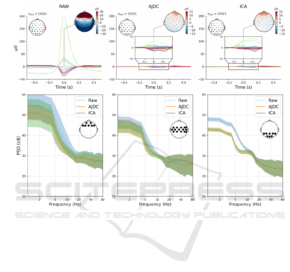
Figure 1: Artefact Reduction. (a) Blink EPs for the conditions: RAW (left), AJDC-corrected (centre), ICA-corrected (right)

signals. The grand average of the EPs across subjects is presented. At the top of each plot, topographies represent the spatial

distribution of the blink EPs at t = 0 s corresponding to the blink peak. The inset boxes zoom in on the corrected EPs for better

visualization of the differences between methods. Vertical axis: amplitude (µV); horizontal axis: time (s). (b) Power spectra

averaged on three scalp regions (from left to right: frontal, central, posterior) and averaged across subjects. Spectra derived

from raw signals are represented in blue, those from AJDC-corrected blink epochs in orange, and those from ICA-corrected

blink epochs in green. The lighter shaded area around each PSD represents the standard deviation across subjectts. Vertical

axis: spectral amplitudes (dB) ; horizontal axis: frequencies (Hz). An inset on each plot shows the electrodes that were

included in each scalp region.

between 1 Hz and 80 Hz, with 0.5 Hz frequency bins.

The wavelet cycles were linearly scaled with

frequency to ensure consistent time-frequency

resolution. Morlet wavelets were chosen for their

optimal trade-off between temporal and spectral

resolution (Bertrand et al., 2000). This approach

ensures precise characterization of both low- and

high-frequency bands while preserving consistent

temporal accuracy across the entire frequency range.

The trials were averaged, and the signal power was

then baseline-corrected using a log-ratio, with each

time point corrected relative to the mean power

during a 2-s fixation period (from t = -3 s to t = -1 s).

Furthermore, to check the preservation of MI

signatures after AJDC relative to ICA correction, we

employed Representational Similarity Analysis

(RSA) (Kriegeskorte et al., 2008) of the topographical

patterns. For each participant, we constructed

dissimilarity matrices from the MI-related

topographical maps after AJDC and after ICA,

respectively, by computing pairwise Euclidean

distances between electrode pairs. The similarity

between these matrices was then assessed using

Spearman’s rank correlation coefficient. By

leveraging RSA – which combines the computation

of dissimilarity matrices and their subsequent

correlation – we quantitatively assessed whether the

topographical structure of MI patterns was

maintained across different correction methods.

Automatic Ocular Artifact Correction in Electroencephalography for Neurofeedback

777

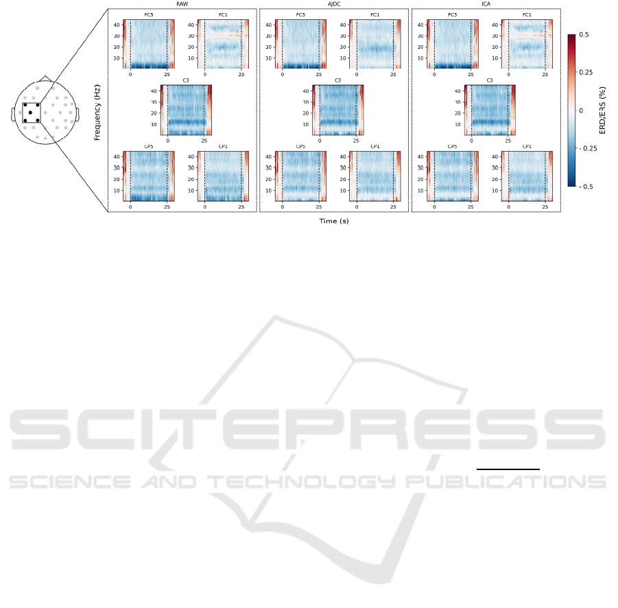
Figure 2: Preservation of MI signatures. Time-frequency representation of EEG power on each electrode of the Laplacian

filter in RAW, AJDC and ICA conditions, during the NF trials. The grand average of the data across subjects is represented.

The thin black dashed lines at 0 and 25 s represent the start and end of NF during the trials. ERD/ERS values are color coded,

with the blue colors representing ERD and the red colors representing ERS. Vertical axis: frequencies (Hz) ; horizontal axis:

time (s).

2.3.3 Simulation of Online Application

To quantify the beta-band (β) activity that participants

aimed to regulate through NF in a pseudo-online

fashion (aka. NF performance), we used the

OpenViBE 2.2.0 (Renard et al., 2010) processing

pipeline applied during the experiment. This pipeline

calculated online β power (online β), during NF trials

and compared it to a reference β power (reference β).

A Laplacian spatial filter was applied to electrode C3

by subtracting signals from adjacent electrodes (CP5,

CP1, FC1, and FC5). The resulting signal was band-

pass filtered between 8 and 30 Hz using an 8

-order

Butterworth filter, then segmented into 1 s epochs

with a 0.75 s overlap. For each epoch, β power was

calculated by squaring and averaging the signal.

Online β was derived by averaging β power values

over the 4 epochs preceding each feedback cycle

during the NF runs (see Dussard et al., 2024 for

details). It was compared to a common reference β

power value derived from a 60 s baseline period

recorded before the NF task. This reference β was

calculated by averaging the median β power of the

AJDC-corrected baseline period and the median β

power of the RAW baseline period.

NF performance was then computed as follows.

Each trial included 16 feedback cycles based on 16

online β values, which were compared to the

participant’s reference β. We divided each online β

value by the reference β and computed the median of

these 80 ratios (16 values per trial × 5 trials per run)

for every NF run. The result was log-transformed,

with the sign inverted, so that positive values

indicated a reduction in online β relative to reference

β, thus reflecting successful NF performance.

Finally, since AJDC was calibrated at the

beginning of the experiment and applied throughout

the NF runs, we also examined the quality of the

correction over time. To do this, we extracted a

signal-to-noise ratio (SNR) of the blink EPs,

calculated across the NF runs as follows:

𝑆𝑁𝑅 = −10log

𝑠𝑖𝑔𝑛𝑎𝑙



𝑠𝑖𝑔𝑛𝑎𝑙





(6)

2.3.4 Statistical Analyses

(1) For artifact reduction analysis, PSD values of

blink epochs on each electrode and at each frequency

(1 to 80 Hz) were compared between ICA and AJDC

corrections.

(2) For MI-related signature preservation analysis,

power in the frequency band and electrodes of interest

(that is, 8-30 Hz band on FC1, FC5, C3, CP1, and

CP5) was averaged and compared 2-by-2 between the

RAW, AJDC, and ICA conditions.

(3) For SNR analysis, SNR values on each electrode

were compared between the first and last NF runs,

which were separated by an interval of 15-20 minutes.

When relevant, normality was assessed with the

Shapiro-Wilk test. When normality was met, paired t-

tests across subjects were used; otherwise, we used

Wilcoxon signed-rank tests. For each analysis, the p-

values were corrected for multiple comparisons using

the False Discovery Rate (FDR) correction from

Benjamini-Hochberg (Benjamini & Hochberg, 1995),

with FDR-corrected significance level (pFDR) set at

0.05.

BIOSIGNALS 2025 - 18th International Conference on Bio-inspired Systems and Signal Processing

778

3 RESULTS

3.1 Artifact Reduction

We first investigated the artifact reduction resulting

from AJDC and ICA. For this purpose, we compared

the blink EPs averaged from RAW signals and from

signals corrected by AJDC and ICA. (see Figure 1.a).

Both correction methods visibly reduced blink

artifacts, as shown in the topographies at t = 0 s

corresponding to the peak of the blink artifact, though

some

rontal activity remained present in the

corrected signals. Focusing on frontal electrodes

(Fp1, Fp2, F7, F3, Fz, F4, F8), the average artifact

amplitude reduction was of 75.88 µV (± 24.28 µV;

[mean ± SD]) for AJDC and 75.56 µV (± 23.49 µV;

[mean ± SD]) for ICA. The differences between

AJDC and ICA seemed minimal, with only slight

variations in the spatial distribution and intensity of

residual activity.

To further investigate the effects of AJDC and ICA

on artifact reduction, we analyzed the PSD averaged

from blink epochs across frontal, central, and

posterior regions for both raw and corrected signals

(see Figure 1.b). A slight divergence between AJDC-

and ICA-corrected PSDs emerged only in the frontal

region, particularly at frequencies above 10 Hz.

However, AJDC- and ICA- corrected PSDs did not

show any significant difference on either electrode or

frequency (all pFDR > 0.05).

3.2 Preservation of MI Signatures

We investigated the extent to which the AJDC

preserved neurophysiological information of interest

despite the ocular artifact removal. Figure 2 shows the

time-frequency representation of the targeted beta

ERD during the NF trials, across the electrodes

involved in the Laplacian filter (that was used during

the NF protocol, see Methods). Both correction

methods appeared to preserve a similar MI-related

signature, except for electrode FC1 were a high-

frequency activity (around 30 Hz) was present in

RAW and ICA-corrected data but absent in AJDC-

corrected data. Some weak differences between

AJDC- and ICA-corrected time-frequency

representations were also visible in the low-frequency

range (<5 Hz) on CP1. Yet, the comparison of the

mean ERD in the beta band (8-30 Hz) between 0 and

25 s on the five-electrode involved in the Laplacian

computation did not show any statistically significant

2-by-2 difference between RAW, AJDC-corrected

and ICA-corrected data (pFDR > 0.05).

Furthermore, RSA analysis revealed a mean

similarity score of 0.87 ± 0.07 ([mean ± SD]),

indicating a preservation of the topographical

structure of MI patterns across the AJDC and ICA

correction methods.

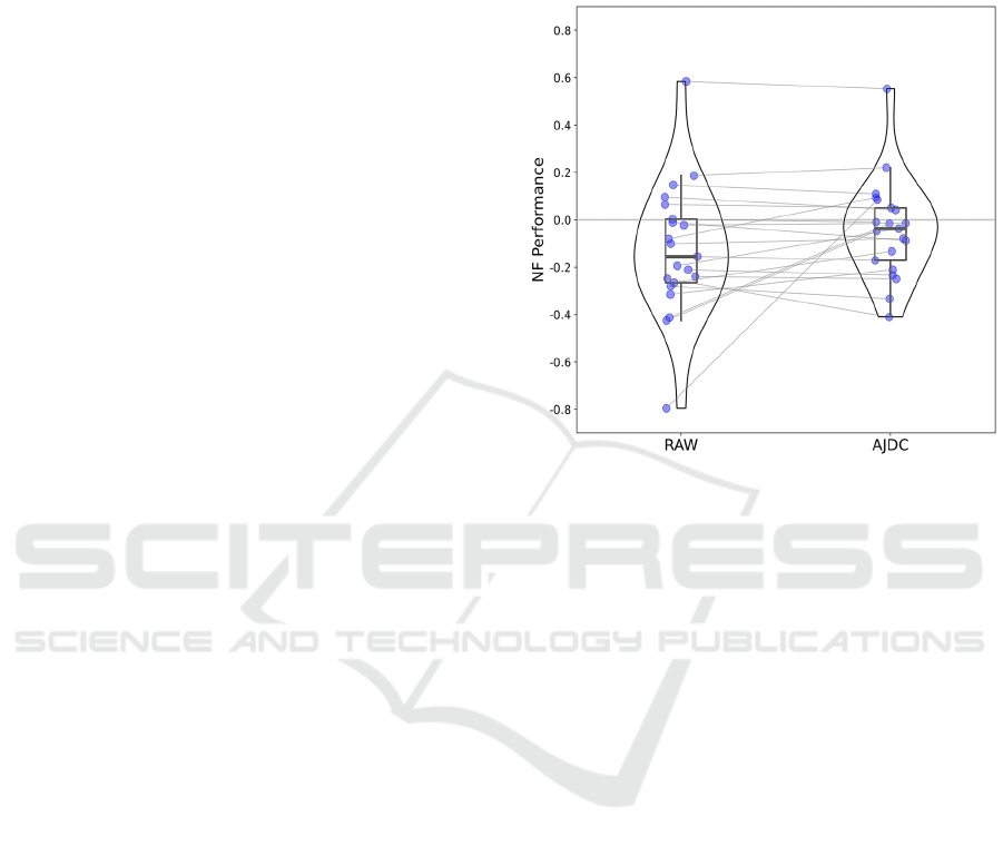
Figure 3: Comparison of NF performance between RAW

and AJDC conditions. Blue dots represent individual data.

For each condition, the thick horizontal black line is the

median value across subjects, the box plot corresponds to

the second and third quartiles, and the vertical these black

lines correspond to the lower and upper quartiles (excluding

outlier values). Violin plots of the individual data are also

included. Vertical axis: NF performance; horizontal axis:

conditions.

3.3 Simulation of Online Application

We evaluated the potential impact of AJDC on NF

performance in a pseudo-online framework,

replaying the data in real-time in OpenVibe to

simulate live recording conditions. Analysis of RAW

versus AJDC-corrected neurofeedback performance

showed no significant effect, with pFDR > 0.05.

Moreover, to evaluate the consistency of

the AJDC correction over time, we compared

SNR values between the first and last NF runs (see

Figure 4). A general decrease in SNR was observed

across electrodes, with lower SNR values in the last

run compared to the first one. Statistical analysis

revealed significant SNR differences on three

electrodes (F3, F8 and FC5; pFDR < 0.05). However,

this did not seem to impact NF performance insofar

as there was no significant difference between the

delta of NF performance between AJDC and RAW in

the first run and the delta of NF performance between

AJDC and RAW in the last run (pFDR > 0.05).

Automatic Ocular Artifact Correction in Electroencephalography for Neurofeedback

779

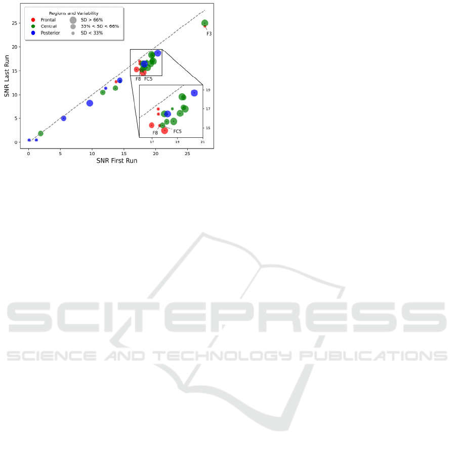
Figure 4: Difference in SNR between the first and last NF

runs for each electrode. The electrodes are colored

according to their scalp region: frontal (red), central

(green), and posterior (blue), corresponding to the same

regions as in Figure 2. The size of the colored circle reflects

the variability (standard deviation, SD) of the first vs. last

run SNR difference across subjects. For visualization

purpose, 3 circle size are represented: the larger circles

represent the electrodes with a SD of SNR difference

belonging to the 66% higher percentile of all SD values

across electrodes, the medium size circles represent the

electrodes with a SD value between 33% and 66% of all SD

values, and smaller circles represent electrodes with a SD

less than 33% of all SD values.

4 DISCUSSION

In NF and BCI, ocular artifacts – particularly those

from eye blinks – present a substantial challenge, as

they can severely distort EEG signatures. This study

evaluated the efficacy of the AJDC method for

automatic blink artifact correction in EEG data,

benchmarking it against the well-known ICA.

Our study showed that AJDC effectively reduces

blink artifacts in EEG signals, notably by attenuating

the frontal blink-related activity, which often disrupts

BCI and NF applications (Jiang et al., 2019). This

result aligns with expectations, as blink artifacts are

known to predominantly impact frontal channels due

to their proximity to the ocular sources (Joyce et al.,

2004). Although both AJDC and ICA methods

offered comparable performance, minor differences

appeared in high frequencies (>10 Hz) in the frontal

regions, where AJDC exhibited a correction profile

distinct from ICA. In the PSD analysis, the mean PSD

across scalp regions and subjects was lower for AJDC

compared to ICA; ICA PSD was closer to the RAW

PSD. This slight variation may reflect specific

characteristics of the AJDC decomposition process,

potentially influencing the spectral content (Congedo

et al., 2008). Although these differences did not reach

statistical significance, they may reflect unique

characteristics of AJDC correction. These

observations align with the conclusions of

Barthélemy et al., 2017, who demonstrated that

AJDC can effectively isolate and reduce ocular

artifacts. They also found minor differences between

manual denoising by ICA and automatic denoising by

AJDC in the PSD of frontal electrodes, suggesting

that AJDC may offer a distinct profile in terms of

power distribution in this region.

Beyond artifact reduction, we also considered the

AJDC method’s ability to preserve essential

neurophysiological information of interest, that is,

here, ERD in the beta band. In this regard, AJDC

seemed to preserve MI-related activity within the 8-

30 Hz band; there was no evidence of signal

deformation in this frequency range (see Figure 2).

This observation is in line with the findings from

Barthélemy et al., 2017, who demonstrated that

event-related potentials (ERPs) remained unaffected

by distortions from AJDC correction, supporting its

suitability for preserving key neural signals. That

said, some difference was observed around 30Hz on

electrode FC1. We went back to individual data and

noted that this difference was attributable to a single

subject who exhibited a high fluctuation in EEG

activity at this frequency. This fluctuation was absent

in the AJDC calibration data and therefore picked up

to some extent in the ocular component targeted for

removal during the NF runs. This outcome suggests

that while AJDC is robust in most cases, subject-

specific EEG variations or outliers may lead to

unanticipated inclusions in the correction process.

This is further supported by the RSA scores, which

indicated an average similarity above 85%. While this

represents a high degree of similarity, it is not perfect

(i.e., not 100%), suggesting the presence of residual

differences. Such variations can influence the motor

signature by introducing unintended corrections. This

observation resonates with findings from prior

studies, which emphasized the challenges posed by

intra-subject variability in EEG and artifact

correction methods (Ronca et al., 2024; Wei et al.,

2021).

In terms of NF performance, no significant

difference was found between the RAW and AJDC-

corrected conditions in a pseudo-online framework,

where data were replayed in real-time in OpenVibe to

simulate live recording conditions (see Figure 3). For

the purpose of this analysis, a common reference β

power was used for both methods, calculated as the

mean of the reference β power from each method.

BIOSIGNALS 2025 - 18th International Conference on Bio-inspired Systems and Signal Processing

780

However, we checked that a method-specific

reference β did not alter our conclusions. This is

consistent with the findings of Dussard et al., 2024,

who demonstrated that Laplacian techniques are

resilient to ocular artifacts. It is however worth noting

that more complex spatial filtering methods that

integrate information from the entire scalp, such as

Common Spatial Patterns (CSP) (Blankertz et al.,

2008), are more sensitive to ocular artifacts,

potentially impacting their performance. CSPs are

commonly used in BCI protocols due to their

effectiveness in discriminating MI-related EEG

patterns, yet they are sensitive to ocular artifacts that

can degrade their accuracy if not adequately managed

(Jafarifarmand & Badamchizadeh, 2019). AJDC may

be particularly useful in the context of CSP and other

advanced feature extraction methods.

In addition to the overall performance analysis, a

notable aspect of our results is the observed

progressive decline in the effectiveness of AJDC

correction over the course of the experiment (see

Figure 4). This trend suggests that periodic

adjustments or recalibrations may be necessary to

sustain the AJDC method efficacy. This temporal

degradation likely arises from dynamic changes in

artifact characteristics and neural signal properties

(Ambrogioni et al., 2017; Islam et al., 2021). This

observation is in agreement with broader findings in

the literature on BCI and NF systems, where

maintaining stable performance across time is often

challenging due to various sources of signal

variability, including changes in electrode

impedance, user fatigue, and cognitive state

fluctuations (Alkoby et al., 2018; Saha & Baumert,

2020; Vidaurre & Blankertz, 2010). Such fluctuations

can impact the consistency of the neural signals,

thereby complicating real-time processing and

artifact correction. An improvement to the AJDC

method could involve implementing a real-time,

offset calibration, where a new correction matrix is

recalculated in the background during real-time

artifact correction.

While the AJDC method shows promising results

in blink artifact correction, certain limitations remain.

First, AJDC requires manual identification of artifacts

components, a step conducted at the beginning of the

experiment in our protocol. While this initial

calibration minimizes variability, it relies on expert

input, which introduces inter-operator variability and

limits reproducibility across different experimental

setups (Barthélemy et al., 2017). Additionally,

although our study focused solely on blink artifacts, a

multitude of other artifact types – including

physiological (e.g. muscle activity) and

environmental noise – can significantly impact EEG

signals (Tatum et al., 2011). The efficacy of AJDC

for these types of artifacts has yet to be assessed

comprehensively, as various studies highlight the

importance of robust correction methods for diverse

EEG artifacts to ensure signal integrity in BCI

applications (McDermott et al., 2022).

Another limitation is the offline nature of our

comparison. While this approach was justified by the

shared BSS framework of both AJDC and ICA

methods, it would be interesting to also test AJDC

against a real-time method, such as ASR (Mullen et

al., 2015), for a fuller methodological benchmark.

This comparison is particularly relevant for BCI and

NF applications, where continuous adaptation and

real-time processing are critical (Saha & Baumert,

2020). Our comparison with ICA is valuable given

the well-documented strengths and limitations of ICA

in artifact correction. Another interesting suggestion

could be to test AJDC on clean EEG data artificially

contaminated with controlled artifacts (Chavez et al.,

2018). This approach would allow for a rigorous

evaluation of AJDC artifact correction efficacy and

its impact on neural signals. Furthermore, such a

setup would enable the exploration of additional

metrics, such as phase delay, relative root mean

square error, coherence or Riemannian distance.

These measures could provide complementary

insights into the quality of artifact correction.

Finally, this study serves as a proof of concept,

demonstrating the potential of the AJDC method in

comparison to ICA using data from healthy subjects.

However, to fully assess the robustness and clinical

applicability of AJDC, it would be essential to

evaluate its performance on patients’ data. Patients’

populations may exhibit more pronounced artifacts

due to various factors such as increased physiological

variability, medication effects, or underlying

neurological conditions (Karson, 1983; Kimura et al.,

2017). Evaluating AJDC on such data would provide

critical insights into its efficacy in real-world clinical

contexts.

In summary, our study offers a promising first

step toward robust real-time EEG artifact correction

with AJDC, highlighting areas for further

development in automating and validating the method

across diverse recording conditions and artifact types.

REFERENCES

Alkoby, O., Abu-Rmileh, A., Shriki, O., & Todder, D.

(2018). Can We Predict Who Will Respond to

Neurofeedback? A Review of the Inefficacy Problem

Automatic Ocular Artifact Correction in Electroencephalography for Neurofeedback

781

and Existing Predictors for Successful EEG

Neurofeedback Learning. Neuroscience, 378, 155–164.

Al-Quraishi, M. S., Elamvazuthi, I., Daud, S. A.,

Parasuraman, S., & Borboni, A. (2018). EEG-Based

Control for Upper and Lower Limb Exoskeletons and

Prostheses: A Systematic Review. Sensors (Basel,

Switzerland), 18, 3342.

Ambrogioni, L., Gerven, M. A. J. van, & Maris, E. (2017).

Dynamic decomposition of spatiotemporal neural

signals. PLOS Computational Biology, 13(5).

Barachant, A., Barthélemy, Q., Wagner vom Berg, G.,

Gramfort, A., King, J.-R., & Rodrigues, P. L. C. (2024).

pyRiemann/pyRiemann: V0.6 (Version v0.6)

[Computer software].

Barthélemy, Q., Mayaud, L., Renard, Y., Kim, D., Kang,

S.-W., Gunkelman, J., & Congedo, M. (2017). Online

denoising of eye-blinks in electroencephalography.

Clinical Neurophysiology, 47(5–6), 371–391.

Benjamini, Y., & Hochberg, Y. (1995). Controlling the

False Discovery Rate: A Practical and Powerful

Approach to Multiple Testing. Journal of the Royal

Statistical Society: Series B (Methodological), 57(1),

289–300.

Bertrand, O., Tallon-Baudry, C., & Pernier, J. (2000). Time-

Frequency Analysis of Oscillatory Gamma-Band

Activity: Wavelet Approach and Phase-Locking

Estimation (Vol. 2, pp. 919–922).

Blankertz, B., Tomioka, R., Lemm, S., Kawanabe, M., &

Muller, K. (2008). Optimizing Spatial filters for Robust

EEG Single-Trial Analysis. IEEE Signal Processing

Magazine, 25(1), 41–56.

Chavez, M., Grosselin, F., Bussalb, A., De Vico Fallani, F.,

& Navarro-Sune, X. (2018). Surrogate-Based Artifact

Removal From Single-Channel EEG. IEEE

Transactions on Neural Systems and Rehabilitation

Engineering, 26(3), 540–550.

Congedo, M., Gouy-Pailler, C., & Jutten, C. (2008). On the

blind source separation of human electroencephalo-

gram by approximate joint diagonalization of second

order statistics. Clinical Neurophysiology, 119(12),

2677–2686.

Croft, R. J., & Barry, R. J. (2000). EOG correction of blinks

with saccade coefficients: A test and revision of the

aligned-artefact average solution. Clinical

Neurophysiology, 111(3), 444–451.

Delorme, A., Sejnowski, T., & Makeig, S. (2007).

Enhanced detection of artifacts in EEG data using

higher-order statistics and independent component

analysis. NeuroImage, 34(4), 1443–1449.

Dussard, C., Pillette, L., Dumas, C., Pierrieau, E.,

Hugueville, L., Lau, B., Jeunet-Kelway, C., & George,

N. (2024). Influence of feedback transparency on motor

imagery neurofeedback performance: The contribution

of agency. Journal of Neural Engineering, 21(5).

Friedman, D., Claassen, J., & Hirsch, L. J. (2009).

Continuous electroencephalogram monitoring in the

intensive care unit. Anesthesia and Analgesia, 109(2),

506–523.

Gramfort, A., Luessi, M., Larson, E., Engemann, D. A.,

Strohmeier, D., Brodbeck, C., Parkkonen, L., &

Hämäläinen, M. S. (2014). MNE software for

processing MEG and EEG data. NeuroImage, 86, 446–

460.

Hagemann, D., & Naumann, E. (2001). The effects of

ocular artifacts on (lateralized) broadband power in the

EEG. Clinical Neurophysiology, 112(2), 215–231.

Islam, Md. K., Rastegarnia, A., & Sanei, S. (2021). Signal

Artifacts and Techniques for Artifacts and Noise

Removal. In Signal Processing Techniques for

Computational Health Informatics (Vol. 192, pp. 23–

79). Springer.

Iwasaki, M., Kellinghaus, C., Alexopoulos, A. V., Burgess,

R. C., Kumar, A. N., Han, Y. H., Lüders, H. O., &

Leigh, R. J. (2005). Effects of eyelid closure, blinks,

and eye movements on the electroencephalogram.

Clinical Neurophysiology, 116(4), 878–885.

Jafarifarmand, A., & Badamchizadeh, M. A. (2019). EEG

Artifacts Handling in a Real Practical Brain–Computer

Interface Controlled Vehicle. IEEE Transactions on

Neural Systems and Rehabilitation Engineering, 27(6),

1200–1208.

Jiang, X., Bian, G.-B., & Tian, Z. (2019). Removal of

Artifacts from EEG Signals: A Review. Sensors (Basel,

Switzerland), 19(5), 987.

Joyce, C. A., Gorodnitsky, I. F., & Kutas, M. (2004).

Automatic removal of eye movement and blink artifacts

from EEG data using blind component separation.

Psychophysiology, 41(2), 313–325.

Karson, C. N. (1983). Spontaneous Eye-Blinks Rates and

Dopaminergic Systems. Brain, 106(3), 643–653.

Kimura, N., Watanabe, A., Suzuki, K., Toyoda, H.,

Hakamata, N., Fukuoka, H., Washimi, Y., Arahata, Y.,

Takeda, A., Kondo, M., Mizuno, T., & Kinoshita, S.

(2017). Measurement of spontaneous blinks in patients

with Parkinson’s disease using a new high-speed blink

analysis system. Journal of the Neurological Sciences,

380, 200–204.

Kriegeskorte, N., Mur, M., & Bandettini, P. A. (2008).

Representational similarity analysis—Connecting the

branches of systems neuroscience. Frontiers in Systems

Neuroscience, 2

Langlois, D., Chartier, S., & Gosselin, D. (2010). An

Introduction to Independent Component Analysis:

InfoMax and FastICA algorithms. Tutorials in

Quantitative Methods for Psychology, 6(1), 31–38.

Larson, E., Gramfort, A., Engemann, D. A., Leppakangas,

J., Brodbeck, C., Jas, M., Brooks, T. L., Sassenhagen,

J., McCloy, D., Luessi, M., King, J.-R., Höchenberger,

R., Goj, R., Favelier, G., Brunner, C., van Vliet, M.,

Wronkiewicz, M., Rockhill, A., Holdgraf, C., …

luzpaz. (2024). MNE-Python (Version v1.8.0)

[Computer software].

Lotte, F., Bougrain, L., & Clerc, M. (2015).

Electroencephalography (EEG)‐Based Brain–

Computer Interfaces. In J. G. Webster (Ed.), Wiley

Encyclopedia of Electrical and Electronics

Engineering (1st ed., p. 44). Wiley.

Makeig, S., Bell, A., Jung, T.-P., & Sejnowski, T. (1996).

Independent Component Analysis of Electroencephalo-

BIOSIGNALS 2025 - 18th International Conference on Bio-inspired Systems and Signal Processing

782

graphic Data. Advances in Neural Information

Processing Systems, 8.

McDermott, E. J., Raggam, P., Kirsch, S., Belardinelli, P.,

Ziemann, U., & Zrenner, C. (2022). Artifacts in EEG-

Based BCI Therapies: Friend or Foe? Sensors, 22(1),

96.

Mullen, T. R., Kothe, C. A. E., Chi, Y. M., Ojeda, A., Kerth,

T., Makeig, S., Jung, T.-P., & Cauwenberghs, G.

(2015). Real-Time Neuroimaging and Cognitive

Monitoring Using Wearable Dry EEG. IEEE

Transactions on Bio-Medical Engineering, 62(11),

2553–2567.

Mumtaz, W., Rasheed, S., & Irfan, A. (2021). Review of

challenges associated with the EEG artifact removal

methods. Biomedical Signal Processing and Control,

68, 102741.

Omejc, N., Rojc, B., Battaglini, P. P., & Marusic, U. (2019).

Review of the therapeutic neurofeedback method using

electroencephalography: EEG Neurofeedback. Bosnian

Journal of Basic Medical Sciences, 19(3), 213–220.

Pfurtscheller, G., & Lopes da Silva, F. H. (1999). Event-

related EEG/MEG synchronization and desynchroniza-

tion: Basic principles. Clinical Neurophysiology,

110(11), 1842–1857.

Renard, Y., Lotte, F., Gibert, G., Congedo, M., Maby, E.,

Delannoy, V., Bertrand, O., & Lécuyer, A. (2010).

OpenViBE: An Open-Source Software Platform to

Design, Test, and Use Brain–Computer Interfaces in

Real and Virtual Environments. Presence, 19(1), 35–

53.

Ronca, V., Capotorto, R., Di Flumeri, G., Giorgi, A., Vozzi,

A., Germano, D., Virgilio, V. D., Borghini, G.,

Cartocci, G., Rossi, D., Inguscio, B. M. S., Babiloni, F.,

& Aricò, P. (2024). Optimizing EEG Signal Integrity:

A Comprehensive Guide to Ocular Artifact Correction.

Bioengineering, 11(10), 1018.

Saha, S., & Baumert, M. (2020). Intra- and Inter-subject

Variability in EEG-Based Sensorimotor Brain

Computer Interface: A Review. Frontiers in

Computational Neuroscience, 13, 87.

Tatum, W. O., Dworetzky, B. A., & Schomer, D. L. (2011).

Artifact and Recording Concepts in EEG. Journal of

Clinical Neurophysiology, 28(3), 252–263.

Thomas, J., Thangavel, P., Peh, W. Y., Jing, J., Yuvaraj, R.,

Cash, S. S., Chaudhari, R., Karia, S., Rathakrishnan, R.,

Saini, V., Shah, N., Srivastava, R., Tan, Y.-L.,

Westover, B., & Dauwels, J. (2021). Automated Adult

Epilepsy Diagnostic Tool Based on Interictal Scalp

Electroencephalogram Characteristics: A Six-Center

Study. International Journal of Neural Systems, 31(5),

2050074.

Vidaurre, C., & Blankertz, B. (2010). Towards a Cure for

BCI Illiteracy. Brain Topography, 23(2), 194–198.

Wei, C.-S., Keller, C. J., Li, J., Lin, Y.-P., Nakanishi, M.,

Wagner, J., Wu, W., Zhang, Y., & Jung, T.-P. (2021).

Editorial: Inter- and Intra-subject Variability in Brain

Imaging and Decoding. Frontiers in Computational

Neuroscience, 15, 791129.

Zikov, T., Bibian, S., Dumont, G. A., Huzmezan, M., &

Ries, C. R. (2002). A wavelet based de-noising

technique for ocular artifact correction of the

electroencephalogram. 24th Annual Conference of the

Biomedical Engineering Society, 1, 98–105 vol.1.

Automatic Ocular Artifact Correction in Electroencephalography for Neurofeedback

783