Zeroth Order Optimization for Pretraining Language Models

Nathan Allaire

1 a

, Mahsa Ghazvini Nejad

, S

ebastien Le Digabel

1 b

and Vahid Partovi Nia

2 c

GERAD, Polytechnique Montr

eal, Montr

eal, Canada

Noah’s Ark Lab, Montr

eal, Canada

Keywords:

Backpropagation, Deep Learning, Language Models, Stochastic Gradient Descent, Transformer Architecture,

Pretraining.

Abstract:

The physical memory for training Large Language Models (LLMs) grow with the model size, and are limited

to the GPU memory. In particular, back-propagation that requires the computation of the ﬁrst-order derivatives

adds to this memory overhead. Training extremely large language models with memory-efﬁcient algorithms

is still a challenge with theoretical and practical implications. Back-propagation-free training algorithms,

also known as zeroth-order methods, are recently examined to address this challenge. Their usefulness has

been proven in ﬁne-tuning of language models. However, so far, there has been no study for language model

pretraining using zeroth-order optimization, where the memory constraint is manifested more severely. We

build the connection between the second order, the ﬁrst order, and the zeroth order theoretically. Then, we

apply the zeroth order optimization to pre-training light-weight language models, and discuss why they cannot

be readily applied. We show in particular that the curse of dimensionality is the main obstacle, and pave the

way towards modiﬁcations of zeroth order methods for pre-training such models.

1 INTRODUCTION

For the past decades, ﬁrst order (FO) optimiza-

tion has been the preferred choice in the machine

learning community. Stochastic gradient descent

(SGD) (Amari, 1993) was introduced as an efﬁ-

cient and robust method for training and ﬁne-tuning

language models (LM). Later, the Adam optimizer

(Kingma, 2014) and its variants (Loshchilov and Hut-

ter, 2017) have been a major improvement for those

tasks by adding momentum and adaptive learning

rate to SGD. However, second order (SO) optimiza-

tion is less common than FO methods such as SGD

and Adam in machine learning community due to its

higher computational and memory costs. The SO op-

timization adds some precious information and often

yields a faster convergence than FO (Shepherd, 2012)

it is still under progress for training deep learning

models.

Recently, researchers have shown that larger mod-

els lead to a smaller loss value and therefore lead to a

more accurate model (Kaplan et al., 2020). In return,

LLMs continue to grow in size and complexity, and

https://orcid.org/0009-0006-0694-8216

https://orcid.org/0000-0003-3148-5090

https://orcid.org/0000-0001-6673-4224

the memory constraints imposed by traditional train-

ing methods present a signiﬁcant hurdle. Since the in-

troduction of the BERT model (Vaswani et al., 2017)

common language models have grown from 340M to

70B ∼ 200× while the GPU memories have grown

from 16GB to 80GB almost 5×. Moreover, (Malladi

et al., 2023) showed that the back-propagation of the

OPT-13B model requires 12× more memory than in-

ference. Those observations prompted a reevaluation

of approaches for more resource-efﬁcient learning,

specially targeting training, pre-training, and ﬁne-

tuning.

Zeroth-order (ZO) methods includes derivative-

free optimization methods also known as black box

optimization. However, in the machine learning com-

munity it is referred to the algorithms that approxi-

mate the full gradient via gradient estimators based

only on the function evaluation in the forward pass

(Blum, 1954), (Spall, 1992). In the context of ma-

chine learning, ZO methods do not need to back-

propagate and therefore, cut the memory required

in training step. Back-propagation-free methods

for ﬁne-tuning LLMs were ﬁrst introduced in (Mal-

ladi et al., 2023) that unveils the ﬁrst Memory efﬁ-

cient Zeroth-Order algorithm. Several extensions and

variants of this algorithm were disclosed in (Gau-

Allaire, N., Ghazvini Nejad, M., Le Digabel, S. and Partovi Nia, V.

Zeroth Order Optimization for Pretraining Language Models.

DOI: 10.5220/0013261100003905

Paper published under CC license (CC BY-NC-ND 4.0)

In Proceedings of the 14th International Conference on Pattern Recognition Applications and Methods (ICPRAM 2025), pages 113-121

ISBN: 978-989-758-730-6; ISSN: 2184-4313

113

tam et al., 2024), and historically initiated in (Liu

et al., 2018) to develop memory efﬁcient zeroth or-

der stochastic variance reduction of the gradient to

tackle the high-variance issue inherent to ZO. Re-

cently, (Zhang et al., 2024) proposed a benchmark on

ZO methods and showed their efﬁciency on several

ﬁne-tuning tasks. We observed that that the variance

inﬂation in zeroth order training is rather a blessing.

All these works focus on ﬁne-tuning of a language

model and avoid addressing the more complex pre-

training step. We dive into the largely unexplored

ﬁeld of ZO optimization for pre-training focusing on

the following question: can language models be effec-

tively pre-trained using ZO optimization, and if not,

what are the underlying limitations and how can they

be overcome?

To answer this question ﬁrst we try to understand

the relationship between second order, ﬁrst order, and

zero order using simple but insightful theory. Then we

aim to focus on two key model characteristics: the di-

mension of the problem and the variance associated to

ZO optimization in language model pretraining. We

establish our experiments using a light-weight 20M

transformer model due to lack of computational re-

sources. However, we expect a similar behaviour for

light-weight language models under 1B parameters.

The behaviour of model pretraining changes often

after surpassing billion parameters, see for instance

(Zeng et al., 2023).

Our main contributions include

• We make a brief overview of the main (SO, FO,

ZO) optimization methods and disclose several

theoretical results on the optimal value of the

learning rate to establish a concrete connection

between SO and FO in particular,

• We pre-train the Llama2 20M model with vanilla

FO and ZO optimization and showcase the efﬁc-

tiveness of ZO methods in this context,

• Run several experiments on a controlled ZO gra-

dient variance, and demonstrate that the high vari-

ance of ZO is needed for pre-training light weight

language models.

2 OPTIMIZATION

BACKGROUND

Consider the unconstrained optimization problem

min

θ∈R

L(θ), L(θ) =

∑

i=1

(θ), (1)

where L : R

→R is a non-convex loss function, each

is the loss of a single training instance. This opti-

mization problem encapsulates most of deep learning

training problems, including LLMs pretraining and

ﬁne-tuning.

2.1 Second Order

Optimization is a fundamental aspect of various sci-

entiﬁc and engineering disciplines, where the goal is

to ﬁnd the best parameter setting from a set of feasi-

ble solutions. While FO optimization methods, such

as gradient descent, are widely used in deep learning

training thanks to their simplicity and efﬁciency, they

often struggle with issues like slow convergence and

sensitivity to the choice of the step size, learning rate,

etc. SO optimization techniques leverage not only the

gradient (ﬁrst derivative) but also the Hessian matrix

(second derivative) of the objective function. By in-

corporating the curvature information, these methods

provide a more accurate descent and a faster conver-

gence to the minimum.

One of the most prominent SO optimization meth-

ods is Newton’s method. Newton’s method uses both

the gradient and the Hessian matrix to iteratively ﬁnd

the stationary points of a function, by assuming an

approximate quadratic function over the loss L. This

is a common assumption in neural networks near the

minimum

L(θ) ≈

⊤

Hθ + g

⊤

θ, (2)

where {∇

L}= H is the n ×n Hessian and ∇L = g is

the gradient vector of size n. In general, the Newton

update provides potential candidates for local min-

ima, but gives an exact minima in a single update if

the function is quadratic and has a unique minimum,

i.e. has a positive deﬁnite Hessian. The update rule

for Newton’s method is given by

k+1

= θ

−H

−1

g, (3)

where θ

is the current update, g = ∇L(θ

) is the gra-

dient, and H = ∇

L(θ

) is the Hessian, both evalu-

ated at θ

. The Newton’s method achieves quadratic

convergence near the optimal solution, making it sig-

niﬁcantly faster than FO methods for approximately

quadratic functions. However, in deep learning appli-

cations, applying the Newton’s method is challeng-

ing, e.g. the computational cost of calculating and in-

verting the n ×n Hessian matrix, especially for high-

dimensional problems with a large n such as large

language models. In deep learning practice, the sec-

ond order algorithms approximate the Hessian using

the squared gradient, i.e. H ≈ gg

⊤

. This approxima-

tion has originated from the Fisher information iden-

tity, where the second derivative of the negative log-

likelihood equals the gradient square in expectation

(Lehmann and Casella, 1998).

ICPRAM 2025 - 14th International Conference on Pattern Recognition Applications and Methods

114

Figure 1: The Newton’s method (red) compared with FO

gradient descent (blue) and its stochastic variant (green).

2.2 First Order

One of the most widely used FO optimization meth-

ods is the gradient descent. The main idea behind the

gradient descent is to iteratively move in the direction

of the steepest descent, which is determined by the

negative gradient of the function. The update rule for

gradient descent is given by

k+1

= θ

−ηg, (4)

where η is a positive learning rate. This formulation

surprisingly resembles (3). Hereafter, we aim to pro-

vide a clearer connection between SO and FO meth-

ods using a theoretical study on the learning rate. The

learning rate is widely studied in the literature with

established theoretical results under different assump-

tions for L, see for instance (Prazeres and Oberman,

2021; Wu et al., 2018)

The gradient step in (4) equals the Newton step (3)

for a diagonal Hessian with constant positive diagonal

elements h

= η

−1

, ∀i ∈ {1, . . . , n}, see Figure 1. FO

methods like gradient descent (GD) typically exhibit

linear convergence, meaning the error decreases pro-

portionally to the current error at each step. In con-

trast, Newton’s method often achieves quadratic con-

vergence near the optimal solution. In other words,

the error decreases proportionally to the square of

the current error, leading to much faster convergence

when the step is taken close to the minimum.

The optimal learning rate is rarely studied in

practice, however it is not difﬁcult to derive it in a

quadratic problem. Note that the Newton’s method

moves to the minimum in a single iteration irrespec-

tive of the initial value. A quadratic problem is often

formulated as

Q (θ) =

⊤

Aθ + b

⊤

θ,

where A is the matrix composed of the quadratic

weights, and b is the linear component. We use

align this notations with (2), and assume Q ≡

L is a

quadratic approximation of a deep learning loss L for

simplicity. Therefore, given a positive-deﬁnite Hes-

sian, and a vector of gradients g the minimum of the

quadratic approximation is attained at θ

∗

= −H

−1

Lemma 1. Assume the quadratic problem

L(θ) = θ

⊤

Hθ + g

⊤

θ,

with a positive constant diagonal Hessian H = λI,

where I is the identity matrix. The gradient descent

attains the minimum with the optimal learning rate

η =

Proof. The proof is straightforward by assuring that

the loss function attains its minimum in a single up-

date, i.e. θ

t+1

−θ

= −ηg = θ

∗

= −H

−1

g. Given

H = λI, the gradient descent updates reaches to the

minimum in a single step if ηg =

g, equivalently

η =

A constant diagonal Hessian is too restrictive, and

a more general result can be developed.

Theorem 1. Suppose the quadratic problem

L(θ) =

⊤

Hθ + g

⊤

θ,

with a diagonal Hessian H = diag(h

) where diag

produces a diagonal matrix with h

> 0, as their main

diagonal elements. The optimal learning rate is

∗

∑

i=1

∑

i=1

where g is the gradient vector, i.e.

∗

∑

i=1

(∇

∑

i=1

(∇

Proof. The approach in Lemma 1 that matches the

Newton update with the gradient descent is an under-

speciﬁed vector equation, and cumbersome to solve.

Therefore, we directly minimize the loss in a single

update, i.e. minimizing

L(θ

t+1

−θ

) in terms of η

G(η) =

L(θ

t+1

−θ

) =

⊤

Hg −ηg

⊤

With G a quadratic univariate function minimized at

∗

⊤

. Given that H is diagonal, the optimal

learning rate simpliﬁes to

∗

∑

i=1

∑

i=1

Zeroth Order Optimization for Pretraining Language Models

115

In high-dimensional settings such as deep learning

loss optimization, the Hessian is highly non-diagonal,

and the learning rate is usually tuned in practice by

running several experiments. It is more important to

specify a range in a general case.

Theorem 2. Assume the quadratic problem

L(θ) = θ

⊤

Hθ + g

⊤

θ,

with a positive deﬁnite Hessian. The optimal learn-

ing lies within the range

max

≤ η

∗

≤

min

where

max

, λ

min

are the largest and smallest eigenvalues of

the Hessian, respectively.

Proof. The proof follows along the result of Theo-

rem 1,

∗

⊤

For a non-vanishing gradient we aim to minimize and

maximize η

∗

given a Hessian, i.e.

min

⊤

≤ η

∗

≤ max

⊤

The Hessian H is positive-deﬁnite so has a eigenvalue

eigenvector decomposition of the form H = PΛP

⊤

with an orthogonal P, i.e. PP

⊤

= I and a diagonal

Λ = diag{λ

> 0}. One may re-write the optimizing

function as

⊤

PΛ

−1

⊤

PΛ

⊤

By exchanging the optimization direction from g to

x = Λ

⊤

g one may simplify the minimization to

min

⊤

= min

⊤

−1

⊤

= min

∑

i=1

∑

i=1

However, a lower bound for

∑

i=1

is achieved by

factorizing λ

max

, i.e.

max

≤

∑

i=1

∑

i=1

∀x,

and this is a tight lower bound in the sense that the

lower bound is attained for x = e

max

where e

max

is the

eigenvector associated to the largest eignevalue of H.

A similar analogy applies to max

⊤

that

yields

∑

i=1

∑

i=1

≤

min

∀x,

and the proof is complete.

In practice two avenues are taken, i) either sev-

eral learning rates are tried and the loss values after

training are compared, ii) a non-constant with a spe-

ciﬁc scheduling on training η

is tried, and the learn-

ing rate is decayed towards the origin as the train-

ing progresses. The gradient descent is steady and

predictable reduction in error for many optimization

problems, especially when the objective function is

smooth and nearly quadratic. In contrast, stochastic

gradient descent (SGD), updates parameters using a

randomly selected subset of data points, i.e. takes a

gradient step on the noisy batched version of (1) by

re-writing

L(θ) =

∑

b=1

∑

i=1

(θ),

where m

is a batch size, with the total sample size

m =

∑

b=1

. Each step for a batch minimizes

∑

i=1

(θ) periodically until all data are fed and one

epoch is completed. Deep learning models are often

trained with 10 to 400 epochs.

Batched samples introduce variability into the

convergence process. While this stochastic nature can

help SGD escape local minima and potentially ﬁnd

better solutions, it also means that the convergence

path is noisier and less predictable. As a result, SGD

often converges more slowly in terms of the number

of iterations compared to GD, see Figure 2. How-

ever, because each iteration of SGD is computation-

ally cheaper (processing only a mini-batch of data), it

is more efﬁcient in practice, especially for large-scale

problems where the full gradient computation is pro-

hibitive, but run on massively parallel processors such

as GPUs.

2.3 Zeroth Order

Optimization is a fundamental aspect of machine

learning and artiﬁcial intelligence, playing a cru-

cial role in model training and parameter tuning.

Among the various optimization techniques, ZO and

FO methods are widely used due to their distinct ad-

vantages and applications.

ZO optimization methods, such as grid search, do

not require gradient information to ﬁnd the optimal

parameters. Grid search, in particular, is a brute-

force technique that evaluates a predeﬁned set of hy-

perparameters to identify the best combination. This

method is straightforward and easy to implement,

making it a popular choice for hyperparameter tuning

in scenarii where the objective function is complex

or non-differentiable. However, grid search can be

computationally expensive, especially as the dimen-

sionality of the hyperparameter space increases. In

ICPRAM 2025 - 14th International Conference on Pattern Recognition Applications and Methods

116

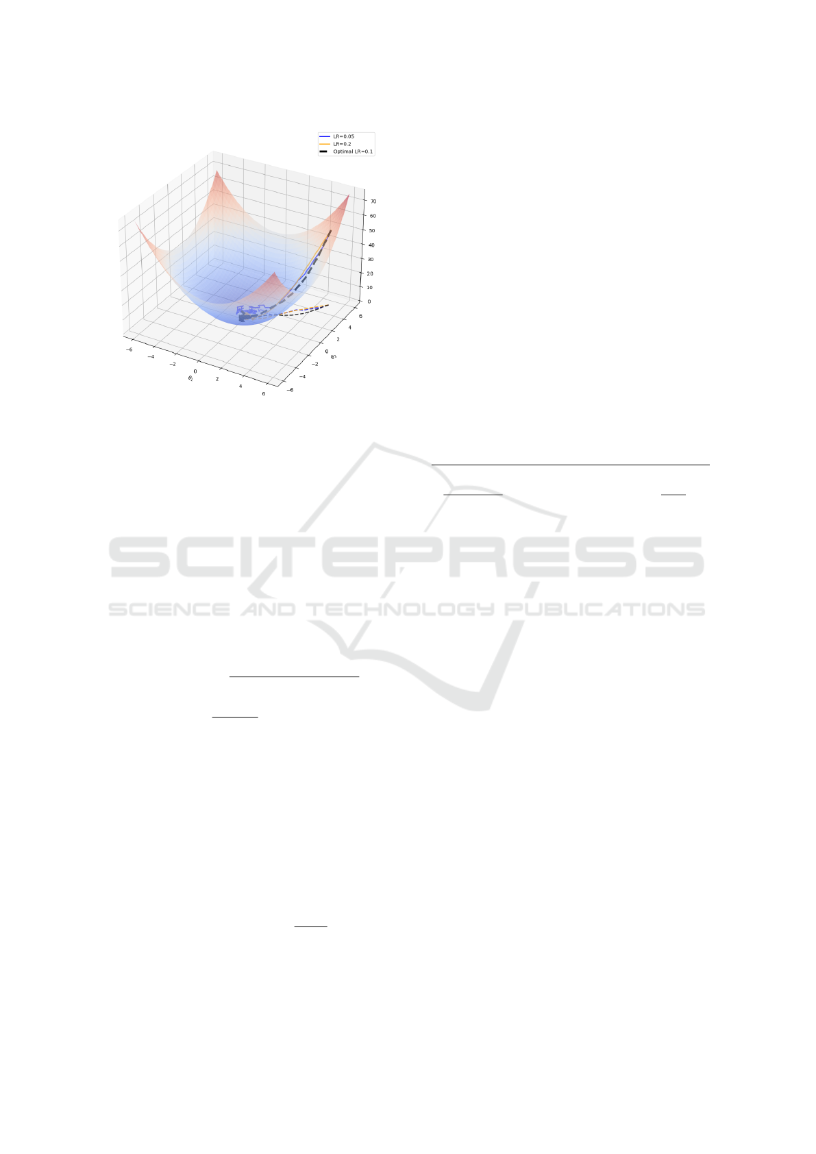
Figure 2: Stochastic gradient descent with different learning

rates. The black solid refers to the optimal learning rate in

stochastic setting.

contrast, FO optimization methods, such as gradient

descent, leverage gradient information to iteratively

update parameters in the direction that minimizes the

objective function. These methods are generally more

efﬁcient than ZO methods, as they can converge to the

optimal solution faster by following the gradient. FO

methods are particularly effective for large-scale op-

timization problems and are widely used in training

deep neural networks.

We deﬁne the ZO gradient estimator, named

Zeroth-Order SGD (ZO-SGD) as in (Malladi et al.,

2023)

∇L(θ) :=

∑

i=1

L(θ + εz

) −L(θ −εz

)

2ε

∇L(θ) ≈

∂L(θ;z)

∂θ

= z

⊤

∇L(θ),

where the random variable z

is a random vector sam-

pled from a normal distribution z

∼ N (0, 1). The in-

ﬁnitesimal constant ε is a small perturbation step size,

also known as the smoothing parameter. After several

tests, we claim that the value of this parameter has lit-

tle impact on the models as long as 10

−3

≤ ε ≤ 10

−5

We selected the value 10

−4

everywhere. The query

budget q is half the number of times the loss is called

to build

∇L.

As ε goes to zero and q = 1, the ZO estimator

approaches the directional derivative of L at θ along

the direction z. Note that since E

∂L(θ;z)

∂θ

= ∇L(θ),

the ZO estimator

∇L is an unbiased estimator of the

FO gradient. This estimation improves as q increases.

One expects to perform a more accurate ZO approxi-

mation towards FO with a higher query budget q. Al-

though ZO methods are back-propagation free, they

suffer from slow convergence. The time needed by

ZO to reach the same accuracy as FO is roughly O(n)

bigger, n being the problem dimension (Nesterov and

Spokoiny, 2017). Most ZO methods have a vari-

ance in the range of O(nq

−1

), q being the number of

queries to the loss (Duchi et al., 2015). This result

also highlights a trade-off between the ZO gradient

estimation and the query complexity. Table 1 sums

up the different convergence rates of three optimiza-

tion classes.

Table 1: For a given optimal solution θ

∗

, the convergence

rate of the relative error varies. i) SO decreases the error

quadratically with the iteration k near the optimum. ii) FO

decreases linearly, with coefﬁcient r ∈ (0, 1): r depends on

the geometry and the conditioning of the objective function.

The closer to zero, the better convergence rate. iii) Eventu-

ally, ZO decreases sub-linearly with coefﬁcient α ∈ (0, 1).

The norm ∥·∥ indicates the Euclidean norm.

Relative Error SO FO ZO

∥θ

k+1

−θ

∗

∥

∥θ

−θ

∗

∥

O(∥θ

−θ

∗

∥) O(r) O



k + 1



We show that the high variance of ZO optimiza-

tion could in fact be in favor of ZO methods in the pre-

training context. As Figure 3 suggests, the variance of

ZO can be a convergence accelerator on a small prob-

lem. On the other hand, using without care can lead

to disastrous results on a larger problem.

3 PRETRAINING

After positive results that show the behaviour of ZO-

SGD is close to FO-SGD in the ﬁne-tuning context,

we explore the more complex pre-training task. Our

goal is to ﬁnd ways to pre-train LMs with ZO, which

means to bring ZO close to FO in terms of ﬁnal loss

value. For this purpose, after understanding that di-

mension and variance are the key, we ﬁrst try to re-

duce the dimension of the problem. Eventually, we

address the ZO-variance issue by implementing two

variance-reduction strategies and study their impact.

3.1 Vanilla Solver

The model trained is Llama2 (Touvron et al., 2023)

with 20M parameters. This small model is built

using the config ﬁle from HuggingFace. In or-

der to remove as many degrees of freedom as

we can, we train with a ﬁxed learning rate, no

weight decay, no momentum or Nesterov acceleration

Zeroth Order Optimization for Pretraining Language Models

117

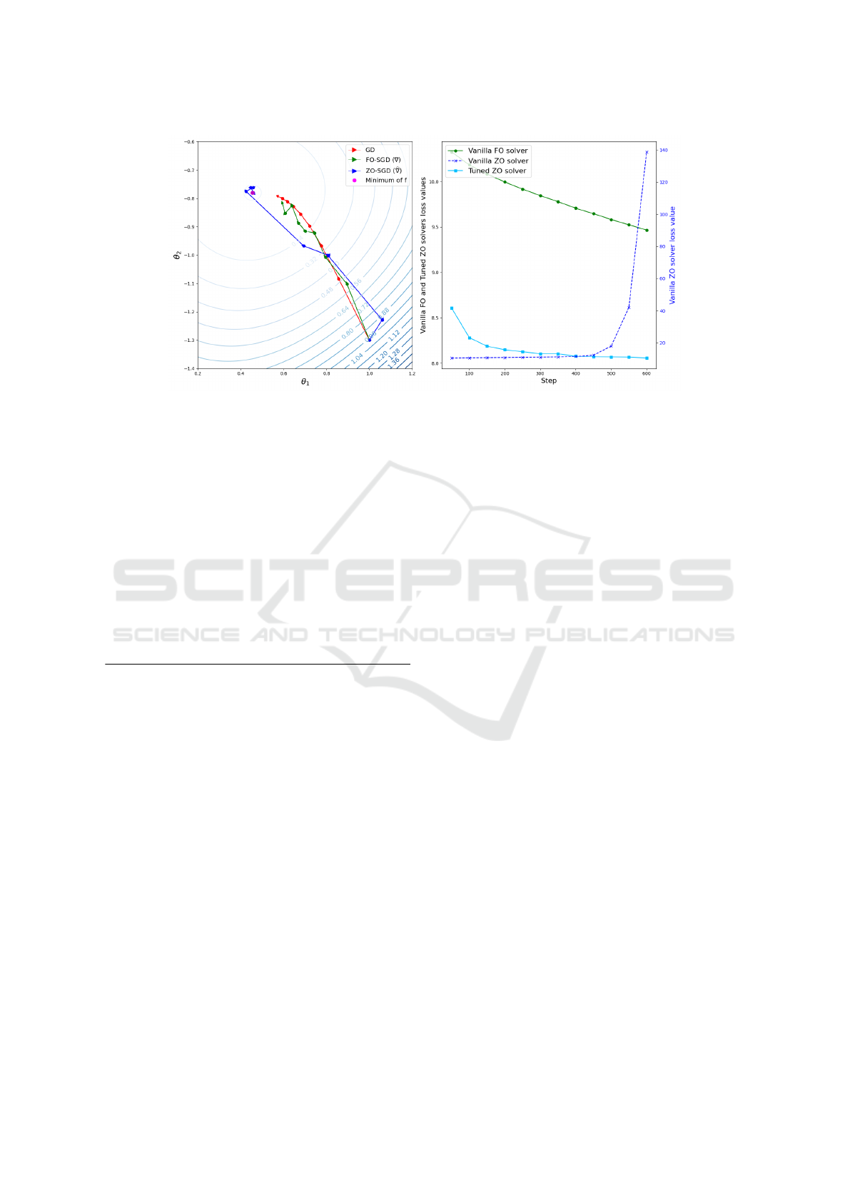
Figure 3: The behaviour of gradient descent (GD) in red, FO stochastic gradient descent (FO-SGD) in green, and its ZO

approximation (ZO-SGD) in blue on a two-dimensional example. The optimal point is denoted by a pink blob (left panel).

An example of pre-training of Llama2 20M with a ZO approximation. A vanilla FO solver in green (without momentum,

learning-rate scheduling, any add-on to improve the solver), a vanilla ZO solver in dark blue which diverges, and a ZO solver

on a smaller dimension with larger query budget q in light blue that eventually converges to the FO optimum loss (right panel).

vanilla FO-SGD vs ZO-SGD. The training dataset is

cosmopedia-100k (Ben Allal et al., 2024) from Hug-

gingFace. We run both experiments on two epochs on

8 V100 GPUs.

Table 2: Comparison of vanilla FO-SGD and ZO-SGD with

two different query budget q for the pre-training task on

Llama2-20M with 8 NVIDIA V100 GPUs.

Method Loss Train Memory Iteration

(cross- time (GB) time

entropy) (h) (s)

FO 8.02 2.5 21.2 0.66

q = 1 diverges 1.5 3.2 0.43

q = 20 8.17 30 3.3 7.14

As expected and shown in Table 2, the high di-

mension of the model leads ZO to behave poorly. For

ZO-SGD to improve the loss, the minimal value is

q = 3. With q = 20, the optimized ZO pre-training

loss gets close to FO but the training time increases

linearly with q while the progress in terms of loss

are logarithmic with q. Though ZO can theoretically

reach FO with very high budget q in the vanilla case,

the high training time and the smaller memory savings

make this solution undesirable. One way to improve

ZO is to reduce the dimension of the problem.

3.2 Reduced Dimension

We try to improve the behaviour of ZO by reduc-

ing the dimension of the problem. Both FO-SGD

and ZO-SGD were run under the same setup as Sec-

tion 3.1. First, we load the FO-trained model from

Section 3.1. Then, we freeze all the parameters of

the model except the ones involved in the last MLP

layer of Llama2-20M. After freezing, there are about

400k parameters remaining (2% of the initial model

size). We reinitialize the unfrozen parameters, then

compare FO-SGD versus ZO-SGD in terms of pre-

training losses. Figure 5 shows a better behaviour

of ZO compared to Section 3.1: with a higher query

budget, ZO can reach FO on a smaller dimension

problem. We suspect this is why ZO is efﬁcient in

ﬁne-tuning. Following this observation, we propose a

strategy for pre-training LMs. At the ﬁrst step update

only a part of the model, say Block 1 with ZO, train

for a few epochs until convergence. At the second

step, re-run the ZO pre-training on another block, say

Block 2, and so on until the whole model is trained.

Details of our method can be found in Section 4.

On Figure 4, FO-variance is roughly 1 000 times

smaller than ZO-variance with q = 1 and 100 times

smaller for q = 20. As expected, one way to reduce

the variance is to increase the budget q but this has a

crucial impact on the training time. Training Llama2-

20M on just 2 epochs with q = 100 takes around 6

days on our setup, versus a couple hours with FO-

SGD, so increasing q is not an option. We won-

der if high-variance really is a ﬂaw for pre-training

LMs with ZO or is there a signiﬁcant impact of this

variance on the optimized pre-training loss. Table 3

shows that a smaller batch size (therefore a higher

variance) has a positive impact on the loss. Following

this observation, we implement a tunable variance-

reduction strategy and observe the same effect there.

ICPRAM 2025 - 14th International Conference on Pattern Recognition Applications and Methods

118

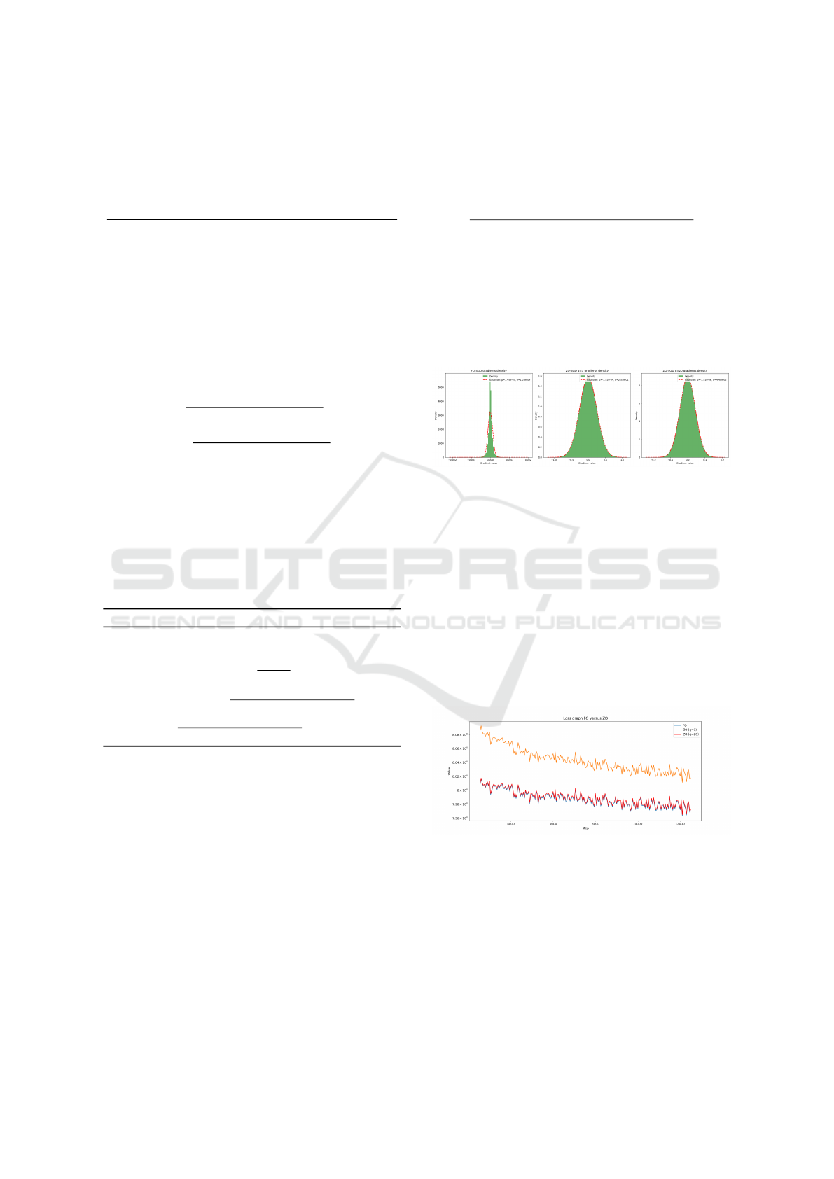
Table 3: ZO-SGD with q = 1 and varying batch size while

pre-training LLama2-20M with reduced dimension.

Batch Loss Train Memory Variance

size (cross- time (GB) ×10

−2

entropy) (h)

2 9.953 1.2 1.6 26.1

4 9.958 1.3 3.1 8.9

8 9.981 1.5 6.1 7.8

3.3 Variance Manipulation

We use the setup of Section 3.2 and consider the spe-

ciﬁc value q = 2. The gradient estimator can then be

expressed as

∇L(θ) = X

+ X

(5)

L(θ + εz

) −L(θ −εz

)

2ε

L(θ + εz

) −L(θ −εz

)

2ε

Since z

and z

are independent, we can build

to be negatively correlated to X

. This strategy

is a common trick in Monte-Carlo simulation (Ross,

2022) and leads the variance of X

+ X

to be smaller

than it should be if z

and z

were sampled indepen-

dently.

For this purpose, at each step of the training, we

build X

the following way:

Algorithm 1: Building X

negatively correlated to X

Require: α ∈ (−1, 1)

1: Sample z

and z

from a normal distribution of

mean 0 and variance 1

2: Deﬁne z

:= αz

√

1 −α

3: Compute X

L(θ + εz

) −L(θ −εz

)

2ε

and

L(θ + εz

) −L(θ −εz

)

2ε

as in (5)

The parameter α tunes the correlation between z

and z

: α = −1 means z

and z

are perfectly neg-

atively correlated, α = 0 means z

and z

are uncor-

related (which is the case by default when sampling

and z

independently), α = 1 means z

and z

are

perfectly positively correlated.

Regarding Table 3, we expect the loss to decrease

as α goes from −1 to zero. Table 4 shows that this is

indeed the case.

4 EXPERIMENTAL DETAILS

Figure 4 gives the gradients density related to

the pre-training of Llama2-20M pre-trained on

Table 4: Comparison of the gradients distribution with vari-

ance manipulation. The optimal loss value is bold.

α Loss Mean Variance

(cross- ×10

−6

×10

−2

entropy)

0.0 7.981 31.3 9.8

-0.5 8.000 -11.1 8.7

-0.9 8.016 9.4 1.5

cosmopedia-100k data, FO versus ZO after one

epoch of 6K steps. The gradients values of FO are

more concentrated than ZO. A higher query budget

q reduces the variance and the mean of ZO, still not

reaching FO.

Figure 4: The gradient density is shown in green. The clos-

est normal distribution is shown in red dashed curve. The

mean and the variance values are mentioned in the legend.

The mean and the variance for FO are lower than ZO. As q

increases, both mean and variance decrease.

Figure 5 shows the pre-training loss trace plot

of Llama2-20M model on cosmopedia-100k text

with different query budget on a reduced dimension

model. For this experiment, only the last MLP layer

of Llama2 is trained, which corresponds to roughly

500K parameters. Figure 5 conﬁrms that ZO is close

to FO with q = 1 (8.02 for ZO and 7.98 for FO). Aug-

menting q allows ZO to reach FO but the training time

increases linearly with q.

Figure 5: The loss curve of FO-SGD is shown in blue.

Curves for ZO-SGD are in orange (q = 1) and red (q = 20).

Increasing the query budget has a positive impact on the

optimized training loss. With high enough budget, ZO can

reach FO.

Figure 6 shows an extension of Figure 5 in pre-

training Llama2-20M layer-by-layer over 600K pa-

rameters. When training a layer, the whole model

but a single layer is frozen and this speciﬁc layer is

reinitialized and retrained. Once this block training

Zeroth Order Optimization for Pretraining Language Models

119

Figure 6: Layer-wise training of Llama2-20M for vanilla

FO (yellow) versus vanilla ZO (blue). Training the full size

model with vanilla FO is shown in purple.

is performed, the trained layer is frozen, and the next

layer is unfrozen and reinitialized. The ﬁrst block is

the embedding layer that includes 10M parameters,

and is trained with vanilla FO in two epochs. The

second block is trained for one epoch with vanilla FO

versus vanilla ZO, and so on. Figure 5 shows that ZO

can reach FO on smaller parameter setting. Moreover,

this result offers ways to improve ZO for pre-training,

for instance adding a momentum that suits ZO.

5 DISCUSSION AND FUTURE

WORK

In this work, we followed several new avenues for

pre-training LMs with ZO, such as variance reduc-

tion and working on a reduced dimension problem.

Low memory cost is a key aspect of ZO training. Its

use could be very relevant in applications such as on-

device training or in situations where memory is lim-

ited. By reducing memory requirements, ZO train-

ing allows larger models to be trained on the same

hardware at the cost of longer training times. Fu-

ture investigations include scaling up blockwise ZO

pre-training to larger models, on small chunks with a

moderate query budget q. The training time will be

longer than for FO, but depending on the goal, the

memory savings may compensate. Ultimately, this

work focused on untuned ZO training. Features such

as adding momentum could improve its efﬁciency and

robustness to scaling.

6 CONCLUSION

This exploratory work unveiled some recently un-

known behaviour of ZO optimization in pre-training

LMs. We established the connection between SO and

FO by studying the optimal learning rate. We also

provided a recepie for a successful application of ZO

in pretraining. First reducing the dimension of the

problem leads to the success of ZO to pre-train LMs

in the sense that vanilla ZO converges to vanilla FO.

Second, the high variance of ZO is not a disadvantage

as it is often thought in the community, but rather is

an asset during the pre-training. As a consequence,

artiﬁcially reducing the variance leads to a higher loss

value. We proposed to pre-train LMs using ZO opti-

mization on a reduced dimension space like blocks of

parameters, because it is the key to a successful pre-

training.

REFERENCES

Amari, S.-i. (1993). Backpropagation and stochastic gra-

dient descent method. Neurocomputing, 5(4-5):185–

196.

Ben Allal, L., Lozhkov, A., Penedo, G., Wolf, T., and von

Werra, L. (2024). Cosmopedia.

Blum, J. R. (1954). Multidimensional stochastic approxi-

mation methods. The annals of mathematical statis-

tics, pages 737–744.

Duchi, J. C., Jordan, M. I., Wainwright, M. J., and

Wibisono, A. (2015). Optimal rates for zero-order

convex optimization: The power of two function eval-

uations. IEEE Transactions on Information Theory,

61(5):2788–2806.

Gautam, T., Park, Y., Zhou, H., Raman, P., and Ha,

W. (2024). Variance-reduced zeroth-order methods

for ﬁne-tuning language models. arXiv preprint

arXiv:2404.08080.

Kaplan, J., McCandlish, S., Henighan, T., Brown, T. B.,

Chess, B., Child, R., Gray, S., Radford, A., Wu, J., and

Amodei, D. (2020). Scaling laws for neural language

models. arXiv preprint arXiv:2001.08361.

Kingma, D. P. (2014). Adam: A method for stochastic op-

timization. arXiv preprint arXiv:1412.6980.

Lehmann, E. and Casella, G. (1998). Theory of Point Es-

timation. Springer Texts in Statistics. Springer New

York.

Liu, S., Kailkhura, B., Chen, P.-Y., Ting, P., Chang, S., and

Amini, L. (2018). Zeroth-order stochastic variance

reduction for nonconvex optimization. Advances in

Neural Information Processing Systems, 31.

Loshchilov, I. and Hutter, F. (2017). Decoupled weight de-

cay regularization. arXiv preprint arXiv:1711.05101.

Malladi, S., Gao, T., Nichani, E., Damian, A., Lee, J. D.,

Chen, D., and Arora, S. (2023). Fine-tuning language

models with just forward passes. Advances in Neural

Information Processing Systems, 36:53038–53075.

Nesterov, Y. and Spokoiny, V. (2017). Random gradient-

free minimization of convex functions. Foundations

of Computational Mathematics, 17(2):527–566.

Prazeres, M. and Oberman, A. M. (2021). Stochastic gra-

dient descent with polyak’s learning rate. Journal of

Scientiﬁc Computing, 89:1–16.

Ross, S. M. (2022). Simulation. academic press.

Shepherd, A. J. (2012). Second-order methods for neu-

ral networks: Fast and reliable training methods for

ICPRAM 2025 - 14th International Conference on Pattern Recognition Applications and Methods

120

multi-layer perceptrons. Springer Science & Business

Media.

Spall, J. C. (1992). Multivariate stochastic approxima-

tion using a simultaneous perturbation gradient ap-

proximation. IEEE transactions on automatic control,

37(3):332–341.

Touvron, H., Lavril, T., Izacard, G., Martinet, X., Lachaux,

M.-A., Lacroix, T., Rozi

ere, B., Goyal, N., Hambro,

E., Azhar, F., et al. (2023). Llama: Open and ef-

ﬁcient foundation language models. arXiv preprint

arXiv:2302.13971.

Vaswani, A., Shazeer, N., Parmar, N., Uszkoreit, J.,

Jones, L., Gomez, A. N., Kaiser, L., and Polo-

sukhin, I. (2017). Attention is all you need. CoRR,

abs/1706.03762.

Wu, X., Ward, R., and Bottou, L. (2018). Wngrad: Learn

the learning rate in gradient descent. arXiv preprint

arXiv:1803.02865.

Zeng, A., Liu, X., Du, Z., Wang, Z., Lai, H., Ding, M.,

Yang, Z., Xu, Y., Zheng, W., Xia, X., Tam, W. L., Ma,

Z., Xue, Y., Zhai, J., Chen, W., Zhang, P., Dong, Y.,

and Tang, J. (2023). Glm-130b: An open bilingual

pre-trained model.

Zhang, Y., Li, P., Hong, J., Li, J., Zhang, Y., Zheng,

W., Chen, P.-Y., Lee, J. D., Yin, W., Hong, M.,

et al. (2024). Revisiting zeroth-order optimization

for memory-efﬁcient llm ﬁne-tuning: A benchmark.

arXiv preprint arXiv:2402.11592.

Zeroth Order Optimization for Pretraining Language Models

121