First Results on Graph Similarity Search in Resting-State Functional

Connectivity Networks Using Spectral and Graph Edit Distances

M. A. G. Carvalho

1,2,3 a

and R. Frayne

2,3,4,5 b

School of Technology, University of Campinas, Brazil

Radiology and Clinical Neurosciences, Hotchkiss Brain Institute, Univ. of Calgary, Canada

Seaman Family MR Research Centre, Foothills Medical Centre, Calgary, Canada

Biomedical Engineering Graduate Program, University of Calgary, Canada

Calgary Image Processing and Analysis Centre, Foothills Medical Centre, Calgary, Canada

Keywords:

Brain Aging, rs-fMRI, Graph Modelling, Bold Signal, Graph Dissimilarity.

Abstract:

The application of graph theory in the modeling and analysis of brain networks has generated both new op-

portunities as well as new challenges in neuroscience. Resting state functional connectivity (RSFC) networks

studied with graphs is an important ﬁeld of investigation because of the potential beneﬁts in understanding

function in healthy individuals and identifying evidence of brain diseases and injury in patients. This work

is unique because it applies information retrieval techniques to create ranked lists from RSFC graph theory-

derived networks. In our analysis, we used a sample of whole-brain resting-state functional magnetic reso-

nance imaging (rs-fMRI) data obtained from Young (n = 10, age: 20.1 ± 2.1) and Old (n = 10, 65.6 ± 0.4)

sex-balanced groups drawn from a healthy, i.e., neurotypical, cohort. We estimated two well-known distance

metrics (graph edit distance and graph spectral distance) and by using information-retrieval graph ranking

methods achieved precision measures at the top-5 positions of ranked lists of up to 80%.

1 INTRODUCTION

Functional magnetic resonance imaging (fMRI) has

been used to understand human brain functions in

both healthy subjects and patients for over three

decades (Lv et al., 2018). Since the 2000s, resting-

state fMRI (rs-fMRI) data, acquired in the absence

of a task, has lead to the development of functional

connectivity (FC) measures. Resting state approaches

due to the relative simplicity of acquisition and con-

ceptual simplicity of analysis are frequently applied

to study healthy individuals and across patients with

a variety of neurological and psychiatric conditions.

Conditions like Alzheimer’s disease and Tourette’s

syndrome, for example, are associated with abnormal

alterations in connectivity between different brain re-

gions (Dai et al., 2019; Yang et al., 2023).

Among the many existing strategies to analyze rs-

fMRI data, graph theoretical approaches have been

applied due to their ability to investigate large, com-

plex networks. We denote a graph G = (V, E) by using

https://orcid.org/0000-0002-1941-6036

https://orcid.org/0000-0003-0358-1210

V to represent a set of nodes or vertices and E ⊆ V

to describe the set of connecting edges. Typically, the

analysis of RSFC networks is done by obtaining and

comparing measurements obtained from the graph G,

such as modularity, clustering coefﬁcient, between-

ness centrality, global efﬁciency, and network degree

and density(Bullmore and Sporns, 2009). Graphs

have been used in modeling resting-state functional

connectivity (RSFC) networks by several research

groups (Wu et al., 2023; Wright et al., 2021; Hry-

bouski et al., 2021).

Graph similarity search methods, used com-

monly in information science, represents alternate ap-

proaches to analyze RSFC networks. They have not

been previously applied to study RSFC networks in

either healthy individuals or patients. Graph simi-

larity search seeks to retrieve relevant graphs from

a user-speciﬁed graph-structured query (Liang and

Zhao, 2017). Usually, distance or similarity metrics

are used to compute overall measures that account

for the underlying relationships amongst the graphs.

Ranked lists from the perspective of a graph query

can be calculated using these distance or similarity

Carvalho, M. A. G. and Frayne, R.

First Results on Graph Similarity Search in Resting-State Functional Connectivity Networks Using Spectral and Graph Edit Distances.

DOI: 10.5220/0013261400003911

Paper published under CC license (CC BY-NC-ND 4.0)

In Proceedings of the 18th International Joint Conference on Biomedical Engineering Systems and Technologies (BIOSTEC 2025) - Volume 1, pages 357-362

ISBN: 978-989-758-731-3; ISSN: 2184-4305

357

measures.

We used two metrics to calculate distance in

graphs: 1) graph edit distance (GED), and 2) graph

spectral distance (GSD). GED estimates the dissimi-

larity measure between two graphs, G

and G

, that is

calculated by ﬁnding the minimum number of stan-

dard graph edit operations needed to transform G

into G

(Riesen, 2015). The standard set of edit

operations includes insertions and deletions of both

nodes and edges. GSD provides a second measure

of similarity between G

and G

. Typically, GSD

uses the eigenvectors and eigenvalues of the graph

adjacency or Laplacian matrix and computes the Eu-

clidean distance between the two graphs (Wilson and

Zhu, 2008). To our knowledge, graph similarity

search methods have not been applied to RSFC net-

works in healthy individuals or patients.

In this paper, we used graph similarity search ap-

proaches to assess RSFC whole-brain networks of

Young and Old healthy (neurotypical) individuals.

Ranked lists, based on GED and GSD, were used to

evaluate our graphs.

We examined the following research question:

Can GED or GSD be used as an efﬁcient measure

of dissimilarity of RSFC networks of individuals in

different age groups? Section 2 presents our analysis

pipeline and describes the key methodological steps,

including how we modeled RSFC networks and the

calculated GED and GSD. Section 3 presents the ex-

perimental results and Section 4 summarizes our con-

clusions, study limitations and future work.

2 COMPUTING GRAPH

DISTANCES AND RANKED

LISTS

In this section, we describe the approach used to com-

pute network distances from a graph model represent-

ing RSFC networks. Our approach consists of three

main steps (outlined by the dotted squares in Figure

1). Each step is described in the following three Sub-

sections.

2.1 Dataset and FC Matrix

Data from the Calgary Normative Study (CNS) (Mc-

Creary et al., 2020) was used in this work. The CNS is

an ongoing study, begun in 2013, that focuses on col-

lecting quantitative MR data from healthy adults over

18 years. All MR data were acquired from individuals

residing in or near the Calgary, Alberta, Canada who

provided informed written consent. Data acquisition

was approved by the University of Calgary Conjoint

Health Research Ethics Board. The CNS acquires

several types of quantitative MR neuroimaging data

including rs-fMRI. We selected N = 20 individuals

from the CNS database. The demographics for the

Young and Old groups are shown in Table 1. Both

groups had a 50% : 50% female : male sex balance.

Table 1: Sex (Female, Male) and group (Young and Old)

demographics. Unpaired t-tests were used to determine sig-

niﬁcance by sex and by group.

Sex Count Age(years) p-value

Female n = 10 44.3 ± 23.7 0.948

Male n = 10 43.6 ± 23.8

Cohort Count Age(years)

Young n = 10 20.1 ± 2.1 < 0.001

Old n = 10 65.6 ± 0.4

Total n = 20 44.0 ± 23.8

In the CNS study, rs-fMRI data were acquired

by measuring spatially localized ﬂuctuations in the

blood oxygen level dependent (BOLD) signal. This

signal included noise and artifact from a variety of

sources. A processing pipeline that comprised sev-

eral steps was applied to extract the BOLD ﬂuctu-

ations from this signal. The pipeline included the

analysis and preparation of rs-fMRI images, as de-

scribed in (Sidhu, 2023). Brieﬂy the pipeline in-

cluded: skull striping using the Brain Extraction

Tool (BET), motion correction using the Motion

Correction FMRIB Linear Image Registration Tool

(MCFLIRT), interleaved slice-time correction, spatial

smoothing, temporal high-pass ﬁltering, independent

component analysis (ICA) and functional-structural

registration. Structural and functional image prepro-

cessing was carried using publicily available soft-

wares FreeSurfer(Fischl, 2012) and FSL(Smith et al.,

2004), respectively. For each individual, a FC matrix

of size 200 × 200 was calculated. This matrix size

corresponded to segmenting the whole-brain into 200

anatomical regions using the Schaefer-Yeo cortical at-

las. After analyzing the quality of the rs-fMRI data, it

was decided to exclude graph nodes from the left and

right limbic networks because of signal loss result-

ing from MR susceptibility artifacts. Finally, Fisher’s

r–to–z transformation was applied to the Pearson cor-

relation values. An example FC matrix is shown in

Figure 2(a), where the colors are associated with the

Pearson correlation coefﬁcient values.

BIOIMAGING 2025 - 12th International Conference on Bioimaging

358

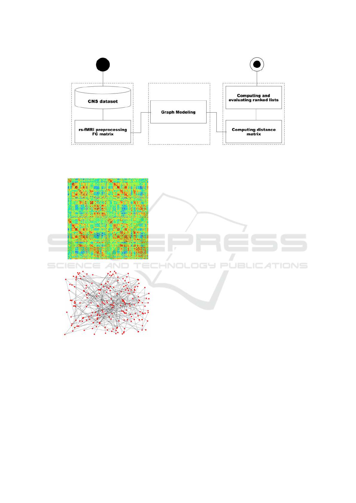
Figure 1: Analysis pipeline overview showing main steps (denoted by dotted boxes, from left to right): 1) creation of the

functional connectivity (FC) matrix, 2) modeling of the graph and 3) estimation and ranking of graph distance). CNS =

Calgary Normative Study(McCreary et al., 2020).

(a)

(b)

Figure 2: (a) Example of Pearson FC correlation matrix

and (b) its corresponding graph of one individual from the

CNS dataset. For visualization purposes, the graph in (b)

was built for a graph density equal to 5%.

2.2 Graph Model for RSFC Network

An undirected graph is an ordered pair G = (V, E)

with a node (or vertex) set V and an edge (or link)

set E connecting the nodes (Chung, 2019). An undi-

rected graph yields a symmetric connectivity matrix.

Each anatomical region resulting from the brain par-

cellation is a graph node u ∈ V and pairs of nodes

represent a connection. Each element of the FC ma-

trix represents the edge e ∈ E between a pair of nodes.

The associated r-to-z transformed Pearson correlation

value of the RSFC network is the edge weight. In

order to characterize a RSFC network as a “small-

world” network (where most nodes maintain only a

few direct connections) several strategies are com-

monly employed including assuming the entire net-

work is a graph, applying a thresholding operation,

creating a spanning tree and adopting a speciﬁc graph

density (Deery et al., 2023; Jockwitz and Caspers,

2021).

We chose to use the graph density modeling ap-

proach with an initial seed given by maximum span-

ning tree (MaxST). The reason for this choice is that

using MaxST ensures that we obtain a connected

graph, which is necessary for calculating the GSD.

Furthermore, MaxST iteratively selects the most rel-

evant edges in its construction. In this work, the

MaxST is derived from an undirected graph for each

participant, built with N nodes that matched the size

of FC matrix, and a number of edges E selected to

represent a pre-speciﬁed fraction of the graph den-

sity, i.e., a number of selected entries (or links) in the

FC matrix. We used only positive Pearson correlation

values (z ⩾ 0) and set the main diagonal of the FC

matrix to zero to exclude self-connections.

Based on literature ﬁndings, we considered using

graph densities ranging from [1%, 25%] (Marek et al.,

2015) to [22%, 40%](Grady et al., 2016). To better

ﬁne tune the graph density range, we considered two

criteria: First, we used the modularity metric (M) as a

reference metric because 94% of studies demonstrate

decrease in M with age(Deery et al., 2023). Modu-

larity measures the topological organization of whole

brain FC networks in a set of groups, where it is possi-

First Results on Graph Similarity Search in Resting-State Functional Connectivity Networks Using Spectral and Graph Edit Distances

359

ble to distinguished dense internal (intra-module) and

sparse external (inter-module) connectivity. Second,

values of M ⩾ 0.3 are generally associated with non-

random module structure and, thus, are thought to re-

ﬂect brain topological organization. After this anal-

ysis we decided to use a graph density ranging from

[1%, 10%].

Figure 2(b) shows an example graph, correspond-

ing to a percentage of edges of a complete graph con-

structed from the FC correlation matrix of Figure 2(a).

2.3 Graph Distance

Two distance measurements were considered:

1) Graph Edit Distance (GED) is a dissimilarity mea-

sure from the number as well as the strength of the op-

erations that have to be applied to transform a source

graph (G

) into a target graph (G

)(Riesen, 2015).

GED is deﬁned by:

GED(G

, G

) = min

∑

c(e

) (1)

where c(e

) denotes the cost of the i

edit opera-

tion. In this work, considering that graphs (RSFC net-

works) have the same dimension and the same label-

ing of nodes anatomical regions), edit operations are

limited to the deletion and insertion of edges, with the

cost of each operation being equal to 1. In addition, a

variant of GED that considers only the weights of the

added or removed edges was also calculated.

2) Graph Spectral Distance (GSD) is obtained from

the spectrum of the graph derived from its adjacency

matrix representation using eigenvalue decomposi-

tion. The graph spectrum is the set of ordered eigen-

values s

= {λ

, λ

, ..., λ

|V|

}, where i refers to the

graph label, | V | represents the size or the number

of nodes of the matrix G corresponding to the RSFC

network. GSD is deﬁned by:

GSD(G

, G

) =

∑

− s

)

(λ

− λ

)

+ ... +(λ

|V|

− λ

|V|

)

(2)

where the subscript denotes the number of the eigen-

value and the superscript, refers to the graphs 1 and

2. In this work, the GSD is computed by using the

Laplacian matrix L = D − A, where D is the diago-

nal degree matrix and A corresponds to the graph ad-

jacency matrix. Additionally, GSD was also calcu-

lated from the Euclidean distance between the second

smallest eigenvector of each RSFC matrix, known as

the Fiedler vector (Wilson and Zhu, 2008).

2.4 Ranked Lists and Evaluation

We adapted the notation deﬁned by (Pedronette et al.,

2016). Let C = {G

, G

, ..., G

} be a collection of

graphs, where n =| C | is the size of C. Based on

the distance measure, d(·, ·), a ranked list τ

can be

computed as a permutation of the collection C in re-

sponse to a query graph G

. If G

is ranked before G

in the ranked list of G

then d(G

, G

) ≤ d(G

, G

Every graph G

∈ C can produce a ranked list. There-

fore, a set of ranked lists R = {τ

, τ

, ..., τ

} can

be obtained. In order to evaluate the list of ranked

lists, we compute the precision p (the fraction of rele-

vant list entries among the retrieved list) at position k

(i.e., p@k). In other words, p@k is the fraction of the

number of relevant items in the ﬁrst k positions of the

ranked list.

3 RESULTS AND DISCUSSIONS

Figure 3 plots the p@5 to p@10 values as a function

of graph density for GED and GSD computed accord-

ing to a graph query for identifying the Young group.

The most relevant information (around 80% of preci-

sion) were obtained at the top-5 positions of ranked

lists, i.e., at p@5. They are compatible with what

the information retrieval literature suggests regarding

the value of k << n where n =| C | is the number of

graphs(Pedronette et al., 2016). An 80% value for

p@5 means that for the obtained ranked lists, four of

the ﬁrst ﬁve items were relevant and correctly identi-

ﬁed a RSFC network from an individual in the Young

group.

In this type of study it is also possible to observe

how representative a given RSFC network is for either

the Young or Old groups. The p@5 sequence across

the ten ranked lists for GED was (80%, 80%, 80%,

80%, 60%, 100%, 100%, 80%, 80%, 60%), where

each element corresponds to one of the ten individuals

in the Young group. These values were obtained for a

graph density of 1%. Some networks reached 100%

precision while others only achieved 60%. Lower pre-

cision values may serve as indicators or biomarkers

that should result in further investigations for a spe-

ciﬁc individual. Finally, the analysis of ranked lists

with higher precision values can contribute to deﬁn-

ing graph density values or range of values that are

most appropriate to represent a RSFC network.

BIOIMAGING 2025 - 12th International Conference on Bioimaging

360

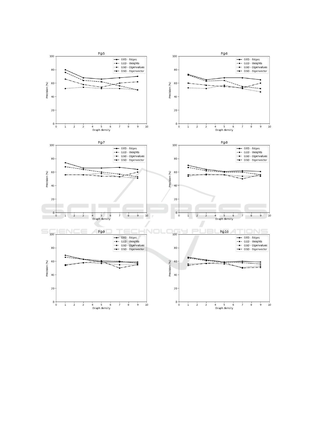
Figure 3: Average precision p@k (k = 5 to 10) to rank individuals in the Young group.

4 CONCLUSIONS

In the current study we have shown that techniques

used in the area of graph similarity search can be ap-

plied to analyze RSFC networks. The use of ranked

lists is useful in the information retrieval processes,

such as identifying Young or Older individuals as in

this work. As well, ranked lists may being applied for

other types of tasks, such as the clustering of RSFC

networks of individuals with different types of dis-

eases. The best precision values obtained in this work

were around 80% and suggests that there is a possibil-

ity of increase through the use of re-ranking and rank-

ing aggregation techniques (Pedronette et al., 2016).

First Results on Graph Similarity Search in Resting-State Functional Connectivity Networks Using Spectral and Graph Edit Distances

361

We intend to expand this study by analyzing the entire

set of images collected by the CNS, considering the

inclusion and exclusion criteria indicated in (Sidhu,

2023), and observing the quality of the scans in each

of the functional networks in the preprocessing stage.

Further studies should extend these whole-brain re-

sults and individually examine sensory and associa-

tive functional networks that are consistently reported

in the literature: Visual, Sensorimotor, Dorsal Atten-

tion, Ventral Attention, Limbic, Frontoparietal, and

Default Mode.

ACKNOWLEDGEMENTS

This study was ﬁnanced in part by the Coordination of

Improvement of Higher Education Personnel - Brazil

(CAPES) - Finance Code 001. Marco Carvalho wish

to express their gratitude to the S

ao Paulo Research

Foundation/Fundac¸

ao de Amparo

a Pesquisa do Es-

tado de S

ao Paulo (FAPESP grant 2023/02302-6). We

also acknowledge the assistance of Kau

e TN Duarte,

Abhi S Sidhu, and Cherly R McCreary, from Univer-

sity of Calgary.

REFERENCES

Bullmore, E. and Sporns, O. (2009). Complex brain net-

works: graph theoretical analysis of structural and

functional systems. Nature Reviews Neuroscience,

10:186–198.

Chung, M. K. (2019). Brain Network Analysis. Cambridge

University Press, United Kingdom.

Dai, Z., Lin, Q., Li, T., Wang, X., Yuan, H., Yu, X., He, Y.,

and Wang, H. (2019). Disrupted structural and func-

tional brain networks in Alzheimer’s disease. Neuro-

biology of Aging, 75:71–82.

Deery, H. A., Paolo, R. D., Moran, C., Egan, G. F., and

Jamadar, S. D. (2023). The older adult brain is less

modular, more integrated, and less efﬁcient at rest:

A systematic review of large-scale resting-state func-

tional brain networks in aging. Psychophysiology,

60:e14159.

Fischl, B. (2012). Freesurfer. Neuroimage, 62(2):774.

Grady, C., Sarraf, S., Saverino, C., and Campbell, K.

(2016). Age differences in the functional interac-

tions among the default, frontoparietal control, and

dorsal attention networks. Neurobiology of Aging,

41:159–172.

Hrybouski, S., Cribben, I., McGonigle, J., Olsen, F., Carter,

R., Seres, P., Madan, C. R., and Malykhin, N. V.

(2021). Investigating the effects of healthy cogni-

tive aging on brain functional connectivity using 4.7

T resting-state functional magnetic resonance imag-

ing. Brain Structure and Function, 226:1067–1098.

Jockwitz, C. and Caspers, S. (2021). Resting-state network

in the course of aging - differential insights from stud-

ies across the lifespan vs. amongst the old. European

Journal of Physiology, 473:793–803.

Liang, Y. and Zhao, P. (2017). Similarity search in graph

databases: A multi-layered indexing approach. In

2017 IEEE 33rd International Conference on Data

Engineering (ICDE), pages 783–794.

Lv, X. H., Wang, X. Z., Tong, X. E., Williams, X. L., Za-

harchuk, X. G., Zeineh, X. M., Goldstein-Piekarski,

X. A., Ball, X. T., Liao, X. C., and Wintermark, X. M.

(2018). Resting-state functional MRI: Everything that

nonexperts have always wanted to know. AJNR Am J

Neuroradiol, 39:1390–1399.

Marek, S., Hwang, K., Foran, W., Hallquist, M. N., and

Luna, B. (2015). The contribution of network organi-

zation and integration to the development of cognitive

control. PLoS Biology, 13(12):e1002328.

McCreary, C. R., Salluzzi, M., Andersen, L. B., Gobbi,

D., Lauzon, L., Saad, F., Smith, E. E., and Frayne,

R. (2020). Calgary normative study: Design of a

prospective longitudinal study to characterise poten-

tial quantitative MR biomarkers of neurodegeneration

over the adult lifespan. BMJ Open, 10:e038120.

Pedronette, D. C. G., Almeida, J., and Torres, R. S. (2016).

A graph-based ranked-list model for unsupervised dis-

tance learning on shape retrieval. Pattern Recognition

Letters, 83:357–367.

Riesen, K. (2015). Structural Pattern Recognition with

Graph Edit Distance. Springer, Switzerland.

Sidhu, A. S. (2023). Decreasing Brain Functional Network

Segregation with Healthy Aging. MSc thesis, Biomed-

ical Engineering, University of Calgary, Calgary, AB,

Canada.

Smith, S. M., Jenkinson, M., Woolrich, M. W., Beckmann,

C. F., Behrens, T. E. J., Johansen-Berg, H., Bannis-

ter, P. R., Luca, M. D., Drobnjak, I., Flitney, D. E.,

Niazy, R. K., Saunders, J., Vickers, J., Zhang, Y., Ste-

fano, N. D., Brady, J. M., and Matthews, P. M. (2004).

Advances in functional and structural mr image anal-

ysis and implementation as fsl. Neuroimage, 23:Suppl

1:S208–19.

Wilson, R. C. and Zhu, P. (2008). A study of graph spectra

for comparing graphs and trees. Pattern Recognition,

41(12):2833–2841.

Wright, L. M., Marco, M. D., and Venneri, A. (2021). A

graph theory approach to clarifying aging and disease

related changes in cognitive networks. Frontiers in

Aging Neuroscience, 13:676618.

Wu, K., Jelfs, B., Mahmoud, S. S., Neville, K., and Fang,

J. Q. (2023). Tracking functional network connectiv-

ity dynamics in the elderly. Frontiers in Neuroscience,

17:1146264.

Yang, Y., Yang, H., Yu, C., Ni, F., Yu, T., and Luo, R.

(2023). Alterations in the topological organization of

the default-mode network in Tourette syndrome. BMC

Neurology, 23:390.

BIOIMAGING 2025 - 12th International Conference on Bioimaging

362