Anomaly Detection Methods for Maritime Search and Rescue
Ryan Sime
1
and Rohan Loveland
2
1
Dept. of Electrical Eng. and Computer Science, South Dakota School of Mines and Technology, Rapid City, SD, U.S.A.
2
New College of Florida, Sarasota, FL, U.S.A.
Keywords:
Anomaly Detection, Maritime Search and Rescue, SeaDronesSee, Variational Autoencoders, Isolation
Forests, Farpoint.
Abstract:
Anomaly detection methods are employed to find swimmers and boats in open water in drone imagery from the
SeaDronesSee dataset. The anomaly detection methods include variational autoencoder-based reconstruction
loss, isolation forests, and the Farpoint algorithm. These methods are used with both the original feature space
of the data and the encoded latent space representation produced by the variational autoencoder. We selected
six images from the dataset and break them into small tiles, which are ranked by anomalousness by the various
methods. Performance is evaluated based on how many tiles must be queried until the first positive tile is found
compared to a random selection method. We find that the reduction of tiles that must be queried can range
into factors in the thousands.
1 INTRODUCTION
Anomaly detection is a rapidly expanding field with
a wide variety of methods and applications that has
seen a surge of research performed in the last few
years (Nassif et al., 2021). Applications range from
monitoring system health (Lee et al., 2015) to de-
tecting manufacturing defects (Nakazawa and Kulka-
rni, 2019) to identifying abnormal activity to protect
cyber-physical critical infrastructure (Vegesna, 2024).
In this work, we apply anomaly detection to mar-
itime search and rescue by examining drone imagery
containing swimmers and boats in open water. The
SeaDronesSee dataset is a collection of frames taken
from footage captured by drones hovering over Lake
Constance (Kiefer et al., 2023) (Varga et al., 2022).
It contains a variety of imagery along multiple spec-
tra and resolutions with a wide array of camera an-
gles and altitudes. We selected six images in which
the drone is at a sufficiently high altitude to pro-
vide a large viewing area and where the camera an-
gle is perpendicular to the water in order to provide
a bird’s-eye view. On these images, three methods
of anomaly detection are applied: variational autoen-
coder (VAE) reconstruction loss, isolation forests, and
the Farpoint algorithm. Each method allows us to
determine an object’s anomalousness in an image by
providing rankings of anomalousness. If objects of
interest are anomalous, we are able to reduce the
amount of time that a human would spend manually
monitoring footage or even extend the algorithm to
automate the process in real time.
2 RELATED WORK
Anomaly detection methods are typically categorized
by their feature maps and models. Shallow methods
tend to have larger feature spaces that do not extract
important features while deep methods learn to ab-
stract the most important features but at the cost of
increased computational complexity. These methods
typically fall into four types of models: classification,
probabilistic, reconstruction, and distance (Ruff et al.,
2021).
Previous maritime search and rescue research with
drone imagery approaches the problem as an object
detection problem using deep convolutional neural
networks (Kiefer et al., 2023) (Kiefer and Zell, 2023)
or as a standard probabilistic path search problem
(Schuldt and Kurucar, 2016) instead of an anomaly
detection problem.
One approach to anomaly detection on images is
using reconstruction error from autoencoders (Zhou
and Paffenroth, 2017). Autoencoders learn to recon-
struct the dominant class well and become sensitive
to anomalies. Variational autoencoders (VAEs) ex-
tend this by constraining the encoded representation
764
Sime, R. and Loveland, R.
Anomaly Detection Methods for Maritime Search and Rescue.
DOI: 10.5220/0013263000003905
Paper published under CC license (CC BY-NC-ND 4.0)
In Proceedings of the 14th International Conference on Pattern Recognition Applications and Methods (ICPRAM 2025), pages 764-770
ISBN: 978-989-758-730-6; ISSN: 2184-4313
Proceedings Copyright © 2025 by SCITEPRESS – Science and Technology Publications, Lda.

to a multi-variate normal distribution (Kingma and
Welling, 2013). These can be further extended to con-
volutional autoencoders (Chen et al., 2017) or Gaus-
sian Mixture Model autoencoders (Zong et al., 2018).
Viewing maritime search and rescue as an
anomaly detection problem offers a few approaches.
Distance-based techniques can be used to isolate
points that differ from the ”normal” points. Isolation
forests give an anomaly score to points based on the
average path length of the binary search trees created
when partitioning points in order to isolate them (Liu
et al., 2008). Probabilistic techniques, such as ker-
nel density estimation, operate under the assumption
that data points that are considered anomalous should
have a low probability density where a threshold can
be applied to low probability points to extract anoma-
lies (Rosenblatt, 1956).
3 DATA
3.1 Pre-Processing
The SeaDronesSee dataset, acquired in 2021, is a col-
lection of over 54,000 frames taken from footage cap-
tured by drones hovering over Lake Constance. It
contains a variety of imagery along multiple spectra
and resolutions with camera angles ranging from 0
◦
to 90
◦
and altitudes ranging from 5 to 260 meters. We
narrow down the frames to only include frames where
the viewing angle is between 85
◦
to 90
◦
and the drone
altitude is above 100 meters. Of these frames, we se-
lected 6 frames from roughly the same area contain-
ing multiple objects that were taken at an altitude of
approximately 255 meters.
The frames are broken up into square tiles with
side lengths of 16 pixels and with 3 channels for RGB.
A new tile is created every 8 pixels both vertically and
horizontally in order to create overlapping tiles. This
results in 104,880 tiles which are flattened to create
vectors with 768 features. The tile size was chosen
based on the ratio of object pixels to water pixels. Dif-
ferent tile sizes were explored and tiles that were sig-
nificantly larger or smaller than the object had poor
performance. Under the assumption that the resolu-
tion of the image and the size of the object of interest
are known, the choice of tile size becomes primar-
ily based on altitude as objects will occupy a varying
amount of pixels in a frame based on the field of view.
The dataset has annotated metadata which in-
cludes labels and bounding box coordinates for each
object, the latter of which can be used to identify tiles
containing objects. Each pixel inside the bounding
box is evaluated to determine if the tiles are positive
tiles. If a tile is identified as a positive, it is given a
class label and a unique object ID.
3.2 Object Isolation
To determine each method’s effectiveness in real-
world scenarios in which there is likely only one ob-
ject in the water, we isolate each object individually
by temporarily removing positive object tiles from the
dataset so that only a single object’s positive tiles and
water tiles remain. This allows us to determine an
object’s individual anomalousness without being af-
fected by previously identified objects.
3.3 Dimensionality Reduction
The curse of dimensionality is an infamous obstacle
in machine learning that can easily lead to increased
computational complexity or overfitting. To mitigate
this problem, we reduce the dimensionality of the fea-
ture space by using the VAE’s learned encoding abil-
ity to produce 16-dimensional latent space represen-
tations of the original feature space and compare per-
formance to the original feature space.
4 METHODS
4.1 Random Baseline
A random baseline algorithm can be used to calculate
the expected values of the numbers of tiles that would
have to be queried in order to find a positive tile that
contains an object.
To find the random selection expected values: let
N be the total number of tiles, P = {positive tile p
i
:
p
i
contains an object}, P = |P |, B be the number of
empty water tiles, and X
i
be the number of positive
tiles found.
Let X
1
− 1 be the number of tiles queried before a
tile p
i
∈ P is found. Then
E[X
1
] =
B
P + 1
+ 1 =
N + 1
P + 1
. (1)
and
E[X
2
] = E[X
1
] +
N
′
+ 1
P
′
+ 1
(2)
where
N
′
= N −
N + 1
P + 1
and P
′
= P − 1 (3)
such that, with some algebra, we can calculate that
the expected value of the number of queries to find
the nth positive tile of an object is
E[X
n
] = nE[X
1
] (4)
Anomaly Detection Methods for Maritime Search and Rescue
765

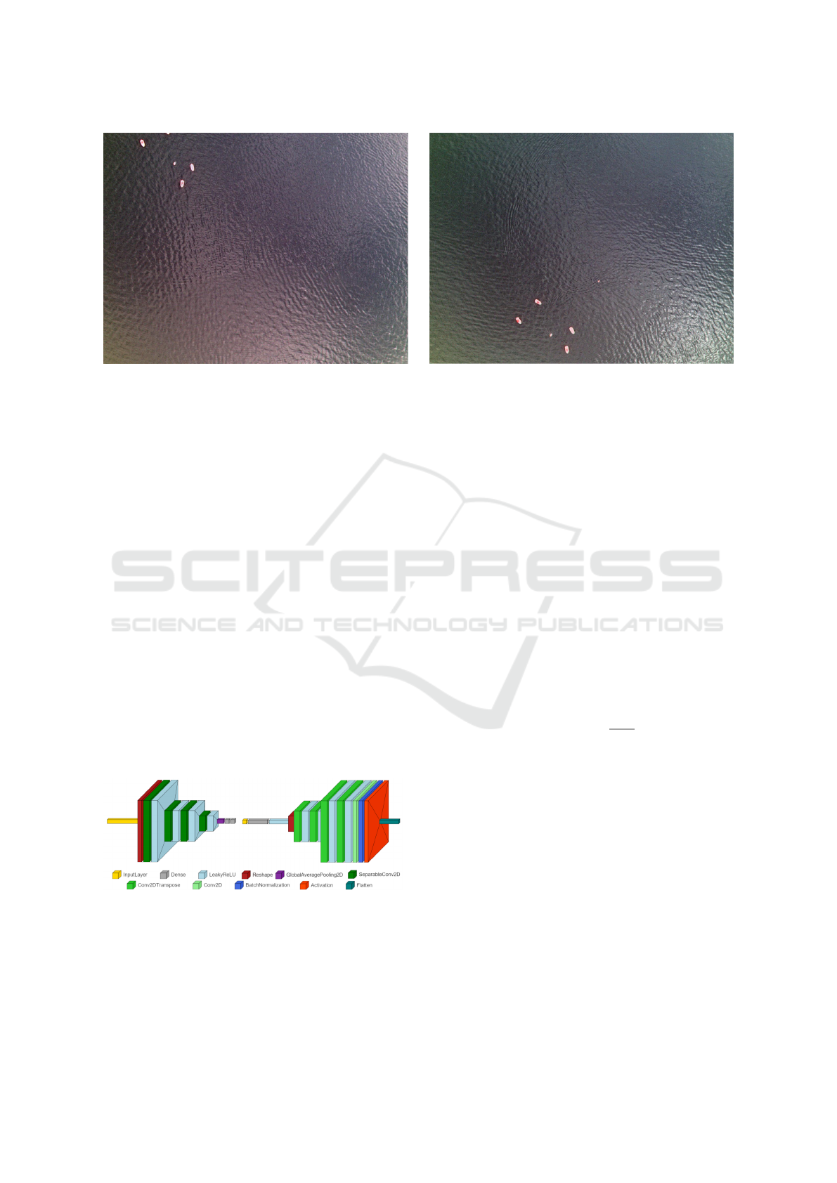
Figure 1: Two of the six selected images.
4.2 Variational Auto Encoders
Deep autoencoders (AE) can be used as a method for
anomaly detection based on the idea that they learn to
encode ”normal” samples such that anomalous sam-
ples will be poorly reconstructed (Zhou and Paffen-
roth, 2017). This is achieved by reducing the feature
space to a low-dimensional latent space in between
the encoder and decoder. An anomalousness score for
each input can be calculated using the autoencoder by
calculating the mean squared error of the reconstruc-
tion loss of the reconstructed image and the input im-
age.
An extension of the autoencoder, the VAE was
proposed to improve performance, where the prob-
ability density of the latent space is shaped to be a
multi-variate normal density.
The two primary differences in implementation
between AE’s and VAE’s are the addition of a ran-
domly sampled noise term in the latent space and a
modified loss function. These are described briefly
below, along with the specific model architecture
shown in Fig. 2.
Figure 2: The variational autoencoder model architecture.
4.2.1 Encoder Network
The inputs for the encoder are the flattened tile vec-
tors which are reshaped into a 16x16x3 tensor. The
encoder has four two-dimensional separable convo-
lution layers that perform a depthwise convolution
(Kaiser et al., 2017) separately on each channel fol-
lowed by a pointwise convolution (Keras, b) mixing
the channels: the first using a 5x5 kernel and a stride
of 1, the second using a 3x3 kernel and a stride of
2, the third using a 5x5 kernel and a stride of 1, and
the fourth using a 3x3 kernel with a stride of 2. Each
layer is followed by a LeakyReLU activation layer.
The resulting 4x4x64 tensor goes through a two-
dimensional global average pooling layer (Keras, a),
and into two parallel 16-node dense layers to produce
the encoded outputs that correspond to the means and
variances of the VAE’s multi-variate normal distribu-
tion.
4.2.2 Sampler
The sampler adds random normal noise ε scaled by λ
= 0.05 to the mean. The resulting latent space z is:
z = µ + λεe
logσ
2
2
(5)
which is based off of the implementation of (Chollet,
2021).
4.2.3 Decoder Network
The decoder feeds the sampled latent space into a
4096-node dense layer and reshapes it into an 8x8x64
tensor. There are four two-dimensional convolutional
transpose layers that mirror the encoder layers with
the same kernels and strides as their encoder counter-
parts. Each convolutional transpose is followed by a
LeakyReLU activation layer. A final convolution with
3 filters, a 1x1 kernel, and a stride of 1 is applied to
reduce the filter space to three channels. Batch nor-
malization and a sigmoid activation are applied be-
fore flattening the output to the original vector of size
3072.
ICPRAM 2025 - 14th International Conference on Pattern Recognition Applications and Methods
766

4.2.4 Training
The model was trained with the Adamax optimizer us-
ing a batch size of 64 over 50 epochs. The total train-
ing loss for each epoch is the average of each batch’s
loss, which is the sum of the average binary cross-
entropy reconstruction loss and the Kullback-Leibler
divergence loss:
loss = loss
r
+ loss
KL
(6)
where
loss
r
=
1
S
S
∑
i=0
M−1
∑
j=0
BCE(x,r) (7)
and
loss
KL
= −
1
2S
L
∑
i=0
(1 + log σ
2
− µ
2
i
− e
logσ
2
) (8)
where BCE is the binary cross-entropy function, x and
r are the original and reconstructed images, S is the
batch size, M is the number of features in the tiles,
and µ
i
and σ
i
are the mean and standard deviation in
the latent space of dimensionality L such that {µ
i
,σ
i
:
i ∈ 1..L}.
4.2.5 Reconstruction Error Based
Anomalousness
An anomalousness score based on the mean squared
reconstruction error, α
RE
, is implemented with:
α
RE
=
1
M
M
∑
i=1
(I
rec
(i) − I
input
(i))
2
(9)
where I
rec
and I
input
are the flattened arrays of the re-
constructed and input images at index i and M is the
total number of pixels.
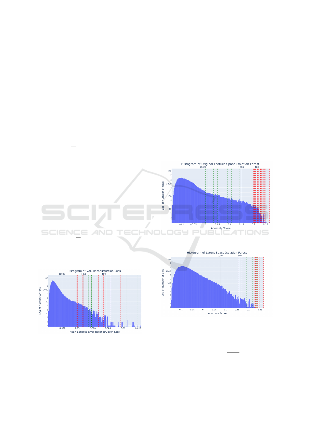
Figure 3: α
RE
for each tile encoded into the latent space of
dimensionality L=16.
A histogram of α
RE
, with the top 100 anomalies,
is shown in Fig. 3. Green lines indicate the first de-
tected tile of objects that are swimmers and red lines
indicate the first detected tile of objects that are boats.
A bimodal distribution would support a division be-
tween a ’normal’ population and anomalous classes.
Upon inspection, we can observe that there are several
distinct groupings of tiles.
4.3 Isolation Forests
Isolation Forests are a tree-based anomaly detection
technique based on randomly selecting node divisions
in order to isolate a point in feature space (Liu et al.,
2008). Finding the average path length for each point
over a large number of trees allows for an estimate
of the probability density, which can then be used to
calculate an anomalousness score.
We used sci-kit learn’s implementation of isola-
tion forests on the original 768-dimensional feature
space data as well as the 16-dimensional latent space
representation from the VAE encoder.
Figure 4: α
IF
scores for each tile from the original 768-
dimension feature space.
Figure 5: α
IF
scores for each tile from the encoded latent
space representation.
The corresponding anomalousness scores, which
we designate as α
IF
for consistency, are based on:
α
IF
= −(0.5 − 2
−E(h(z))
c(N)
) (10)
where c(N) is the average search length for a dataset
of size N,
c(N) = 2 ln N − 1 + γ − 2(N − 1)/N (11)
Anomaly Detection Methods for Maritime Search and Rescue
767

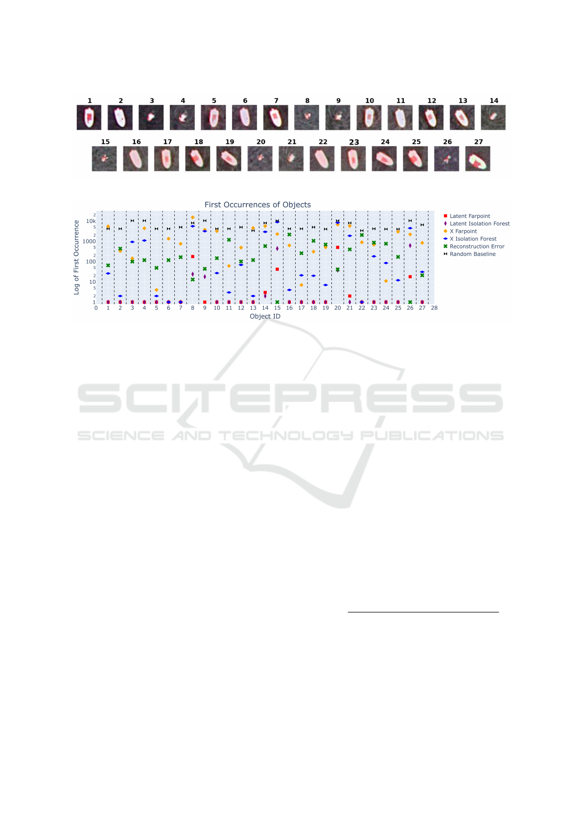
Figure 6: 40x40 pixel tiles of each object and their corresponding IDs.
Figure 7: Number of queries before first occurrence per object for each method.
where γ is Euler’s constant. We negate 10 in order to
make more positive values indicate increasing anoma-
lousness.
The histograms of α
IF
for isolation forests for the
original feature space as well as the latent space are
shown in Fig. 4 and Fig. 5 respectively. Green lines
indicate the first detected tile of objects that are swim-
mers and red lines indicate the first detected tile of ob-
jects that are boats. Distinct notches can be noted here
as well, with the latent space anomaly score groupings
being more pronounced.
4.4 Farpoint Algorithm
The Farpoint algorithm is based on treating anomaly
detection as a rare class detection problem, rather
than binary classification or anomalousness scoring
(Loveland and Amdahl, 2019) (Loveland and Kaplan,
2022). Farpoint is typically used in a active semi-
supervised mode, where samples are presented to the
user who supplies a label for the sample. The algo-
rithm uses the label to attempt to find a sample from
a different class each time, in the process minimiz-
ing the overall number of queries required to find all
classes. In this mode, Farpoint works both as an algo-
rithm for rare class detection as well as a classifier for
imbalanced datasets.
Farpoint can also run in an unsupervised mode,
circumventing the oracle/user entirely, by providing
positive tiles with the same label and every other tile
with a different label. We used Farpoint in this mode
because the tiles contained a variety of objects that
were all deemed to be of interest. In this mode it
is clear that no classifier will result, but the order in
which the tiles are presented can be seen as a ranking
for anomalousness.
5 RESULTS
In the 6 images that were selected, there are 27 objects
in total: 18 boats and 9 swimmers. These objects and
their respective IDs are shown in Fig. 6. In Fig. 7,
we show the number of queries that were required to
find the first occurrence of an object using the various
methods, where X is the original feature space. The
efficiency of each method can be determined by com-
paring the number of queries until first occurrence
to the expected number of queries from the random
baseline. First occurrence efficiency is used instead
of standard classification methods as only one posi-
tive tile needs to be found in order for positive identi-
fication as an object of interest. First occurrence effi-
ciency (FOE) is defined as follows:
FOE =
query # of first pos. tile using random selection
query # of first pos. tile using algorithm
(12)
Table 1 provides the FOEs for each object and
each method. These results show that Farpoint (FP)
and isolation forests (IF) operating on the latent space
representation dramatically outperformed the same
experiments on the original feature space X , the re-
construction error for most objects, and the random
baseline. The experiments on the latent space resulted
ICPRAM 2025 - 14th International Conference on Pattern Recognition Applications and Methods
768

Table 1: First Occurrence Efficiencies (FOE) for each method on each object.
1 2 3 4 5 6 7 8 9 10 11 12 13 14
# of Positive Tiles 24 24 9 9 24 24 20 12 9 24 24 20 30 12
Random Baseline 4175 4175 10437 10437 4175 4175 4970 8028 10437 4175 4175 4970 3367 8028
Latent FP 4175.00 4175.00 10 437.00 10 437.00 4175.00 4175.00 4970.00 45.36 10 437.00 4175.00 4175.00 4970.00 3367.00 2676.00
Latent IF 4175.00 4175.00 10 437.00 10 437.00 4175.00 4175.00 4970.00 334.50 579.83 4175.00 4175.00 4970.00 3367.00 4014.00
X FP 0.76 12.61 72.48 2.38 1043.75 3.10 6.57 0.53 2.78 1.31 68.44 10.16 0.74 1.43
X IF 160.58 2087.50 11.16 9.51 2087.50 4175.00 4970.00 1.45 3.31 154.63 1391.67 72.03 1683.50 2.73
Rec Error 64.23 9.58 104.37 88.45 85.20 35.38 30.12 617.54 237.20 28.40 3.50 49.21 28.29 13.77
15 16 17 18 19 20 21 22 23 24 25 26 27
# of Positive Tiles 9 24 24 20 25 9 12 30 24 25 25 9 15
Random Baseline 10437 4175 4175 4970 4014 10437 8028 3367 4175 4014 4014 10437 6523
Latent FP 248.50 4175.00 4175.00 4970.00 4014.00 20.79 4014.00 3367.00 4175.00 4014.00 4014.00 579.83 6523.00
Latent IF 23.77 4175.00 4175.00 4970.00 4014.00 274.66 8028.00 3367.00 4175.00 4014.00 4014.00 16.89 6523.00
X FP 4.57 6.65 596.43 16.14 7.90 1.56 1.40 3.76 6.13 364.91 1.35 4.75 7.75
X IF 1.17 1043.75 198.81 248.50 573.43 1.26 4.28 3367.00 22.94 47.22 334.50 2.34 210.42
Rec Error 10437.00 1.93 16.18 4.70 5.77 254.56 20.07 1.64 4.86 5.26 23.61 10 437.00 310.62
in a positive tile being found on the first query for ev-
ery boat and several swimmers, as well as requiring
significantly less queries for the swimmers that were
not immediately queried compared to the experiments
on the original feature space.
It is worth noting that reconstruction error outper-
formed the latent space experiments on the objects
that were not queried immediately by the latter. It
can be speculated that these objects that have more
defined features, which were difficult for the VAE to
reconstruct, ended up clustered tightly in the encoded
feature space meaning that both Farpoint and isolation
forests needed more splits for these objects compared
to the other objects, but still significantly fewer than
their original feature space counterparts.
6 CONCLUSION
Anomaly detection methods are shown to signifi-
cantly reduce the amount of time that is spent inspect-
ing images for objects of interest. In particular, using
a variational autoencoder that is sensitive to anoma-
lous samples to encode the feature space into a latent
space shows a dramatic improvement.
The efficiency of Farpoint on the latent space is
limited not only to first occurrence efficiency but also
computation time. Not only is the high computational
complexity of Farpoint dampened by reducing the di-
mensionality, but querying positive tiles faster means
that fewer overall queries are necessary.
With some algorithmic alterations and reduction
in computation time, future work can be extended
from a static dataset to real-time streaming data.
A corresponding machine learning-based augmenta-
tion of maritime search and rescue with deployable
drones with anomaly detection capabilities could sig-
nificantly aid in reducing manpower requirements and
improving search success.
REFERENCES
Chen, M., Shi, X., Zhang, Y., Wu, D., and Guizani, M.
(2017). Deep feature learning for medical image anal-
ysis with convolutional autoencoder neural network.
IEEE Transactions on Big Data, 7(4):750–758.
Chollet, F. (2021). Deep learning with Python. Simon and
Schuster.
Kaiser, L., Gomez, A. N., and Chollet, F. (2017). Depthwise
separable convolutions for neural machine translation.
arXiv preprint arXiv:1706.03059.
Keras. Globalaveragepooling2d layer. https://keras.io/api/
layers/pooling layers/global average pooling2d/.
Keras. Separableconv2d layer. https://keras.io/api/layers/
convolution layers/separable convolution2d/.
Kiefer, B., Kristan, M., Per
ˇ
s, J.,
ˇ
Zust, L., Poiesi, F., An-
drade, F., Bernardino, A., Dawkins, M., Raitoharju,
J., Quan, Y., et al. (2023). 1st workshop on maritime
computer vision (macvi) 2023: Challenge results. In
Proceedings of the IEEE/CVF Winter Conference on
Applications of Computer Vision, pages 265–302.
Kiefer, B. and Zell, A. (2023). Fast region of inter-
est proposals on maritime uavs. In 2023 IEEE In-
ternational Conference on Robotics and Automation
(ICRA), pages 3317–3324. IEEE.
Kingma, D. P. and Welling, M. (2013). Auto-encoding vari-
ational bayes. arXiv preprint arXiv:1312.6114.
Lee, E. K., Viswanathan, H., and Pompili, D. (2015).
Model-based thermal anomaly detection in cloud dat-
acenters using thermal imaging. IEEE Transactions
on Cloud Computing, 6(2):330–343.
Liu, F. T., Ting, K. M., and Zhou, Z.-H. (2008). Isolation
forest. In 2008 eighth ieee international conference
on data mining, pages 413–422. IEEE.
Loveland, R. and Amdahl, J. (2019). Far point algorithm:
active semi-supervised clustering for rare category de-
tection. In Proceedings of the 3rd International Con-
ference on Vision, Image and Signal Processing, pages
1–5.
Loveland, R. and Kaplan, N. (2022). Combining active
semi-supervised learning and rare category detection.
In Advances in Deep Learning, Artificial Intelligence
and Robotics, pages 217–229. Springer.
Anomaly Detection Methods for Maritime Search and Rescue
769

Nakazawa, T. and Kulkarni, D. V. (2019). Anomaly de-
tection and segmentation for wafer defect patterns us-
ing deep convolutional encoder–decoder neural net-
work architectures in semiconductor manufacturing.
IEEE Transactions on Semiconductor Manufacturing,
32(2):250–256.
Nassif, A. B., Talib, M. A., Nasir, Q., and Dakalbab, F. M.
(2021). Machine learning for anomaly detection: A
systematic review. Ieee Access, 9:78658–78700.
Rosenblatt, M. (1956). Remarks on some nonparametric
estimates of a density function. The annals of mathe-
matical statistics, pages 832–837.
Ruff, L., Kauffmann, J. R., Vandermeulen, R. A., Mon-
tavon, G., Samek, W., Kloft, M., Dietterich, T. G., and
M
¨
uller, K.-R. (2021). A unifying review of deep and
shallow anomaly detection. Proceedings of the IEEE,
109(5):756–795.
Schuldt, D. W. and Kurucar, J. (2016). Maritime search and
rescue via multiple coordinated uas.
Varga, L. A., Kiefer, B., Messmer, M., and Zell, A.
(2022). Seadronessee: A maritime benchmark for de-
tecting humans in open water. In Proceedings of the
IEEE/CVF winter conference on applications of com-
puter vision, pages 2260–2270.
Vegesna, V. V. (2024). Machine learning approaches for
anomaly detection in cyber-physical systems: A case
study in critical infrastructure protection. Interna-
tional Journal of Machine Learning and Artificial In-
telligence, 5(5):1–13.
Zhou, C. and Paffenroth, R. C. (2017). Anomaly detec-
tion with robust deep autoencoders. In Proceedings
of the 23rd ACM SIGKDD international conference
on knowledge discovery and data mining, pages 665–
674.
Zong, B., Song, Q., Min, M. R., Cheng, W., Lumezanu,
C., Cho, D., and Chen, H. (2018). Deep autoencoding
gaussian mixture model for unsupervised anomaly de-
tection. In International conference on learning rep-
resentations.
ICPRAM 2025 - 14th International Conference on Pattern Recognition Applications and Methods
770