Belief Re-Use in Partially Observable Monte Carlo Tree Search

Ebert Theeuwes

1 a

, Gabriele Venturato

1 b

and Gavin Rens

2 c

KU Leuven, Dept. of Computer Science, B-3000 Leuven, Belgium

Computer Science Division, Stellenbosch University, Stellenbosch, South Africa

Keywords:

Partially Observable Markov Decision Processes, Monte Carlo Tree Search, Locality-Sensitive Hashing,

Transposition Nodes, Belief Re-Use.

Abstract:

Partially observable Markov decision processes (POMDPs) require agents to make decisions with incomplete

information, facing challenges like an exponential growth in belief states and action-observation histories.

Monte Carlo tree search (MCTS) is commonly used for this, but it redundantly evaluates identical states

reached through different action sequences. We propose Belief Re-use in Online Partially Observable Plan-

ning (BROPOP), a technique that transforms the MCTS tree into a graph by merging nodes with similar

beliefs. Using a POMDP-speciﬁc locality-sensitive hashing method, BROPOP efﬁciently identiﬁes and reuses

belief nodes while preserving information integrity through update-descent backpropagation. Experiments on

standard benchmarks show that BROPOP enhances reward performance with controlled computational cost.

1 INTRODUCTION

Partially observable Markov decision processes

(POMDPs) (Smallwood and Sondik, 1973) are noto-

riously used to model problems where an agent needs

to make sequential decisions (planning) in a partially

observable stochastic environment. In these prob-

lems, the agent only has a ‘belief’ about the cur-

rent state that is represented by a belief state, that

is, a probability distribution over all possible ex-

plicit states. POMDPs are hard problems (Papadim-

itriou and Tsitsiklis, 1987; Mundhenk et al., 2000).

Their belief state space grows exponentially on the

number of state variables (curse of dimensionality),

and also the number of action-observation histories

suffers from an exponential growth (curse of his-

tory) (Kaelbling et al., 1998). Monte Carlo tree

search (MCTS) is a standard technique to tackle these

‘curses’, both in planning (Silver and Veness, 2010;

Browne et al., 2012) and in reinforcement learn-

ing (Schrittwieser et al., 2020). However, when dif-

ferent action-observation sequences lead to the same

state, they are still treated as separate nodes in the

MCTS tree, meaning they are expanded and evalu-

ated multiple times. This is further complicated by

the fact that POMDPs work on an uncountable set of

https://orcid.org/0009-0009-2220-5166

https://orcid.org/0000-0002-0048-0898

https://orcid.org/0000-0003-2950-9962

belief states, where a slight variation in the belief dis-

tribution can correspond to the same explicit state.

Therefore, we propose a new technique for Be-

lief Re-use in Online Partially Observable Planning

(BROPOP), where we move from an MCTS tree to

a graph, by merging nodes that correspond to simi-

lar beliefs. Speciﬁcally, we leverage locality-sensitive

hashing (LSH) (Datar et al., 2004) by introducing our

novel POMDP-specialized hashing algorithm to ef-

ﬁciently compare a new node with all the existing

ones already in the MCTS graph. Moreover, we ad-

dress the problem of backpropagating the values in

this graph in an update-descent fashion (Czech et al.,

2021), which ensures limited information leakage.

Finally, we evaluate our method on a set of stan-

dard POMDP benchmarks, showing that belief re-use

positively impacts reward performance while keeping

the computational performance under control.

2 BACKGROUND

2.1 Partially Observable Markov

Decision Processes

POMDPs model the same underlying problem as

Markov decision processes (MDPs), but they add par-

tially observable states observed via noisy sensors.

634

Theeuwes, E., Venturato, G. and Rens, G.

Belief Re-Use in Partially Observable Monte Car lo Tree Search.

DOI: 10.5220/0013265200003890

Paper published under CC license (CC BY-NC-ND 4.0)

In Proceedings of the 17th International Conference on Agents and Artiﬁcial Intelligence (ICAART 2025) - Volume 2, pages 634-645

ISBN: 978-989-758-737-5; ISSN: 2184-433X

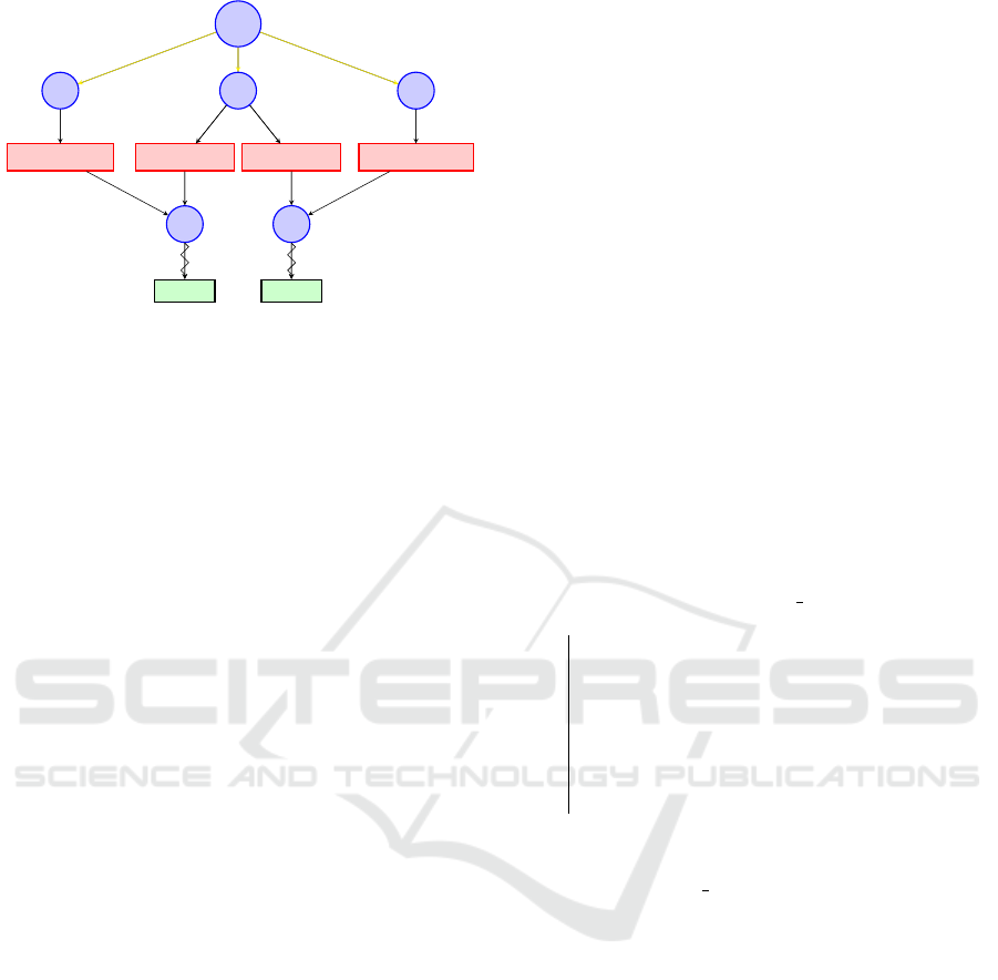
Figure 1: Our proposed method, BROPOP. When a new observation node O

is added to the Monte Carlo search tree, we use

locality-sensitive hashing (LSH) to efﬁciently compare the belief state ( ) of O

with the ones that are hashed into the same

‘bucket’ (O

). A similarity distance measure, ∆, is used to decide whether to merge two nodes if they are within a given ε

threshold.

POMDPs (Smallwood and Sondik, 1973) are repre-

sented by the tuple (S, A, T, R, Z, O), where, S is the

set of states, A is the set of actions and Z is the set of

observations. The transition function T : S ×A ×S →

[0, 1] speciﬁes the probability T (s, a, s

′

) of ending up

in state s

′

after executing an action a in state s. The

reward function R: S ×A → R speciﬁes the reward

R(s, a) of executing action a in state s. The observa-

tion function O: S×A×Z →[0, 1] speciﬁes the proba-

bility O(s

′

, a, z) of observing z when executing action

a and ending up in state s

′

As an example, imagine a robot in a grid world

that is equipped with a noisy sensor. The robot does

not know in which state it is, but after taking an ac-

tion, it will get an observation from the environment

(via its noisy sensor), which will tell the robot some-

thing about its actual state via its observation func-

tion. The job of a planner algorithm is to ﬁnd the

optimal policy, that is, the best action in each state.

This is done by taking into account the uncertainty of

the current state. A belief state is a probability dis-

tribution over all possible states, represented as a list

of state-probability pairs (s, b(s)) for each state s ∈ S.

Each pair (s, b(s)) indicates the probability b(s) that

the agent is in state s. By making use of the transi-

tion and observation function, we are able to keep the

belief state up to date throughout the problem. The

update of the belief state is done as follows (Somani

et al., 2013):

′

) = ηO(s

′

, a

t−1

, z

)

∑

s∈S

T (s, a

t−1

, s

′

t−1

(s),

where b

(s) denotes the probability (belief) of being

in the state s at time t, and η is a normalization con-

stant. The full belief state b

= τ(b

t−1

, a

t−1

, z

) at time

t is the calculation of b

′

) for each state s

′

2.2 Partially Observable Monte Carlo

Planning

Monte Carlo tree search (MCTS) is a tree search algo-

rithm that was designed to be an efﬁcient alternative

to full scale tree search while still converging to the

optimal policy at inﬁnity (Browne et al., 2012). The

MCTS algorithm operates by generating the search

tree in a step-by-step manner. Each iteration con-

sists out of four steps (Levine, 2017; Browne et al.,

2012): (i) Tree traversal/Selection, (ii) Node expan-

sion, (iii) Rollout/Simulation, (iv) Backpropagation.

For POMDPs, such an MCTS tree contains obser-

vation nodes (with a belief state) and action nodes.

Observation nodes represent the current observation.

These nodes are followed by action nodes, represent-

ing each possible action (see Figure 1).

Partially Observable Monte-Carlo Planning

(POMCP) is an algorithm introduced by Silver and

Veness (2010), that uses MCTS for online planning

in POMDPs. The selection step (i) is to branch down

the tree until reaching a leaf node. This tree traversal

is done by repeatedly choosing the next action node

from the current observation node by the use of the

UCB1 (Safﬁdine et al., 2012) function:

UCB1(x) = µ(x) + c ·

ln(p(x))

n(x)

where µ(x) is the average reward attached to the ac-

tion node x. Each action node starts with µ set to

zero and is updated in the backpropagation step. c

is the exploration constant that balances the trade-

off between exploration and exploitation. The visi-

tation count of a node x, denoted by n(x), represents

the number of times the node was visited in the al-

gorithm. It also gets updated in the backpropagation

step. p(x) is the total number of payoffs, that is, the

number of times the node was considered to be tra-

versed. Because each action node has only one parent

Belief Re-Use in Partially Observable Monte Carlo Tree Search

635

observation node, this value is just the visitation count

of the parent observation node. When the desired

action node is chosen, we make use of a generator

function to generate a possible next observation. This

observation is sampled according to the correct prob-

abilities in order to ﬁnd the next observation node,

which also generates an immediate reward that gets

accumulated for later. Upon reaching a leaf node, a

node expansion (ii) is done, which creates a new ob-

servation node action nodes pair. If the desired depth

has not yet been reached, a random simulation (iii)

is performed. Finally, the accumulated rewards are

propagated back (iv) in the tree to update the average

rewards and visitation counts. These accumulated re-

wards are also discounted such that steps farther in the

future have smaller weight.

2.3 Similarity Distance Measures

In order to re-use observation nodes, a measure of

similarity between belief states is essential. This re-

quires distance measures that quantify the difference

between two probability distribution vectors (belief

states). In this work, we consider the following dis-

tance measures.

2.3.1 Euclidean Distance

The Euclidean distance (Cohen et al., 1997) measures

the length of a straight line connecting two points in a

Euclidean space:

d(p, q) =

∑

i=1

−q

)

2.3.2 Hellinger Distance

The Hellinger distance (Chen et al., 2019) is an f-

divergence. This means it was speciﬁcally designed to

measure the difference between two probability distri-

bution vectors. It is deﬁned by the following formula:

H(p, q) =

√

∑

i=1

(

√

−

√

)

We can rewrite it by using the Euclidean distance:

H(p, q) =

√

q). (1)

2.3.3 Jensen–Shannon Divergence

The Jensen–Shannon divergence (Chen et al., 2019)

is a symmetric variant of the Kullback–Leibler diver-

gence (Kullback, 1951). It is also an f-divergence and

has the following formula:

JSD(p ∥ q) =

(p ∥m) +

(q ∥ m),

where, m is:

m =

p + q

and D

is the Kullback–Leibler divergence:

(p ∥q) =

∑

i=1

log





We do not use Kullback–Leibler divergence by itself

because it is asymmetric, meaning that it produces

different results based on argument order. While this

can be useful in likelihood theory with distinct prior

and posterior distributions (Shlens, 2014), our ap-

proach merges observation nodes without such dis-

tinction, making a symmetric measure more suitable.

2.4 Information Leak Problem

There is an intrinsic problem to backpropagating in an

MCTS graph, that is, where certain nodes have mul-

tiple parent nodes, compared to an MCTS tree. This

is known as the information leak problem (Safﬁdine

et al., 2012), visualized in Figure 2. For the sake of

simplicity, the discount factor here is set equal to 1

and there are no immediate rewards. Imagine being in

observation node O

, one can either go to action node

or A

. Here, the action node A

is always selected,

because of the higher average reward (µ) and a lower

visitation count (n). By bad luck, action node A

got

an average reward of 0.4 over a limited amount of 6

visitations. However, action node A

actually leads

to a higher expected reward. The intrinsic problem is

that sufﬁcient information is actually in the tree, but it

is just not accessible from action node A

, because it

was backpropagated to action node A

instead. Exam-

ining A

, we see that it has the highest average reward

in the observable tree. All its rewards were also back-

propagated through observation node O

. If we com-

pute the average rewards of O

’s child action nodes,

weighted by their visitation counts, we ﬁnd that ac-

tion node A

actually is superior. Thus, although this

information is present in the tree, it is not accessible

from A

(because the rewards were backpropagated to

instead), creating the information leak problem.

3 RELATED WORK

Similar node re-use techniques have already been re-

searched for games. In this setting, a node that gets

re-used is called a transposition node. This occurs for

ICAART 2025 - 17th International Conference on Agents and Artiﬁcial Intelligence

636

Root

(µ:0.5, n:17)

(µ:0.5, n:5)

E = 0.5

(µ:0.4, n:6)

E = 0.6

(µ:0.66, n:21)

Figure 2: Information leak problem. The yellow lines repre-

sent underlying paths from the root to the observation node.

The zigzag lines point to the expected reward of going down

that path.

example in the game of chess, where a speciﬁc board

state can be reached via a variety of different move

combinations. Instead of doing search separately for

all nodes representing this board state, it is better to

merge them together in one transposition node. Nev-

ertheless, there are still notable differences between

MCTS trees for games and POMDPs. First, games

have a different tree structure (no observation and ac-

tion nodes but separate nodes for each player). Sec-

ond, a discount factor is not used when backpropagat-

ing in games. That is because one is only concerned

with winning the game (and thus backpropagating a

win, loss or draw), and not with maximizing some

long term reward.

Safﬁdine et al. (2012) introduce a framework for

transposition nodes in MCTS trees for games, that

deals with the information leak problem. They solve it

by introducing a new measure for representing the av-

erage reward at a certain edge. It is called the adapted

score and makes use of a hyperparameter for the

depth. This adapted score is calculated every time one

needs the average reward for the UCB1 function. It is

calculated by using the average rewards for all edges

deeper in the tree, until the desired depth is reached.

This method can deal with the information leak, but

it will create a big overhead to recalculate this score

over and over again. Choe and Kim (2019) intro-

duce a new backpropagation scheme. What they do is

standard update-descent backpropagation (backprop-

agating according to the path one descends from) but

upon reaching a transposition node, they do update-

all (backpropagating to all accessible nodes) until a

certain height is reached. This will ensure that the

average rewards suffer less from information leak.

However, it suffers from the bad side effects associ-

ated with update-all, such as overhead, as described

by Safﬁdine et al. (2012). Finally, Czech et al. (2021)

measure the information leak in a node above a trans-

position node during tree traversal. This can be done

by comparing their average rewards with each other.

When the difference between them is larger than some

threshold, we know that there is a leak of information.

When this is measured, the search is stopped and a

correction value is backpropagated instead.

4 BROPOP

The main idea of belief re-use is that if two beliefs are

similar enough, then they should be merged into the

same node. Speciﬁcally, given that a belief is a proba-

bility distribution represented as a vector, the smaller

the distance between two vectors, the more similar

they are. This means that when the distance between

two belief states is smaller than a certain threshold,

their observation nodes should be merged together.

This happens in the Merge procedure, accessed in Al-

gorithm 1.

Data: o

node

, a

node

, z

Result: New observation node o

node2

Initialization: o

node2

← get child(a

node

, z);

if o

node2

is nothing then

b ← τ(o

node

.b, a

node

.a, z);

create o

node2

;

node2

.b ← b;

node2

.n ← 0;

node2

.z ← z;

push(a

node

.c, o

node2

);

Merge(o

node2

);

end

return o

node2

;

Algorithm 1: The Get o

node

procedure, to create, and pos-

sibly merge, a new observation node, given the current ob-

servation o

node

and action a

node

nodes, as well as the obser-

vation from the environment z. For a given node, .b is the

belief, .a is the action, .c is the list of children and .n is the

visitation count.

In the Merge procedure, the observation node is

hashed to its bucket and then compared with all nodes

in there. If its distance with one node is smaller than

a certain threshold, they should be merged together.

The factorization of the belief state space into buckets

is performed via LSH.

Our method consists of two main novelties. First,

we use locality-sensitive hashing (LSH) to efﬁciently

compare a new observation node to already existing

nodes in the MCTS graph. Second, we use a back-

propagation technique with minimum overhead to up-

date the information in the nodes. Their synergy in

an MCTS-like algorithm resulting in Belief Re-use in

Online Partially Observable Planning (BROPOP).

Belief Re-Use in Partially Observable Monte Carlo Tree Search

637

4.1 Locality-Sensitive Hashing

A major time drawback of merging observation nodes

is the overhead from comparing nodes. That is be-

cause we need to compare each new observation

node with each existing observation node. By us-

ing locality-sensitive hashing (LSH), this overhead

is heavily reduced. LSH is a hashing technique that

takes in as input a vector (i.e. a belief) and returns a

bucket, represented by an integer. LSH tries to maxi-

mize the probability of a hash collision occurring be-

tween similar vectors. A hash collision happens when

distinct vectors get assigned the exact same bucket.

This way, a speciﬁc bucket will only contain vectors

that are similar or close to one another.

According to the deﬁnition of LSH, the collision

probability of two vectors x and y is proportional to

the similarity between them (Charikar, 2002):

Pr [h(x) = h(y)] ∝ sim(x, y).

These collision probability functions can further be

manipulated by using multiple instances of the same

hash function. This means that two vectors only col-

lide when they have the same bucket for every used

hash function. For example, when one would use N

of such hash functions, the collision probability will

take the following value:

Pr [h

(x) = h

(y)] = Pr [h(x) = h(y)]

4.1.1 Using the Similarity Distance Measures

Euclidean Distance. To hash observation nodes

based on the Euclidean distance between their be-

lief states, we use the following formula proposed by

Datar et al. (2004) for a belief state v:

a,b

(v) =



a ·v + b



. (2)

In this formula, the parameters are deﬁned as follows:

• a: A randomly generated vector of the same di-

mensions as v, its entries are drawn i.i.d. from a

standard Gaussian distribution.

• b: A real number that is selected uniformly from

[0, r].

• r: A chosen real number that determines the bin

width.

Note that a and b are ﬁxed throughout the entire algo-

rithm. In this function, each vector v will be projected

on the same one dimensional ‘line’. This ‘line’ will

be divided in equal segments of width r. The parame-

ter b is just a bias term. When taking the ﬂoor of this

function, the output will be an integer specifying the

bin or bucket of the observation node. The exact colli-

sion probability function, together with its derivation,

can be found in Datar et al. (2004).

Hellinger Distance. Since the Hellinger distance is

closely related to the Euclidean distance (see equation

1), we can easily adapt the previous hash function (in

equation 2) (Chen et al., 2019):

a,b

(v) =



a ·

√

v + b



. (3)

In fact, we do not even have to create a new hash func-

tion:

a,b

(v) = h

a,b

(

√

v).

The behavior of the related collision probability func-

tion is similar to the one for the Euclidean distance

and be found in Chen et al. (2019).

Jensen-Shannon Divergence. There is no direct re-

lation between Jensen-Shannon divergence and ei-

ther Euclidean or Hellinger distance. There is also

no currently known LSH technique that is able to

fully capture the Jensen-Shannon divergence (Mao

et al., 2017). However, Jensen-Shannon divergence

has an upper and lower bound relative to the squared

Hellinger distance (Chen et al., 2019):

(p, q) ≤ JSD(p ∥ q) ≤ H

(p, q),

with:

L = −ln





The proof for this can be found in Chen et al. (2019).

We can now use the same LSH function as the one

used for the Hellinger distance in equation 3. For the

collision probability function, we use two functions to

establish upper and lower bound probabilities. This is

detailed in Chen et al. (2019).

4.1.2 Using the Deterministic Part of Belief

States

Most POMDP problems contain both non-

deterministic and deterministic information within

their belief states. The deterministic part allows

100% certainty about some aspects of the agent’s

current state. For instance, if the agent’s position is

known, only states matching this position will have

non-zero entries in the belief state. One should never

merge two belief states that are not equal in their

deterministic part. This is an extra check that we add

in the merging algorithm.

This concept can also optimize the LSH by cre-

ating a bucket for each deterministic component of

the belief state, like a bucket for each position. To

make optimal use of LSH, this approach should be

combined with the earlier proposed hash functions.

This is done by ﬁrst hashing to an overarching bucket

(by

ICAART 2025 - 17th International Conference on Agents and Artiﬁcial Intelligence

638

Data: o

node

Result: The best action

if terminal(o

node

.b) then

return nothing;

end

while not Timeout() do

s ∼ o

node

.b;

Simulate(o

node

, s, 0);

end

node

← argmax

node

∈o

node

.µ;

return a

node

.a;

Algorithm 2: Search.

Data: s, d

Result: Cumulative reward from the rollout

if terminal(s) or γ

< ε then

return 0;

end

a ∼ π

random

(s);

′

, z, r ∼Generator(s, a);

return r + γ· Rollout(s

′

, d + 1);

Algorithm 3: Rollout.

the deterministic part) and then to a sub-bucket (by

previous hash functions). If there are too many de-

terministic states to allow a bucket for each position,

similar positions can be grouped into shared buckets.

4.2 Backpropagation

The approach introduced in Czech et al. (2021) is

the most complete. We can backpropagate without

any extra overhead, in a true update-descent fash-

ion. Meanwhile, the extra overhead in tree traversal is

limited (and sometimes even compensated for when

search is cut off). All this while still dealing with the

information leak problem in an effective manner.

We apply these insights to POMDPS in our newly

introduced BROPOP procedure, encoded in Algo-

rithms 1 through 5. The procedure starts from the

Search method (Algorithm 2). In BROPOP, we store

the average reward and visitation count per observa-

tion in each action node. They get updated during

backpropagation (Algorithm 4) along with the total

visitation count and overall average reward for the ac-

tion node. We also store an average reward in the

observation nodes from now on. The information

leak between an action node and its child (transposi-

tion) observation node can now be calculated (Algo-

rithm 5). This is done by subtracting the correspond-

ing observation average reward in the action node

from the average reward in the observation node. The

calculation is valid because the visitation count for the

observation node is either equal to or greater than that

Data: trajectory, rewards

Result: Updated MCTS tree

Initialization: R ← 0, µ

target

← nothing;

node2

← pop(trajectory);

while trajectory is not empty do

r ← pop(rewards);

node

← pop(trajectory);

node

← pop(trajectory);

if µ

target

is not nothing then

← µ

target

−a

node

.µ.o

node2

;

← a

node

.n.o

node2

·µ

+ o

node2

.µ;

← max(µ

min

, min(µ

, µ

max

));

R ← µ

;

end

R ← r + γR;

node

.n ← o

node

.n + 1;

node

.n ← a

node

.n + 1;

node

.µ ← a

node

.µ +

R−a

node

.µ

node

;

node

.µ ← o

node

.µ +

R−o

node

.µ

node

;

←

R−a

node

;

node

.n.o

node2

← a

node

.n.o

node2

+ 1;

node

.µ.o

node2

←

node

.µ.o

node2

−a

node

.µ.o

node2

node

.n.o

node2

;

node2

← o

node

;

if transposition(o

node

) then

target

← o

node

.µ;

else

target

← nothing;

end

Algorithm 4: Backpropagation.

of the corresponding observation in the action node.

When the information leak is greater than a certain

threshold, tree traversal is stopped and a correction

value is backpropagated. This in order to adjust the

average reward of the corresponding observation in

the action node to match that of the observation node.

The approach will decrease the number of simulations

and tree traversal steps needed. However, it only ad-

dresses information leaks when the problematic node

is ﬁrst encountered. If the leak is severe enough to

prevent its selection, it will not be corrected. Never-

theless, this path should be visited by exploration in

normal circumstances.

During standard backpropagation (Algorithm 4),

whenever a transposition observation node is reached,

a similar process is performed. Instead of continu-

ing to backpropagate the current discounted accumu-

lated reward, a correction value is backpropagated in

the same manner, regardless of whether a threshold is

passed. All correction values in BROPOP are clipped

Belief Re-Use in Partially Observable Monte Carlo Tree Search

639

Data: o

node

, s, d

Result: One iteration

Initialization: trajectory ← [ ], rewards ← [ ];

while not (terminal(s) or γ

< ε or stop) do

if empty(o

node

.c) then

for a ∈A do

create a

node

;

node

.n ← 0;

node

.µ ← 0;

node

.a ← a;

node

← get R

(a, o

node

);

push(o

node

.c, a

node

);

end

node

← argmax

node

∈o

node

.µ +

ln(o

node

.n)

node

;

′

, z, r ∼Generator(s, a

node

.a);

r ← a

node

;

node2

← Get

node

, a

node

, z);

if new(o

node2

) then

R ← Rollout(s

′

, d + 1);

r ← r + γR;

stop ← true;

else

if transposition(o

node2

) then

← o

node2

.µ −a

node

.µ.o

node2

;

if |µ

| > µ

then

←

node

.n.o

node2

·µ

+ o

node2

.µ;

← max(µ

min

, min(µ

max

));

r ← r + γµ

;

stop ← true;

end

push(trajectory, o

node

);

push(trajectory, a

node

);

push(rewards, r);

node

← o

node2

;

s ← s

′

;

d ← d + 1;

end

push(trajectory, o

node2

);

Backpropagation(trajectory, rewards);

Algorithm 5: Simulate.

between the minimum and maximum possible reward

in the tree, in order to still backpropagate realistic val-

ues that could actually exist.

4.3 Limitations

When there exists an action node pointing to a trans-

position observation node much deeper in the tree,

the backpropagated correction value may be signif-

icantly smaller than the reward that would be back-

propagated in a full rollout. That is because the cor-

rection is based on fewer accumulated rewards due to

the tree’s nearing maximum depth. Even in future it-

erations, when the algorithm progresses further into

the tree from that observation node, the backpropa-

gated correction value will still be limited by the cur-

rent average reward. This will slow down the con-

vergence to optimum. Generally, this does not pose

a big issue as in order for (observation) nodes to be

able to be merged together, their deterministic part of

the belief state should match (cf. Section 4.1.2). This

means that they likely have similar depths when being

merged together. Even when they are not at a similar

depth of the tree, it is highly unlikely that a large dis-

crepancy in accumulated rewards would occur. That

is because the amount of (reoccurring) accumulated

rewards is limited in most problems. Such a discrep-

ancy only occurs when a reoccurring immediate re-

ward is present in (almost) every time step, as is the

case for the Tag problem (cf. Section 5.1.3), where

a −1 penalty is given at each step. In real-world ap-

plications, recurring rewards are rarely essential and

can often be removed without altering the problem’s

objective. Thus, while this issue could arise, it is gen-

erally an unlikely concern in real-world problems.

5 EXPERIMENTS

We use POMCP (Silver and Veness, 2010) as base-

line, as implemented in Sunberg et al. (2024). The

experiments were all implemented and ran in the Ju-

lia programming language version 1.9.3. The system

on which these tests were ran has the following speci-

ﬁcations: Intel(R) Core(TM) i7-10510U CPU @ 2.30

GHz, RAM: 16,0 GB.

5.1 Problem Settings

The following subsections will each describe a bench-

mark problem used for our experiments. In Table 4,

one can ﬁnd an overview.

5.1.1 RockSample

This POMDP problem was developed by Smith and

Simmons (2012) as a scalable benchmark. It models a

rover robot that operates on a square grid world tasked

ICAART 2025 - 17th International Conference on Agents and Artiﬁcial Intelligence

640

Table 1: Data Summary: RockSample(5, 5).

Percentile Distance Measure

Reward Merges Time [s]

Mean StdDev Mean StdDev Mean StdDev

0 Euclidean 14.4 6.86 636.55 501.47 14.69 18.01

Hellinger 17.3 7.23 699.35 660.09 17.90 33.71

Jensen-Shannon 14.7 5.77 834.28 832.82 15.20 19.39

1 Euclidean 15.3 6.74 1386.63 1337.06 14.02 12.92

Hellinger 14.7 6.43 1048.75 979.02 11.50 10.52

Jensen-Shannon 16.0 7.78 1303.44 1598.90 15.63 23.50

2 Euclidean 15.5 7.83 1291.76 1059.06 11.25 10.67

Hellinger 16.5 6.87 1633.39 1324.11 10.27 5.38

Jensen-Shannon 16.8 6.80 1628.10 1415.46 9.79 5.40

3 Euclidean 14.0 6.96 1462.33 1210.54 9.87 11.17

Hellinger 17.7 7.23 1228.65 1114.52 16.23 33.03

Jensen-Shannon 16.6 8.31 1472.01 920.92 10.26 11.84

4 Euclidean 14.1 5.88 1020.32 1069.20 9.34 13.16

Hellinger 16.5 8.33 1282.70 987.50 10.46 10.57

Jensen-Shannon 18.3 8.53 1243.98 946.15 9.55 11.52

5 Euclidean 12.5 4.58 501.56 829.64 7.41 11.94

Hellinger 17.9 10.18 1559.18 1125.35 11.84 15.95

Jensen-Shannon 15.5 7.57 1263.04 948.64 9.51 9.33

6 Euclidean 13.7 6.30 515.96 736.72 5.84 5.11

Hellinger 17.8 7.73 1189.23 873.76 9.15 5.64

Jensen-Shannon 15.5 6.26 1182.24 1123.16 8.34 7.00

7 Euclidean 13.1 7.06 709.35 909.56 6.58 4.86

Hellinger 16.8 7.77 1247.31 888.33 8.45 4.30

Jensen-Shannon 18.0 7.39 977.93 903.55 9.42 5.20

8 Euclidean 12.7 5.66 358.35 385.31 10.51 36.08

Hellinger 18.4 6.62 1065.37 787.49 10.78 13.16

Jensen-Shannon 19.1 6.98 1300.58 993.94 10.94 6.13

/ POMCP 11.1 3.14 0.00 0.00 8.05 4.88

with sampling good rocks and ignoring bad rocks.

Rocks are randomly placed in the grid world. The

rover knows both its own position and the positions of

all the available rocks; it does not know which rocks

are considered good or bad. The rover is equipped

with a noisy long-range-sensor that can check a spe-

ciﬁc rock for its goodness. The accuracy of the sensor

decreases exponentially in proportion to the distance

between the rover and the rock. The problem is rep-

resented as RockSample(n, k), where n represents the

n ×n size of the world and k represents the number

of rocks. Finally, the initial belief state b

will take a

uniform distribution over the 2

different rock states.

5.1.2 DroneSurveillance

The DroneSurveillance problem was ﬁrst introduced

by Svore

nov

a et al. (2015) as a case study POMDP

problem. This problem takes place in a scalable grid

world, in which two agents move. One of these agents

is the ground agent, which moves according to a ran-

dom policy. The other agent is the quadrotor agent,

for which the most optimal actions have to be found.

The goal of the quadrotor agent is to reach region B in

the grid world, which will normally be at the farthest

corner from its starting point, region A. The quadro-

tor agent should avoid ﬂying directly over the ground

agent, failing to do so will result in the quadrotor be-

ing brought down by the ground agent. The quadrotor

agent knows where it is in the grid world and also

knows where region B is. The quadrotor agent does

not know the start location of the ground agent, nor

how it will move. The quadrotor is equipped with a

camera that has a 3 ×3 view in the grid world which

can tell it something about the current position of the

ground agent; receiving observations in {SW , NW ,

NE, SE, DET , OUT }. When the agent is in between

two quadrants, both have equal chance of being ob-

served. The initial belief state b

is a uniform proba-

bility distribution over all states where the quadrotor

is in region A, and the ground agent is anywhere in

the grid world.

5.1.3 Tag

The Tag problem is one of the most famous and oldest

benchmark POMDP problems, introduced by Pineau

et al. (2003). It again takes place in a grid world, but

this time it is not scalable. The ego agent is tasked

with tagging an opponent agent. The opponent agent

will try to move away from the ego agent, in order to

not be tagged. It will do so according to a known tran-

Belief Re-Use in Partially Observable Monte Carlo Tree Search

641

Table 2: Data Summary: DroneSurveillance 6 ×6.

Percentile Distance Measure

Reward Merges Time [s]

Mean StdDev Mean StdDev Mean StdDev

0 Euclidean 0.73 0.66 553.76 206.69 10.90 11.24

Hellinger 0.71 0.69 551.15 239.43 11.79 16.30

Jensen-Shannon 0.74 0.65 584.38 219.07 12.76 13.46

1 Euclidean 0.74 0.66 1017.38 444.64 9.98 11.79

Hellinger 0.79 0.59 1129.51 449.09 9.45 8.70

Jensen-Shannon 0.74 0.66 1177.81 528.67 10.77 10.80

2 Euclidean 0.73 0.65 1130.94 421.20 7.15 4.54

Hellinger 0.76 0.64 1516.12 731.33 9.64 10.68

Jensen-Shannon 0.72 0.67 1543.84 820.04 9.87 10.57

3 Euclidean 0.57 0.81 1503.03 1006.62 10.57 13.21

Hellinger 0.71 0.66 1765.80 1002.62 9.44 9.28

Jensen-Shannon 0.79 0.61 1875.21 1003.81 10.09 9.21

4 Euclidean 0.76 0.61 1508.47 819.56 8.58 8.72

Hellinger 0.69 0.63 1945.28 1292.40 10.03 11.57

Jensen-Shannon 0.80 0.55 1963.36 1184.90 9.69 9.77

5 Euclidean 0.73 0.65 1770.65 1125.08 10.30 10.63

Hellinger 0.68 0.66 2059.16 1343.59 9.40 9.86

Jensen-Shannon 0.74 0.63 1879.44 1068.32 8.22 8.95

6 Euclidean 0.78 0.58 1682.38 938.67 8.52 7.55

Hellinger 0.52 0.80 2018.88 1382.13 8.44 8.44

Jensen-Shannon 0.65 0.70 2046.74 1338.09 8.54 9.07

7 Euclidean 0.62 0.68 1984.19 1396.34 11.17 11.75

Hellinger 0.74 0.63 2249.08 1294.57 8.86 7.16

Jensen-Shannon 0.65 0.67 2213.59 1479.14 8.90 8.95

8 Euclidean 0.67 0.67 1942.06 1293.89 10.07 11.29

Hellinger 0.68 0.66 2444.46 1598.71 9.90 9.95

Jensen-Shannon 0.61 0.74 2401.23 1594.02 9.16 8.73

/ POMCP 0.48 0.86 0.00 0.00 4.29 1.97

sition function, that the ego agent can/should exploit.

After each move, the ego agent will get as observation

either its current position or it will be informed that it

shares its position with the opponent. The ego agent

will also be penalized for each move it takes, resulting

in a reoccurring immediate reward. The total size of

the grid world is 29 cells. For this problem to work, it

requires a different rollout strategy: instead of the nor-

mal random strategy, it should automatically tag when

the sampled state in the rollout has both agents shar-

ing a position. This is also done in other works deal-

ing with POMCP algorithms for Tag (Somani et al.,

2013). Changing the rollout strategy in this way helps

guide the agent to more optimal parts of the tree. Fur-

thermore, one needs to use a larger exploration value

c. The initial belief state b

is a uniform probability

distribution over all possible states. Both agents start

at random positions.

5.2 Experimental Results

To compare different similarity distance measures

uniformly, we use percentiles. That is because the

different similarity distance measures each have their

own range and behavior, making it difﬁcult to com-

pare them for different thresholds. Percentiles are

calculated by ﬁrst running a large amount (between

1000 and 10000 depending on the problem) of sim-

ulations, for each particular problem, and saving all

seen belief states in a list. This is followed by do-

ing a piece-wise comparison between all belief states

in the list, for the different similarity distance mea-

sures. The resulting distances are saved and sorted

by measure, enabling percentile-based thresholding.

For example, the 1st percentile corresponds to the dis-

tance at the index equal to 1% of the list’s length. All

zero distances are grouped at the zero percentile, with

percentiles counted from that point onward. To focus

on meaningful thresholds, we analyze only the ﬁrst

eight percentiles plus the zero percentile. That is be-

cause higher percentiles lead to merging all observa-

tion nodes with the same determinism in their belief

state.

We run the experiments for the different similarity

distance measures and its corresponding percentiles

as thresholds for the merging. All algorithms use as

tree depth ε = 0.01. This in order to only stop the

search upon reaching a depth of which its immediate

reward will be discarded for 99% in the root when

backpropagating. The γ parameter is always set to

0.95.

Lastly, we evaluate how LSH can enhance this

ICAART 2025 - 17th International Conference on Agents and Artiﬁcial Intelligence

642

Table 3: Data Summary: Tag (No BROPOP but normal backpropagation with merging).

Percentile Distance Measure

Reward Merges Time [s]

Mean StdDev Mean StdDev Mean StdDev

0 Euclidean −16.59 14.30 2658.45 1485.93 260.49 218.16

Hellinger −22.64 16.29 3240.55 1539.32 350.47 282.21

Jensen-Shannon −15.59 18.38 2442.27 1896.89 252.28 289.86

2 Euclidean −20.23 24.22 9759.14 12 776.80 411.96 535.99

Hellinger −34.95 33.19 16 323.00 14 948.60 690.89 646.92

Jensen-Shannon −26.64 28.86 13 264.40 13 263.10 468.42 500.56

4 Euclidean −46.64 32.45 26 658.50 18 161.00 867.95 607.82

Hellinger −43.36 33.76 21 387.00 14 359.00 684.41 522.43

Jensen-Shannon −39.95 32.86 22 070.10 16 410.90 682.25 553.26

6 Euclidean −42.95 33.45 19 834.10 13 644.50 541.12 427.20

Hellinger −48.82 31.89 23 382.40 13 708.30 627.46 466.13

Jensen-Shannon −48.27 32.65 24 269.60 15 721.30 715.28 534.02

/ POMCP −16.95 14.20 0.00 0.00 54.25 27.71

Table 4: POMDP benchmarks used are RockSample (RS),

DroneSurveillance (DS), and Tag. A problem is dynamic

when its environment changes during its execution without

that change being directly effected by the controlled agent.

Each problem has different state (|S|), action (|A|), and ob-

servation (|Z|) space sizes.

RS(5, 3) RS(5, 5) DS 4 ×4 DS 6 ×6 Tag

|S| 201 801 257 1297 841

|A| 8 10 5 5 5

|Z| 3 3 6 6 30

Dynamic - - ✓ ✓ ✓

process by testing one Hellinger distance percentile

with various LSH methods. The LSH implementa-

tions considered are the ones where we only look at

the known deterministic part of the belief state, to-

gether with the Hellinger LSH method for the differ-

ent r values. We exclude standalone distance mea-

sure based LSH methods due to poorer time perfor-

mance than the hybrid approach. Other similarity

distance measures are not tested, as they all use the

same LSH foundation, making their results compara-

ble. The chosen Hellinger percentile that we choose

to look at is usually the one that gave the largest end

reward. We always use 3 hash functions in the LSH

implementation.

5.2.1 Reward Performance

As one can see from the data summaries in Ta-

bles 1 and 2, the reward performance has a substan-

tial increase for almost all percentiles and distance

measures. The only exception is the Tag problem,

where we got better results by just using the nor-

mal update-descent backpropagation algorithm with

merging, that is, without information leak check (Ta-

ble 3). Using this approach has no signiﬁcant im-

provement over the POMCP algorithm, but there is

a signiﬁcant time increase. When a reoccurring im-

mediate reward gets applied in each step, the mea-

Table 5: Use of LSH for RockSample(5, 3).

Reward Merges Time [s]

Mean StdDev Mean StdDev Mean StdDev

Determ. 14.5 5.92 425.61 259.69 4.44 1.83

0.1 13.6 5.95 446.34 354.47 4.80 2.53

0.25 14.1 5.34 415.75 354.12 6.95 2.84

0.5 13.4 5.17 363.65 233.95 7.27 3.79

1.0 13.2 4.90 409.38 258.27 7.84 10.41

2.0 13.8 5.28 461.26 313.93 4.91 2.18

3.0 13.5 5.39 392.73 210.99 4.70 3.75

4.0 14.1 5.34 434.98 233.34 5.18 2.69

No LSH 14.8 5.41 350.69 202.40 4.48 1.53

POMCP 10.8 2.73 0.00 0.00 3.26 2.14

Table 6: Use of LSH for RockSample(5, 5).

Reward Merges Time [s]

Mean StdDev Mean StdDev Mean StdDev

Determ. 16.8 8.39 1184.24 952.87 7.19 5.09

0.1 15.2 7.97 1441.86 1699.43 9.67 15.61

0.25 15.2 6.43 1479.90 1319.85 10.29 17.19

0.5 15.7 7.42 1380.89 1091.52 11.51 17.09

1.0 15.1 6.59 1278.23 1208.60 7.57 5.21

2.0 16.2 8.85 1180.00 948.68 11.49 22.89

3.0 16.0 7.91 1091.36 861.77 10.31 17.84

4.0 15.8 7.94 1136.94 1035.22 11.42 22.48

No LSH 17.9 10.18 1559.18 1125.35 11.84 15.95

POMCP 11.1 3.14 0.00 0.00 8.05 4.88

sure for the information leak can become meaning-

less. This can result in backpropagating a wrong cor-

rection value (cf. Section 4.3). We also do not report

a data summary for the smaller versions of the other

two problems (RockSample(5, 3) and DroneSurveil-

lance 4 ×4) because they show similar results as the

bigger ones.

5.2.2 Time Performance by Using LSH

The previously observed improvement in reward per-

formance came at the expense of time performance,

which worsened. Luckily, by using appropriate LSH

methods, time performance became of the same or-

Belief Re-Use in Partially Observable Monte Carlo Tree Search

643

Table 7: Use of LSH for DroneSurveillance 4 ×4.

Reward Merges Time [s]

Mean StdDev Mean StdDev Mean StdDev

Determ. 0.74 0.68 1377.88 239.25 0.63 0.34

0.1 0.62 0.79 1235.85 306.26 0.69 0.17

0.25 0.66 0.76 1309.75 308.44 0.65 0.14

0.5 0.60 0.80 1277.00 374.09 0.63 0.17

1.0 0.58 0.82 1275.23 314.93 0.68 0.19

2.0 0.64 0.77 1301.74 307.01 0.64 0.14

3.0 0.70 0.72 1349.49 264.25 0.66 0.12

4.0 0.76 0.65 1396.62 240.28 0.69 0.11

No LSH 0.76 0.65 1403.10 349.22 1.29 0.38

POMCP 0.58 0.82 0.00 0.00 0.71 0.15

Table 8: Use of LSH for DroneSurveillance 6 ×6.

Reward Merges Time [s]

Mean StdDev Mean StdDev Mean StdDev

Determ. 0.72 0.55 1219.38 759.16 4.27 2.70

0.1 0.82 0.54 1080.70 453.83 4.49 1.89

0.25 0.75 0.64 1138.66 514.12 4.48 1.91

0.5 0.80 0.57 1118.07 462.85 4.67 4.02

1.0 0.66 0.68 1204.82 715.23 4.37 2.58

2.0 0.70 0.69 1176.98 631.21 4.66 2.50

3.0 0.64 0.75 1184.94 586.59 4.78 2.67

4.0 0.68 0.69 1175.61 625.81 4.52 3.65

No LSH 0.79 0.59 1129.51 449.09 9.45 8.70

POMCP 0.48 0.86 0.00 0.00 4.29 1.97

der as for the standard (POMCP) algorithm. All while

keeping the superior reward performance. For smaller

problems, only doing LSH by using the determinis-

tic part of the belief state increased time performance

the most. Further hybrid approaches made no im-

pact or even worsened performance. That is because

the extra steps in calculating and accessing the right

bucket outweigh the lower number of nodes in that

bucket. This can be seen in Table 5, here time per-

formance is worse than BROPOP without LSH when

using the further hybrid approaches. Even using only

the known deterministic part for LSH fails to increase

time performance, as the problem is by itself already

small and fast. For the larger version of this problem

in Table 6, we do see a substantial increase in time

performance. The performance becomes even better

than the normal POMCP algorithm when only using

the known deterministic part. Similar behavior can be

seen in Tables 7 and 8. Here, using the known deter-

ministic part makes time performance better than nor-

mal POMCP. In addition, further hybrid approaches

do not improve performance. For larger problems,

hybrid approaches do outperform the standalone ap-

proach. This can best be seen for the Tag problem in

Table 9. Here we compare the results when using a

standard backpropagation scheme and merging.

Table 9: Use of LSH for Tag.

Reward Merges Time [s]

Mean StdDev Mean StdDev Mean StdDev

Determ. -21.40 22.21 3160.39 2112.10 77.30 53.49

0.1 -23.75 18.48 3426.90 1882.03 78.44 43.25

0.25 -19.62 16.03 3014.21 1672.90 68.70 36.42

0.5 -19.34 15.26 3038.50 1641.73 71.37 37.12

1.0 -20.19 16.22 3138.35 1703.19 75.85 41.88

2.0 -18.79 17.75 2880.32 1728.97 71.32 43.76

3.0 -20.85 16.60 3144.94 1720.55 75.45 41.25

4.0 -17.46 16.95 2764.52 1749.12 65.86 41.07

No LSH -22.64 16.29 3240.55 1539.32 350.47 282.21

POMCP -16.95 14.20 0.00 0.00 54.25 27.71

6 CONCLUSION

We reported on our investigation into the re-use of

nodes in MCTS for POMDPs. To our knowledge,

this is the ﬁrst effort in this direction applied to

MCTS for POMDPs. Node merging (re-use) cre-

ates transposition nodes, complicating backpropaga-

tion. To address this, we adapted Czech et al. (2021)’s

method of tracking information leakage to enforce

earlier search termination. Additionally, we explored

locality-sensitive hashing (LSH) methods to mini-

mize comparisons and speed up search.

Tests on ﬁve POMDP benchmarks showed posi-

tive results: the new backpropagation algorithm gen-

erally outperformed POMCP in returns. Using ap-

propriate LSH methods, termination times matched

POMCP’s while maintaining superior reward perfor-

mance.

In standard MCTS algorithms, subtrees of actions

not selected for execution are typically pruned from

the root. However, with the addition of transposition

nodes, this approach becomes infeasible. An action

node in the pruned part of the tree may point to an

observation node still used in the active part, prevent-

ing straightforward pruning. Another challenge with

pruning is that it might remove nodes that could later

merge with nodes in the active part, losing opportuni-

ties for re-use. Based on these considerations and pre-

liminary experimental results, we chose not to prune

in this work. Future research could focus on devel-

oping an effective pruning approach for transposition

nodes in POMDP MCTS trees. Finally, this work ad-

dresses discrete state spaces only. Extending this ap-

proach to continuous spaces would require particle ﬁl-

tering and progressive widening techniques (Fischer

and Tas, 2020).

ICAART 2025 - 17th International Conference on Agents and Artiﬁcial Intelligence

644

ACKNOWLEDGEMENTS

This research has also received funding from the KU

Leuven Research Funds (C14/24/092, iBOF/21/075),

and from the Flemish Government under the ”Onder-

zoeksprogramma Artiﬁci

ele Intelligentie (AI) Vlaan-

deren” programme.

REFERENCES

Browne, C. B., Powley, E., Whitehouse, D., Lucas, S. M.,

Cowling, P. I., Rohlfshagen, P., Tavener, S., Perez, D.,

Samothrakis, S., and Colton, S. (2012). A survey of

monte carlo tree search methods. IEEE Transactions on

Computational Intelligence and AI in games, 4(1):1–43.

Charikar, M. S. (2002). Similarity estimation techniques

from rounding algorithms. In Proceedings of the thiry-

fourth annual ACM symposium on Theory of computing,

pages 380–388.

Chen, L., Esfandiari, H., Fu, G., and Mirrokni, V. (2019).

Locality-sensitive hashing for f-divergences: Mutual in-

formation loss and beyond. Advances in Neural Informa-

tion Processing Systems, 32.

Choe, J. S. B. and Kim, J.-K. (2019). Enhancing monte

carlo tree search for playing hearthstone. In 2019 IEEE

conference on games (CoG), pages 1–7. IEEE.

Cohen, D. et al. (1997). Precalculus: A problems-oriented

approach. (No Title).

Czech, J., Korus, P., and Kersting, K. (2021). Improving al-

phazero using monte-carlo graph search. In Proceedings

of the International Conference on Automated Planning

and Scheduling, volume 31, pages 103–111.

Datar, M., Immorlica, N., Indyk, P., and Mirrokni, V. S.

(2004). Locality-sensitive hashing scheme based on p-

stable distributions. In Proceedings of the twentieth

annual symposium on Computational geometry, pages

253–262.

Fischer, J. and Tas,

O. S. (2020). Information particle ﬁlter

tree: An online algorithm for pomdps with belief-based

rewards on continuous domains. In International Confer-

ence on Machine Learning, pages 3177–3187. PMLR.

Kaelbling, L. P., Littman, M. L., and Cassandra, A. R.

(1998). Planning and acting in partially observable

stochastic domains. Artiﬁcial intelligence, 101(1-2):99–

134.

Kullback, S. (1951). Kullback-leibler divergence.

Levine, J. (2017). Monte Carlo Tree Search. https://www.

youtube.com/watch?v=UXW2yZndl7U. [Accessed 19-

07-2024].

Mao, X.-L., Feng, B.-S., Hao, Y.-J., Nie, L., Huang, H., and

Wen, G. (2017). S2jsd-lsh: A locality-sensitive hash-

ing schema for probability distributions. In Proceedings

of the AAAI Conference on Artiﬁcial Intelligence, vol-

ume 31.

Mundhenk, M., Goldsmith, J., Lusena, C., and Allender,

E. (2000). Complexity of ﬁnite-horizon markov deci-

sion process problems. Journal of the ACM (JACM),

47(4):681–720.

Papadimitriou, C. H. and Tsitsiklis, J. N. (1987). The com-

plexity of markov decision processes. Mathematics of

operations research, 12(3):441–450.

Pineau, J., Gordon, G., Thrun, S., et al. (2003). Point-based

value iteration: An anytime algorithm for pomdps. In

Ijcai, volume 3, pages 1025–1032.

Safﬁdine, A., Cazenave, T., and M

ehat, J. (2012). Ucd: Up-

per conﬁdence bound for rooted directed acyclic graphs.

Knowledge-Based Systems, 34:26–33.

Schrittwieser, J., Antonoglou, I., Hubert, T., Simonyan, K.,

Sifre, L., Schmitt, S., Guez, A., Lockhart, E., Hassabis,

D., Graepel, T., et al. (2020). Mastering atari, go, chess

and shogi by planning with a learned model. Nature,

588(7839):604–609.

Shlens, J. (2014). Notes on kullback-leibler divergence and

likelihood. arXiv preprint arXiv:1404.2000.

Silver, D. and Veness, J. (2010). Monte-carlo planning in

large pomdps. Advances in neural information process-

ing systems, 23.

Smallwood, J. E. and Sondik, E. J. (1973). The optimal

control of partially observable markov processes over a

ﬁnite horizon. Operations Research, 21(5):1071–1088.

Smith, T. and Simmons, R. (2012). Heuristic search value

iteration for pomdps. arXiv preprint arXiv:1207.4166.

Somani, A., Ye, N., Hsu, D., and Lee, W. S. (2013). Despot:

Online pomdp planning with regularization. Advances in

neural information processing systems, 26.

Sunberg, Z. et al. (2024). GitHub - Juli-

aPOMDP/BasicPOMCP.jl: The PO-UCT algorithm

(aka POMCP) implemented in Julia — github.com.

https://github.com/JuliaPOMDP/BasicPOMCP.jl. [Ac-

cessed 22-07-2024].

Svore

nov

a, M., Chmel

ık, M., Leahy, K., Eniser, H. F., Chat-

terjee, K.,

Cern

a, I., and Belta, C. (2015). Temporal logic

motion planning using pomdps with parity objectives:

Case study paper. In Proceedings of the 18th Interna-

tional Conference on Hybrid Systems: Computation and

Control, pages 233–238.

Belief Re-Use in Partially Observable Monte Carlo Tree Search

645