Price Drivers in Prediction Markets: An Agent-Based Model of

Competing Narratives

Arwa Bokhari

1,2 a

Department of Computer Science, University of Bristol, Bristol BS8 1UB, U.K.

Department of Information Technology, College of Computers and Information Technology, Taif University,

Taif, 21944, Saudi Arabia

Keywords:

Narrative Economics, Opinion Dynamics, Reinforcement Learning, ABM Calibration, Prediction Markets.

Abstract:

In this paper, I investigate price formation in prediction markets via an agent-based model (ABM). Prediction

market prices can be interpreted as the probability of an event occurring, based on the aggregated beliefs of

market participants. By utilizing a simple market exchange populated with opinionated agents and calibrating

the model parameters, I aim to identify the effect on market price introduced by the three main drivers of the

opinion formation process within two competing groups of agents: self-reinforcement; herding; and additive

responses to inputs. Using a real-world dataset of Bitcoin prices, I show that both groups tend to follow

the overall market sentiment. However, when the market mood aligns with a particular group’s opinion, that

group becomes more self-reinforcing; conversely, when the mood does not favour their opinion, they become

less self-reinforcing. Furthermore, I propose to use the temporally generated parameter values—produced by

the calibrated model—as well as the temporal prices and market moods shifted by seven days as the training

set for a supervised machine learning and solve the multi-target learning problem to forecast both short-term

price trends and the expected trajectory of the two groups’ opinion dynamics. The code from this research is

available for other researchers to use, build upon, and extend.

1 INTRODUCTION

In academic literature, terms such as information

markets, decision markets, and forecasting markets

are often used interchangeably to refer to predic-

tion markets. (Berg and Rietz, 2003) deﬁne predic-

tion markets as markets that primarily aim to aggre-

gate information in order to forecast future events.

These markets can also serve as decision support sys-

tems, providing insights into current situations or be-

ing used to evaluate decision-making processes. Al-

though stock markets and prediction markets share

similarities, they differ in their primary purposes.

Stock markets focus on resource allocation, risk trad-

ing, and capital raising, with information aggrega-

tion being a secondary feature. Prediction markets,

however, are speciﬁcally designed to aggregate infor-

mation. Additionally, contracts in stock markets are

based on the value of real assets, whereas prediction

market contracts are linked to event outcomes and

have no intrinsic value. Digital currency markets, in

this context, are relatively similar to prediction mar-

https://orcid.org/0000-0003-2987-4601

kets, as both are based on non-intrinsic values.

Prediction markets are often used as a means of

leveraging collective intelligence, or the “wisdom of

the crowd”. Over the past decade, these markets

have shown a remarkable degree of accuracy, demon-

strating through various statistical tests that they out-

perform professional forecasters and polls (Luckner

et al., 2011). Nevertheless, they are subject to bi-

ases and manipulation, which can negatively impact

the corresponding ﬁnancial markets (Restocchi et al.,

2023). In order to overcome these challenges, there

is a need for models that can accurately reproduce

the dynamics of price and opinion formations. These

models are required to be simple enough to be un-

derstandable and tractable while complex enough to

allow for creating the realism of market dynamics.

In prediction markets, traders exchange contracts

with prices that depend on the outcome of a future

event. A rational buyer will purchase a contract if they

believe it is undervalued and sell it if they believe it

is overvalued. Until the actual outcome of the future

event is revealed, traded prices reﬂect the collective

opinions and beliefs of market participants regarding

1124

Bokhari, A.

Price Drivers in Prediction Markets: An Agent-Based Model of Competing Narratives.

DOI: 10.5220/0013266100003890

Paper published under CC license (CC BY-NC-ND 4.0)

In Proceedings of the 17th International Conference on Agents and Artiﬁcial Intelligence (ICAART 2025) - Volume 3, pages 1124-1131

ISBN: 978-989-758-737-5; ISSN: 2184-433X

the likelihood of the event’s occurrence.

More generally, in an efﬁcient prediction mar-

ket, the market price reﬂects all available information

(Luckner et al., 2011). Thus, the evolution of opinions

can be likened to the process of price formation. By

employing opinion dynamics within the framework of

a prediction market, we can simulate opinion evolu-

tion and how that is reﬂected in price movements.

With the expansion of the popularity of social net-

works and the rapid increase in information dissem-

ination in this digital era, it is evident that commu-

nicated narratives do signiﬁcantly inﬂuence people’s

opinions. This impact is especially crucial in predic-

tion markets, where participants make forecasts on

events–—ranging from elections to economic trends–

—based on their formed opinions. Prediction markets

rely on the collective wisdom of participants, who

analyze data and apply their insights to predict out-

comes. Therefore, it is essential to understand the

nature of narratives circulating in digital media and

how they shape the interpretation of available infor-

mation. In many cases, two or more competing narra-

tives about the same event coexist, and each can vary

in their dominance and strength during the event un-

der prediction. For example, during national general

elections, one narrative might emphasize one candi-

date’s strengths and their positive track record, while

another competing narrative embraces other candi-

dates’ eligibility to win. These narratives often create

polarized opinion-formed groups, each aligning with

the story that echoes their beliefs, values, or expecta-

tions. Each group can be stronger at some periods and

weaker in others, this illustrates how, in reality, differ-

ent groups can interpret the same event or piece of in-

formation through entirely distinct lenses and that the

collective opinions they are forming are rich, complex

and nonlinear. Modeling these groups’ dynamics and

understanding how they interact and inﬂuence each

other is crucial for identifying the underlying drivers

of the opinion formation process.

In this study, I analyze three drivers of group dy-

namics, inﬂuenced by (Leonard et al., 2021): (1)

Self-reinforcing dynamics, which refers to the group

behaviour when it supports its own opinions and

communicates mostly among itself; (2) Herding be-

haviour, where one group follows the others, often

leading to convergence to one particular opinion; and

(3) Additive response to inputs represents the situa-

tion when a group receives repetitive external inputs,

assuming that each input contributes to the overall for-

mation of opinions.

This study aims to enhance our understanding of

how each of the aforementioned dynamics contributes

to the process of opinion formation within each group,

the interaction dynamics between the two groups, and

which dynamic most accurately inﬂuences the market

price ﬂuctuations over time as observed in real ﬁnan-

cial markets. By comparing the inﬂuence of each dy-

namic on opinion formation, I aim to identify the op-

timal parameter setting that best replicates observed

patterns in real-world market data.

Parameter calibration is an essential process for

the validation of ABMs because it allows the sim-

ulated model to be ﬁtted to real-world phenomena.

Without proper calibration, it is difﬁcult to trust the

simulated behavior. By tuning the model’s parame-

ters based on empirical data or observed system be-

havior, we can improve the alignment between the

model and the actual system it is intended to represent

(Song et al., 2021). Reinforcement learning has been

used in ABM calibration (see (Glielmo et al., 2023)),

where it is applied to calibrate the model’s parame-

ters based on feedback from the system’s performance

compared to the real-world counterpart. The entire

model iteratively reﬁnes its parameters to better align

with real-world data, optimizing the simulation’s ac-

curacy over time.

The novelty of this paper is my introduction of a

new ABM for prediction markets for which I demon-

strate parameter calibration, after which the model

accurately ﬁts real-world cryptocurrency price and

sentiment data. Thus, allows for the following con-

tributions (1) identify the key drivers of the opin-

ion dynamics evolution within two groups of com-

peting opinions, (2) build a machine-learning dataset

and train a machine-learning model to predict the

short-term price movement and the corresponding

group dynamics between two groups of agents each

of which holds an opposing opinion.

2 MODEL

In this section, I describe the models governing the

temporal dynamics of opinion evolution and the cor-

responding price formation. I adopt the opinion

dynamics model from (Bizyaeva et al., 2020) and

the simple prediction market model from (Restocchi

et al., 2023). In this context, the predicted event rep-

resents whether the market price is expected to rise or

fall.

2.1 BFL Opinion Dynamics Model

Let N be the number of agents in the market. The

agents are connected in an undirected uniformly

weighted network. Agents in the network belong to

one of two groups, one with a positive opinion N

Price Drivers in Prediction Markets: An Agent-Based Model of Competing Narratives

1125

and the other N

with a negative opinion such that

+ N

= N. Each agent is characterized by a scalar

opinion x ∈ [−1, 1] ∈ R. An agent i ∈ N

updates

her opinion according to the following dynamics from

(Bizyaeva et al., 2022).

˙x

= −x

S(α

ˆx

+ σ ˆx

) + b

(1)

Similarly, an agent j ∈ N

updates her opinion

according to the following dynamics from (Leonard

et al., 2021):

˙x

= −x

S(α

ˆx

+ σ ˆx

) + b

(2)

where τ

is a time scale, ˆx =

∑

i∈I

is the

group’s average opinion, and

S is a saturation func-

tion deﬁned as

S(x) =



S(x) − S(−x)



(3)

Here, S is an odd sigmoid function. Following

(Leonard et al., 2021), I use the hyperbolic tangent

function, “tanh”, where tanh(−x) = − tanh(x), giving

(x) = tanh(x). The parameters α

and α

are the

self-reinforcing parameters, while b

> 0 and b

< 0

are the additive input parameters. These parameters

are considered positive feedback parameters, as large

positive values of α

and α

lead to strongly positive

opinions (α

> 0) and strongly negative opinions

(α

< 0), respectively. Additionally, a signiﬁcant

magnitude of b

and b

further drives x

more posi-

tively and x

more negatively, respectively. Finally,

σ ∈ {−1, 1} represents the herding parameter: when

σ = −1, the two groups are driven into a state of dis-

agreement (anti-herding), whereas when σ = 1, the

groups are driven into agreement (herding).

2.2 Prediction Market Model

In prediction markets, traders exchange contracts at

prices based on the probability of the outcome of

an event. If the event occurs, the contract’s pay-

off is 1; otherwise, it is zero. Borrowing the justiﬁ-

cation and deﬁnitions from (Restocchi et al., 2023),

the price in a completely efﬁcient prediction market

is deﬁned as π = P(event occurs), representing the

true probability of that event occurring. Hence, since

x ∈ [−1, 1] we need normalization to constrain opin-

ions between zero and one. Assuming traders are ra-

tional, a trader will buy if she believes the asset is un-

dervalued, meaning her opinion is less than the mar-

ket price, i.e., x < π. Conversely, she will sell if she

believes the asset is overvalued, i.e., x > π, and will

neither buy nor sell when she believes the price re-

ﬂects true value, i.e., x = π.

Following (Restocchi et al., 2023), market price is

driven by excess demand, where trader i’s demand at

time t is deﬁned as the difference between her opinion

at time t and the current market price:

(t) = x

(t) − π(t) (4)

Thus, the more agents believe the asset is underval-

ued, the higher the demand. Formally, the excess de-

mand at time t is given by

ED(t) = | ∨ |

∑

(t) (5)

where ∨ ∼ N(0, 0.05) (see (Restocchi et al., 2023) for

more details). In each trading time-step, the market

price is updated according to the excess demand, with

trimming to keep it between zero and one.

2.3 Price Drivers

Recall the dynamics from (1) and (2), and if we

can observe the market and determine the mar-

ket mood, then following the methodology from

(Leonard et al., 2021), we can systematically iden-

tify the price drivers, assuming the prices are directly

linked to opinions as I discussed previously. Starting

by identifying a market mood indicator for each of the

trading groups, as outlined in (Leonard et al., 2021),

(t) = f(MM(t) + I

), (6)

(t) = f(−MM(t) − I

), (7)

where f is a function such that f (0) = 0 and I

> 0 is

the basal opinion drive.

In general, traders tend to focus more on signif-

icant shifts in market sentiment rather than minor

ﬂuctuations

. This is evidenced by dramatic mar-

ket movements following events such as elections

To accurately account for this noticeable human be-

haviour, the model includes a “dead zone”. We can

apply a threshold region where insigniﬁcant mar-

ket mood ﬂuctuations remain ineffective in persuad-

ing agents’ opinions. By introducing the conceptual

“dead zone”. The function f is deﬁned as a nonlinear

function proposed by (Leonard et al., 2021) given by:

f (x;U, L) =











x −U, if x ≥ U

0, if − L < x < U

x + L , if x ≤ −L

(8)

Where U and L are the upper and lower sensitivity

thresholds, both of which are non-negative. To ac-

count for the different drivers, we can set U

and L

as sensitivity thresholds for self-reinforcement, and

and L

for additive input. Then, these two indica-

tors can be used to control the dynamics of the three

drivers as follows:

See Reuters, Traders chase post-election stock gains in

US options market, November 15, 2024.

See News.com.au, Bitcoin price hits record high as

Donald Trump moves closer to victory.

ICAART 2025 - 17th International Conference on Agents and Artiﬁcial Intelligence

1126

2.3.1 Self-Reinforcement

The rates of change for the reinforcement parameters

and α

are directly proportional to market mood

inputs, with a common proportionality constant k

as described in (Leonard et al., 2021). This propor-

tional relationship implies that shifts in market senti-

ment drive the dynamics of α

and α

, scaling their

strength according to k

. Speciﬁcally, the differen-

tial equations governing these rates of change are:

= k

(t) and

= k

(t).

In these equations, I

(t) and I

(t) represent the

mood inputs associated with positive and negative

market mood, respectively. The parameter k

acts as

a sensitivity factor, determining how strongly α

and

respond to changes in I

(t) and I

(t). As market

sentiment ﬂuctuates, these dynamics enable α

and

to adjust proportionally, reﬂecting the groups’ re-

sponse to the current mood of the market.

2.3.2 Herding

The herding parameter, σ(t), switches based on the

market mood at time t and is deﬁned as follows:

σ(t) =

(

1 if MM(t) ∈ {−1, +1}

−1 otherwise

This deﬁnition means that when the market mood

is extreme (either +1 for strongly positive or −1 for

strongly negative), the groups will be herding, con-

trolled by σ(t) = 1. Conversely, when the market

mood does not reach these extreme values, σ(t) is set

to −1 allowing the groups to act independently or in

opposition.

2.3.3 Additive Inputs

The dynamics of the additive input parameters b

and

are governed by the following differential equa-

tions, exactly analogous to

and

, discussed pre-

viously.

= K

(t) and

= K

(t).

3 RESULTS

The dataset used in this study is sourced from a pub-

lic repository

. It includes daily records of market

sentiment derived from Yahoo Finance and Alterna-

tive.me, alongside the closing prices of Bitcoin, cov-

ering the period from February 1, 2018, to March 31,

https://www.kaggle.com/datasets/adilbhatti/

bitcoin-and-fear-and-greed

2023. This dataset can be used in the context of pre-

diction markets as it captures both price ﬂuctuations

and market mood, providing insights into how sen-

timent inﬂuences cryptocurrency trading decisions.

Since Bitcoin trading is highly sentiment-driven and

the market operates without a central authority, the

dataset’s sentiment scores and price data reﬂect the

underlying psychological factors that are often cen-

tral in prediction market dynamics.

3.1 Parameter Calibration

The parameter combinations to be calibrated are de-

ﬁned as follows: U

, L

, K

, and P0

each have a

lower bound of 0.1, an upper bound of 1.0, and a pre-

cision of 0.1. The parameter σ ranges from -1 to 1.0

with a precision of 2. Similarly, U

, L

, K

, and P0

have lower and upper bounds of 0.1 and 1.0, respec-

tively, with a precision of 0.1. These ranges and preci-

sions result in a total of two hundred million possible

parameter combinations for calibration.

Formulating the calibration process as an opti-

mization problem, it is evident that an exhaustive

search for the optimal parameter setting with the low-

est loss is infeasible. Therefore, I apply a search

method that uses reinforcement learning proposed by

(Glielmo et al., 2023), which utilizes a simple ε-

greedy algorithm to balance exploration and exploita-

tion in parameter selection, with a ﬁxed learning rate.

The reinforcement learning algorithm uses an ensem-

ble of three samplers—Random Forest, XGBoost,

and Best Batch— to explore the parameter space.

Each sampler selects a sample, runs the agent-based

model (ABM) simulation with the chosen parameters,

and applies a loss function to evaluate the ﬁtness of

the simulated results compared to the real-world time

series. This iterative process continues until either the

maximum number of search rounds 10000 is reached

or convergence is achieved. The output of the calibra-

tion process is the parameter vector associated with

the lowest loss. In this experiment, I applied the Eu-

clidean distance loss function. The optimal param-

eters, associated with the minimum loss, resulted in

a loss of 0.15 and the following calibrated values:

= 0.2, L

= 0.8, K

= 0.3, P0

= 0.7, σ = 1.0,

= 0.3, L

= 0.1, K

= 0.8, and P0

= 0.1.

Note, here I use the ready-to-use software from

(Benedetti et al., 2022) for calibration, and I use the pre-

diction market exchange simulation from (Restocchi et al.,

2023).

Price Drivers in Prediction Markets: An Agent-Based Model of Competing Narratives

1127

3.2 Model Evaluation

As a baseline, I am using the market mood as a di-

rect representation of traders’ opinions, assuming that

the aggregated sentiment—scaled from −1 (negative)

to +1 (positive)—reﬂects the collective expectations

and beliefs of traders regarding Bitcoin’s future price

movements. By treating market mood as a proxy for

individual trader opinions, we can model opinion dy-

namics in a simpliﬁed manner, where shifts in market

sentiment directly inﬂuence trading behaviour. This

baseline provides a straightforward foundation to as-

sess the impact of sentiment on price, against which I

will compare the calibrated model.

Figure 1: Uniform group opinion dynamics using Market

Mood as the opinion.

Figure 2: The corresponding price dynamics from the opin-

ion dynamics in Figure 1.

Figure 1 illustrates the uniform group opinion dy-

namics when market mood is used as the opinion.

The ﬁgure shows how opinion levels ﬂuctuate over

time based only on market mood

. Figure 2 de-

picts the corresponding price dynamics resulting from

the opinion dynamics shown in Figure 1. This ﬁg-

ure demonstrates how variations in opinions, driven

by market mood, impact simulated prices over time.

As market mood ﬂuctuates, these shifts in collective

Hence, no opinion dynamics model is used here, as the

market mood is treated as a uniform opinion, with all agents

sharing the same opinion at each time step.

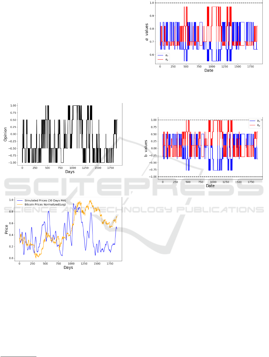
Figure 3: Alpha dynamics applying U

= 0.2, L

= 0.8,

= 0.3, P0

= 0.7. This ﬁgure illustrates the dynamics

of two self-reinforcing parameters, α

(in red) and α

(in

blue), over time. These parameters represent the sensitivity

or reinforcement levels for the Positive Group and Negative

Group, respectively, as they respond to market mood.

Figure 4: Input dynamics applying U

= 0.3, L

= 0.1,

= 0.8, and P0

= 0.1. This ﬁgure shows the dynam-

ics of the input parameters b

(in red) and b

(in blue) over

time, representing external input factors that inﬂuence the

positive group and negative group, respectively.

sentiment are reﬂected in price movements.

Figure 3 illustrates the dynamics of the self-

reinforcing parameters α

and α

over time, cor-

responding to the self-reinforcement of the positive

and negative groups, respectively. When the market

mood is positive, α

tends to increase, which means

the positive group is more self-reinforcing. Con-

versely, when the market mood is negative, α

tends

to rise, meaning that the negative group is more self-

reinforcing. This pattern shows that the values of

α adapt to prevailing market sentiment, altering the

reinforcement of each group’s opinion based on the

overall market mood. However, recall the dynamics

(1) and (2) and since, σ = 1, then the group’s self-

reinforcing parameter α needs to exceed the critical

value, i.e. α > 1 for the group to allow for the posi-

tive feedback α ˆx to dominate. As shown in Figure 3

α values never reach 1, both groups will be more in-

ﬂuenced by each other’s opinions. Hence, σ controls

the tendency to herding.

Figure 4, shows that when the market mood is pos-

itive, the magnitude of input parameter b

for the pos-

ICAART 2025 - 17th International Conference on Agents and Artiﬁcial Intelligence

1128

Figure 5: Opinion evolution for two distinct groups in the

market: a “positive group” (represented in red) and a “neg-

ative group” (in blue). Group opinion dynamics when ap-

plying the optimal parameters setting.

itive group tends to be higher, adding to the group’s

positive opinion. This positive external input aligns

with the market sentiment, strengthening the positive

group’s opinion. Conversely, when the market mood

is negative, the magnitude of input parameter b

for

the negative group increases, adding to the group’s

negative opinion. It can be noted that the positive

group’s input is higher than the negative group’s in-

put.

Figure 5 presents the group opinion dynamics af-

ter applying the optimal parameter settings obtained

from the calibration process and updating agents’

opinions as per equations (1) and (2) accordingly.

This ﬁgure shows how the model, ﬁne-tuned with

these parameters, captures shifts in group opinions

over time, reﬂecting a more realistic and potentially

accurate representation of trader’s group opinions

compared to the baseline. The dynamics here con-

sider interactions and feedback mechanisms that the

optimal parameters enable. Since the negative group

has the lower self-reinforcement and the lower inputs,

I found that the best instances of the model’s evolution

happen when the positive group update their opinion

at a higher rate, which means as the initial opinions

are −1 and +1, for the negative group and the positive

group respectfully, the negative group get to keep its

negative average opinion close to the initial opinion,

and the dynamics in (1) will results in negative opin-

ion. The jump in opinions happens around days 500

or 900 when the positive group becomes more self-

reinforcing (α

> α

) and (α

> 0.9); and receives

more inputs (b

> b

). Thus, x

becomes greater and

updating (2) will give a positive opinion. It is note-

worthy to mention that since the prediction market

expects opinions to be in [−1,+1], opinions need to

be scaled. I use this simple linear transformation that

maps the values of

Figure 6 shows that the market prices resulting

from using the calibrated model capture the general

Figure 6: This ﬁgure shows the simulated average price

from 150 model simulations (blue line) with the actual, nor-

malized Bitcoin price (orange line) over the same time pe-

riod.

upward and downward trends in Bitcoin’s price but

lack some of the high-frequency volatility present in

the actual Bitcoin market. The model provides a good

approximation of the overall trend but may not fully

capture the rapid ﬂuctuations or extreme volatility

seen in real-world cryptocurrency markets. These re-

sults demonstrate the model’s capacity to follow long-

term price movements while highlighting potential ar-

eas for improving its responsiveness to sudden market

shifts.

The distribution of residuals represents the differ-

ences between Bitcoin prices and the simulated prices

generated by the calibrated model. These residuals

are centered around zero, indicating that the model is

not biased. However, the residuals are not perfectly

normally distributed, with a mean of µ = 0.00 and a

standard deviation of σ = 0.16. The skewed spread

and shape of the residuals suggest that the model may

not fully capture the underlying distribution of the

data.

To evaluate the relationship between simulated

prices and Bitcoin prices, Exponential Moving Aver-

ages (EMAs) and residual analysis are applied. First,

EMAs are calculated for both simulated prices and

Bitcoin prices to smooth ﬂuctuations caused by the

high frequency of trading in the simulation. EMAs

are optimized through a minimization process aimed

at reducing the variance of the residuals. After cal-

culating the residuals, zero-crossings—points where

the residuals change sign—are identiﬁed. These zero-

crossings segment the time series into distinct phases,

each representing periods of consistent residual be-

havior. The mean residual for each phase is calcu-

lated to summarize the overall behavior during that

phase. Linear regression is applied to the residuals

within each phase to examine trends. Figure 7 (top)

shows the EMAs for both series, and Figure 7 (bot-

tom) displays the phase means during speciﬁc time

phases alongside the EMA of residuals time series.

Price Drivers in Prediction Markets: An Agent-Based Model of Competing Narratives

1129

Figure 7: Comparison of Exponential Moving Averages

(EMAs) of simulated prices and Bitcoin (BTC) prices. The

top plot shows the EMAs of simulated prices (blue) and Bit-

coin prices (orange) over time, with optimal span values of

50 days for simulated prices and 200 days for Bitcoin prices.

The bottom plot displays the residuals, smoothed using an

EMA with a span of 200 days, calculated as the difference

between the EMAs of simulated prices and Bitcoin prices.

The red dashed lines represent the linear regression of the

residuals, with corresponding means annotated.

In Phase 1 (t

to t

116

), the mean of residuals is

positive (0.094), indicating that simulated prices are

higher than Bitcoin prices. During Phase 2 (t

116

408

), the mean of residuals turns negative (-0.049),

showing that Bitcoin prices are higher. In Phase 3

408

to t

563

), the mean of residuals is slightly posi-

tive (0.023), with simulated prices being higher again.

Phase 4 (t

563

to t

1142

) is characterized by a negative

mean of residuals (-0.097), indicating a pronounced

divergence where Bitcoin prices are much higher. Fi-

nally, in Phase 5 (t

1142

to t

1884

), the mean of resid-

uals becomes positive once more (0.082), showing a

return to simulated prices being higher. On average,

the residuals are close to zero relative to the normal-

ized price scale (0 to 1), suggesting that the model

performs reasonably well. However, during certain

periods, such as Phase 4, the residuals are relatively

larger, indicating that the model’s predictions are less

accurate.

Table 1: Comparison of Performance Metrics for the cali-

brated model and the baseline model.

Metric Calibrated Model Baseline

MSE 0.03 0.12

MAE 0.13 0.29

RMSE 0.16 0.35

R² 0.77 -0.85

Pearson

Correlation

0.88 0.23

Table 1 provides a comparison of the calibrated

model and the baseline model across several perfor-

mance metrics: Mean Squared Error (MSE), Mean

Absolute Error (MAE), Root Mean Squared Error

(RMSE), R-squared (R²), and Pearson Correlation.

The calibrated model shows a signiﬁcant improve-

ment over the baseline in all metrics. With an MSE

of 0.026 compared to 0.124 for the baseline, the cali-

brated model demonstrates more accurate predictions

with smaller average squared deviations from the true

values. Similarly, the MAE is much lower (0.133 for

the calibrated model vs. 0.288 for the baseline), indi-

cating that the predictions are generally closer to ac-

tual values. The RMSE, which gives more weight to

larger errors, is also considerably lower for the cali-

brated model (0.161 versus 0.352), highlighting fewer

large deviations from the actual data.

Additionally, the calibrated model achieves an R-

squared value of 0.772, meaning it explains approx-

imately 77.2% of the variance in the data, while the

baseline model has a negative R-squared, indicating a

poor ﬁt. Lastly, the Pearson Correlation for the cali-

brated model is 0.883, showing a strong positive lin-

ear relationship between the predicted and actual val-

ues, compared to a weaker correlation of 0.230 for

the baseline. Overall, these metrics underscore the

superior accuracy and predictive capability of the cal-

ibrated model over the baseline.

3.3 Financial Market Forecasting

We can use the calibrated parameters from the model

of the prediction market to forecast the ﬁnancial mar-

ket. We can formulate the problem of short-term fore-

casting of asset prices and group opinion dynamics

as multi-target regression (MTR) problem. Formally,

given an input vector X ∈ R

representing the features

—parameter values, market mood and price history—

, the goal is to predict an output vector Y ∈ R

where

each element y

represents the predicted value for a

speciﬁc target variable (e.g., future prices at differ-

ent time horizons), and the expected group dynamics.

This formulation allows us to leverage supervised ma-

chine learning techniques to learn a mapping function

f : R

→ R

such that:

Y = f (X) + ε

where ε denotes a vector of error terms, captur-

ing the model’s prediction error. MTR problems

can be solved by a variety of machine-learning al-

gorithms. Given that the generated dataset contains

targets that are both continuous and categorical, inter-

dependent, and the dataset size is small. It is impor-

tant to use multi-target supervised machine learning

methods that are capable of effectively handling tar-

get interdependencies while at the same time avoiding

overﬁtting due to limited data.

Table 2 presents the performance metrics for sev-

eral multi-target learning algorithms, Multi-Output

ICAART 2025 - 17th International Conference on Agents and Artiﬁcial Intelligence

1130

Random Forest (MORF), a variant of Random For-

est, models interdependencies within tree splits and

is particularly robust for small datasets, making it an

effective choice for multi-target tasks. Extreme Gra-

dient Boosting Trees (XGBoost) support multi-target

prediction and perform exceptionally well on smaller

datasets. Finally, Multi-Task Learning Neural Net-

works (MTNN) leverage shared hidden layers to cap-

ture features common across all targets while utiliz-

ing separate output layers tailored to handle contin-

uous and categorical variables. MTXGBoost gener-

ally achieves the best performance across most tar-

gets, followed closely by MORF, while MTNN shows

slightly higher errors but remains competitive in cer-

tain cases.

Table 2: Performance Metrics for Multi-target Models.

Model Target MAE RMSE R²

MTXGBoost

Price 0.16 0.24 0.86

0.02 0.04 0.82

0.03 0.05 0.77

0.11 0.16 0.84

0.11 0.16 0.83

MORF

Price 0.17 0.25 0.85

0.02 0.04 0.80

0.03 0.05 0.76

0.12 0.16 0.83

0.12 0.17 0.82

MTNN

Price 0.16 0.24 0.86

0.03 0.04 0.76

0.04 0.05 0.70

0.12 0.16 0.83

0.13 0.17 0.82

4 CONCLUSION

In this paper, I explored price formation in prediction

markets, by populating a simple model of a prediction

market exchange with opinionated agents and cali-

brating model parameters. I investigated the inﬂuence

of key drivers in the opinion formation process within

two competing groups: self-reinforcement, herding,

and additive responses to inputs. Using a real-world

dataset, the results indicate that both groups generally

follow overall market sentiment. However, when mar-

ket mood aligns with a particular group’s opinion, that

group becomes more self-reinforcing, while a lack of

alignment reduces self-reinforcement.

Despite these insights, there are limitations to this

simple ABM. The model’s simpliﬁed structure does

not fully capture the complexity of real-world trad-

ing behavior, particularly the high-frequency volatil-

ity and external shocks often observed in cryptocur-

rency markets. Additionally, while the model accu-

rately reﬂects long-term sentiment trends, it may fail

to capture the rapid sentiment shifts that occur in ac-

tual trading environments. Future work could ad-

dress these limitations by incorporating more com-

plex agent interactions or external factors inﬂuenc-

ing market sentiment. Nevertheless, the model in-

troduced here does capture real-world price dynamics

with sufﬁcient accuracy to be of signiﬁcant and endur-

ing interest. To enable other researchers to replicate

and extend this work I have made the source code and

sample data sets available on GitHub.

REFERENCES

Benedetti, M., Catapano, G., Sclavis, F. D., Favorito, M.,

Glielmo, A., Magnanimi, D., and Muci, A. (2022).

Black-it: A ready-to-use and easy-to-extend calibra-

tion kit for agent-based models. Journal of Open

Source Software, 7(79):4622.

Berg, J. E. and Rietz, T. A. (2003). Prediction markets as

decision support systems. Information systems fron-

tiers, 5:79–93.

Bizyaeva, A., Franci, A., and Leonard, N. E. (2020). A

general model of opinion dynamics with tunable sen-

sitivity. arXiv preprint arXiv:2009.04332.

Bizyaeva, A., Franci, A., and Leonard, N. E. (2022).

Nonlinear opinion dynamics with tunable sensitiv-

ity. IEEE Transactions on Automatic Control,

68(3):1415–1430.

Glielmo, A., Favorito, M., Chanda, D., and Delli Gatti, D.

(2023). Reinforcement learning for combining search

methods in the calibration of economic abms. In Pro-

ceedings of the Fourth ACM International Conference

on AI in Finance, pages 305–313.

Leonard, N. E., Keena Lipsitz, Anastasia Bizyaeva, Alessio

Franci, and Yphtach Lelkes (2021). The nonlinear

feedback dynamics of asymmetric political polariza-

tion. Proceedings of the National Academy of Sci-

ences, 118(50):e2102149118.

Luckner, S., Schr

oder, J., Slamka, C., Skiera, B., Spann,

M., Weinhardt, C., Geyer-Schulz, A., and Franke, M.

(2011). Prediction markets: Fundamentals, designs,

and applications. Springer Science & Business Me-

dia.

Restocchi, V., McGroarty, F., Gerding, E., and Brede, M.

(2023). Opinion dynamics explain price formation in

prediction markets. Entropy, 25(8):1152.

Song, B., Xiong, G., Yu, S., Ye, P., Dong, X., and Lv, Y.

(2021). Calibration of agent-based model using rein-

forcement learning. In 2021 IEEE 1st International

Conference on Digital Twins and Parallel Intelligence

(DTPI), pages 278–281. IEEE.

Price Drivers in Prediction Markets: An Agent-Based Model of Competing Narratives

1131