Graph Convolutional Networks and Particle Competition and
Cooperation for Semi-Supervised Learning
Gustavo Rosseto Leticio
a
, Matheus Henrique Jacob dos Santos
b
, Lucas Pascotti Valem
c
,
Vinicius Atsushi Sato Kawai
d
, Fabricio Aparecido Breve
e
and
Daniel Carlos Guimar
˜
aes Pedronette
f
Department of Statistics, Applied Mathematics, and Computing (DEMAC),
S
˜
ao Paulo State University (UNESP), Rio Claro, Brazil
Keywords:
Semi-Supervised Learning, Graph Convolutional Networks, Particle Competition and Cooperation.
Abstract:
Given the substantial challenges associated with obtaining labeled data, including high costs, time consump-
tion, and the frequent need for expert involvement, semi-supervised learning has garnered increased attention.
In these scenarios, Graph Convolutional Networks (GCNs) offer an attractive and promising solution, as they
can effectively leverage labeled and unlabeled data for classification. Through their ability to capture complex
relationships within data, GCNs provide a powerful framework for tasks that rely on limited labeled informa-
tion. There are also other promising approaches that exploit the graph structure for more effective learning,
such as the Particle Competition and Cooperation (PCC), an algorithm that models label propagation through
particles that compete and cooperate on a graph constructed from the data, exploiting similarity relationships
between instances. In this work, we propose a novel approach that combines PCC, GCN, and dimensional-
ity reduction approaches for improved classification performance. The experimental results showed that our
method provided gains in most cases.
1 INTRODUCTION
In computer science, classification tasks have ad-
vanced significantly over the last decade, driven by
diverse approaches and deep learning models. How-
ever, despite these strides, performing classification
with limited labeled data remains an intricate chal-
lenge, as deep models often require extensive data
for training. In this context, semi-supervised learn-
ing (SSL) has emerged as a promising solution, po-
sitioned between supervised and unsupervised meth-
ods, SSL proves effective in handling substantial
amounts of unlabeled data along with a modest quan-
tity of labeled data. A key motivation for adopting
SSL lies in the difficulty in obtaining labeled data,
which is typically more arduous compared to acquir-
ing unlabeled data. SSL techniques are particularly
a
https://orcid.org/0009-0008-3715-8991
b
https://orcid.org/0009-0005-5956-4016
c
https://orcid.org/0000-0002-3833-9072
d
https://orcid.org/0000-0003-0153-7910
e
https://orcid.org/0000-0002-1123-9784
f
https://orcid.org/0000-0002-2867-4838
useful for datasets with limited labeled data due to the
high cost and time required for labeling.
In scenarios with limited labeled data, most super-
vised methods struggle to perform effectively due to
their dependency on extensive labels. SSL overcomes
this limitation by exploiting the underlying structure
of data distributions. It uses labeled data to guide the
learning process while also taking advantage of the
unlabeled data to better understand the latent patterns
present in the dataset (Wang et al., 2024).
Among the diverse techniques employed in SSL,
pseudo-labeling stands out as an intuitive strategy.
Based on the principle of proximity, pseudo-labeling
assumes that an unlabeled instance is likely to share
the same class as its closest labeled neighbor. By as-
signing pseudo-labels to such instances, the method
incorporates unlabeled data into the training process,
gradually enhancing the model’s robustness and gen-
eralization capabilities.
In addition to the various SSL techniques, graph-
based methods, such as Particle Competition and
Cooperation (PCC) and Graph Convolutional Net-
works (GCNs), use graph structures to model rela-
tionships between instances, enhancing learning from
Leticio, G. R., Santos, M. H. J., Valem, L. P., Kawai, V. A. S., Breve, F. A. and Pedronette, D. C. G.
Graph Convolutional Networks and Particle Competition and Cooperation for Semi-Supervised Learning.
DOI: 10.5220/0013267000003912
Paper published under CC license (CC BY-NC-ND 4.0)
In Proceedings of the 20th International Joint Conference on Computer Vision, Imaging and Computer Graphics Theory and Applications (VISIGRAPP 2025) - Volume 2: VISAPP, pages
519-526
ISBN: 978-989-758-728-3; ISSN: 2184-4321
Proceedings Copyright © 2025 by SCITEPRESS – Science and Technology Publications, Lda.
519

labeled and unlabeled data. PCC is an algorithm that
models label propagation through particles that com-
pete and cooperate on a graph constructed from the
data, exploiting similarity relationships between in-
stances (Breve et al., 2012). On the other hand, GCNs
learn node representations by aggregating neighbor-
hood information (Kipf and Welling, 2017). Unlike
traditional classifiers, GCNs require two inputs: fea-
ture representations and a graph that encodes contex-
tual relationships. The graph is fundamental for en-
abling GCNs to consider neighborhood context, en-
hancing their classification capabilities.
Despite their potential, most GCN models are
evaluated on scenarios where the graph is already
available, such as citation datasets (e.g., Cora, Cite-
Seer) (McCallum et al., 2000; Giles et al., 1998). This
limitation highlights the need to develop strategies
that effectively encode similarity information in graph
structures and feature representations.
In this work, we propose a novel approach for
semi-supervised classification that combines the PCC
algorithm with GCNs, integrating dimensionality re-
duction techniques such as t-SNE and UMAP. The
main contributions of this work are:
• Combination of semi-supervised classifiers (PCC
and GCN) with dimensionality reduction ap-
proaches (t-SNE and UMAP) for improving clas-
sification.
• Leverages dimensionality reduction techniques in
conjunction with the semantic embeddings pro-
duced by the PCC classifier to enhance the train-
ing of the GCN model.
• Exploits dimensionality reduction methods to
construct a more effective graph, improving the
training process for both the PCC and GCN clas-
sifiers.
The remainder of this paper is organized as fol-
lows: Section 2 reviews the literature; Section 3
presents the formal notation used along with the pa-
per; Section 4 discusses the proposed approach; Sec-
tion 5 presents the experimental evaluation; Finally,
in Section 6, we discuss the conclusions.
2 RELATED WORK
Recently, (Anghinoni et al., 2023) presented a novel
approach to improving Graph Neural Networks
(GNNs), the Transductive Graph Neural Network
with Graph Dynamic Embedding (TransGNN), which
introduces a new message-passing technique based
on the Particle Competition and Cooperation (PCC)
model, originally designed for community detec-
tion in graphs. Traditional GNNs primarily learn
from data attributes and relationships through mes-
sage passing, but they often face the issue of over-
smoothing, where node representations become in-
distinguishable. TransGNN incorporates a two-step
learning process: first, it performs transductive learn-
ing on the network, using the PCC-based message
passing to propagate learned information to the nodes.
This is followed by the standard inductive learning
used in conventional GNNs. The approach addresses
over-smoothing and demonstrates improved classifi-
cation accuracy, reduced computational cost, and ef-
fective learning with limited labeled data.
Despite the similarities between our approach and
TransGNN, there are key differences in how PCC
and the graph structure are employed. TransGNN
incorporates PCC during the training phase as a
dynamic message-passing mechanism, allowing the
graph structure to evolve throughout the process. In
contrast, our approach constructs the graph using a
reduced representation of the original features. This
graph serves two purposes: it provides the structural
input for the GCN and is used by PCC to generate ad-
ditional features, capturing local and global relation-
ships. Additionally, the original features are reduced
using UMAP, and the UMAP-reduced features are
concatenated with the PCC output to form a combined
feature representation. Unlike TransGNN, which fo-
cuses on dynamic graph adaptation, our method em-
phasizes the integration of dimensionality reduction
techniques and semi-supervised classifiers to enhance
performance in scenarios with limited labeled data.
Recent work in the literature (Benato et al., 2024)
proposed an approach that combines pseudo-labeling
and dimensionality reduction to improve classifica-
tion in scenarios with limited labeled data. Their
methodology leverages 2D projections to capture the
data structure and guide the pseudo-labeling process.
The study demonstrates that high-quality projections
facilitate manual and automatic labeling and con-
tribute to building more robust classifiers by integrat-
ing visualization techniques with active learning.
Our approach diverges from this by employing
a fixed graph structure for GCN training, where di-
mensionality reduction techniques, such as UMAP,
are integrated into the pipeline. The UMAP-reduced
features are combined with additional features gener-
ated through PCC, emphasizing the interplay between
graph-based learning and feature engineering.
In addition, the Optimum-Path Forest (OPF) clas-
sifier (Amorim et al., 2016) has been explored as a
semi-supervised method that iteratively assigns labels
based on confidence.
VISAPP 2025 - 20th International Conference on Computer Vision Theory and Applications
520

3 PROBLEM DEFINITION
In this section, we begin by presenting a formal def-
inition of the semi-supervised learning classification
task based on graphs, largely following the conven-
tions outlined in (Kipf and Welling, 2017; Li et al.,
2018).
Let G represent an undirected graph, defined as
G = (V ,E,X), where V denotes the node set, E rep-
resents the edge set, and X is a feature matrix. The
node set V is given by {v
1
,v
2
,. ..,v
n
}, and the edge
set is defined by pairs (v
i
,v
j
) ∈ E, represented by a
non-negative adjacency matrix A = [a
i j
] ∈ R
n×n
. The
feature matrix X is defined as [x
1
,x
2
,. ..,x
n
]
T
∈ R
n×d
,
where x
i
is a d-dimensional feature vector represent-
ing node v
i
.
Let Y = {y
1
,y
2
,. ..,y
c
} denote a set of labels
assignable to nodes v
i
∈ V . The node set can
be further delineated as {v
1
,v
2
,. ..,v
L
,v
L+1
,. ..,v
n
},
indicating a partially labeled dataset, with V L =
v
i
i = 1
L
representing the labeled subset and V U =
x
i
i = L + 1
n
the unlabeled subset. Typically, in semi-
supervised classification, |V L| ≪ |V U|.
Formally, the training set is seen as a labeling
function l : V
L
→ Y , where y
i
= l(v
i
) for all v
i
∈ V
L
.
The objective is to learn a function
ˆ
l : V
U
→ Y to pre-
dict the labels of unlabeled nodes in V U.
4 PROPOSED APPROACH
This section presents the proposed approach, and is
divided as follows: Section 4.1 provides an overview
of the methodology. In Section 4.2, we discuss the
PCC algorithm. Section 4.3 details the graph con-
struction process. The use of dimensionality re-
duction is explained in Section 4.4. Finally, Sec-
tion 4.5 discusses the Graph Convolutional Networks
(GCNs).
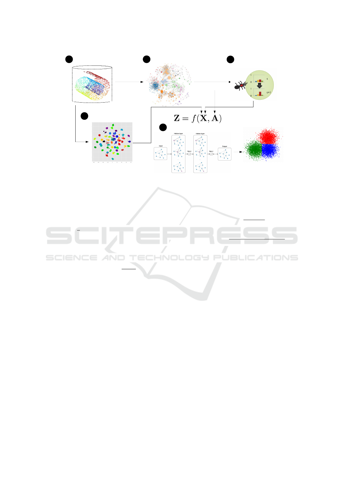
4.1 Overview and Main Ideas
The main idea of the proposed approach is to improve
the effectiveness of semi-supervised classification by
employing a novel workflow that combines the PCC
classifier and dimensionality reduction approaches for
training a GCN model. Figure 1 presents the pro-
posed workflow. Step (A) performs dimensionality
reduction over the original dataset features. Step (B)
builds a kNN graph from the features generated in the
previous step. The PCC classifier is executed in step
(C), which uses the kNN graph as input and gener-
ates a new set of embeddings as output. Step (D)
uses dimensionality reduction (e.g., UMAP or t-SNE)
on the original features and the output is concate-
nated with the PCC features. Finally, step (E) trains
a GCN model considering the concatenated features
from PCC and dimensionality reduction and the kNN
graph generated in (B). The result is the classification
of the elements in the test set.
4.2 Particle Competition and
Cooperation
The semi-supervised learning particle competition
and cooperation (PCC) approach (Breve et al., 2012)
can be outlined as follows. Each node in an undi-
rected and non-weighted graph represents a data item,
and edges connect nodes representing similar data
items. Initially, a particle is assigned to each labeled
node. These particles navigate through the nodes us-
ing a random-greedy strategy, selecting the next node
to visit among the neighbors of the current node. Par-
ticles associated with nodes of the same label form
teams, cooperating to dominate the unlabeled nodes.
Conversely, particles from different teams compete
for control over the nodes.
Each node maintains a set of domination levels,
representing the influence of different teams of par-
ticles. As particles traverse the graph, they increase
their team’s domination level in the visited nodes
while decreasing those of other teams. Ultimately,
each node is labeled based on the team with the high-
est domination level.
In a formal description, for every node v
i
within
the graph G, a particle ρ
i
is instantiated with its ini-
tial position set to v
i
. Each particle ρ
j
possesses a
variable ρ
ω
j
(t) ∈ [0,1], denoting its strength, and de-
termining its influence on the node it visits. Particles
commence with maximum strength, ρ
ω
j
(0) = 1. Ad-
ditionally, each particle ρ
j
maintains a distance table
ρ
d
j
(t) = ρ
d
1
j
(t),ρ
d
2
j
(t),... ,ρ
d
n
j
(t), where each element
ρ
d
i
j
(t) ∈ [0, n − 1] signifies the distance from the
particle’s initial node v
j
to any node v
i
. This distance
table dynamically updates as the associated particle
traverses the graph.
Every node v
i
possesses a domination vector
v
ω
i
(t), with each element v
ω
c
i
(t) ∈ [0,1] representing
the domination level of team/class c over node v
i
. The
total sum of domination levels for each node remains
constant, ensuring that
∑
C
c=1
v
ω
c
i
= 1.
In nodes corresponding to labeled data items,
domination levels remain constant, reflecting com-
plete dominance by the associated class and no influ-
ence from other classes. Conversely, nodes represent-
ing unlabeled data items exhibit variable domination
levels. Initially, all classes’ domination levels are uni-
Graph Convolutional Networks and Particle Competition and Cooperation for Semi-Supervised Learning
521

Parcle
Compeon and
Cooperaon
High-Dimensional
Representaon
Graph Construcon
Neighbors Embedding
Projecon: t-SNE/UMAP
A B
C
D
E
Graph Convoluonal Network
PCA and
Euclidean Distance
kNN Graph
Classi(caon
Figure 1: Our proposed Graph Convolution Networks and Particle Competition and Cooperation for improved classification.
formly set, but these levels are subject to change as
particles visit the nodes. Thus, for each node v
i
, the
domination vector v
ω
i
is initialized as follows:
v
ω
c
i
(0) =



1 if x
i
is labeled and y(x
i
) = c
0 if x
i
is labeled and y(x
i
) ̸= c
1
C
if x
i
is unlabeled
.
(1)
Whenever a particle ρ
j
visits an unlabeled node v
i
,
the node’s domination levels undergo the following
update process:
v
ω
c
i
(t + 1) =







max{0,v
ω
c
i
(t)−
∆
v
ρ
ω
j
(t)
C−1
}
if c ̸= y(ρ
j
)
v
ω
c
i
(t)+
∑
r̸=c
v
ω
r
i
(t)− v
ω
r
i
(t + 1)
if c = y(ρ
j
)
,
(2)
where 0 < ∆
v
≤ 1 is a parameter regulating the rate of
change, and y(ρ
j
) represents the class of particle ρ
j
.
Upon visiting node v
i
, particle ρ
j
adjusts the node’s
domination levels as follows: it elevates the domina-
tion level of its class (v
ω
c
i
where c = y(ρ
j
)) while si-
multaneously reducing the domination levels of other
classes (v
ω
c
i
where c ̸= y(ρ
j
)). Notably, this update
procedure does not apply to labeled nodes, as their
domination levels remain fixed.
The strength of a particle can vary based on the
domination level of its corresponding class at the node
it currently occupies. In each iteration, the parti-
cle’s strength is adjusted according to ρ
ω
j
(t) = v
ω
c
i
(t),
where v
i
denotes the visited node, and c = y(ρ
j
).
During each iteration, a particle ρ
j
selects a node
v
i
to visit from among the neighbors of its current
node. The probability of selecting a node v
i
is deter-
mined by two factors: a) the domination of the parti-
cle’s class on that node, denoted by v
ω
c
i
, and b) the in-
verse of its distance, ρ
d
i
j
. This probability is expressed
as:
p(v
i
|ρ
j
) = (1 − p
grd
)
W
qi
∑
n
µ=1
W
qµ
+ p
grd
W
qi
v
ω
c
i
(1 + ρ
d
i
j
)
−2
∑
n
µ=1
W
qµ
v
ω
c
µ
(1 + ρ
d
µ
j
)
−2
,
(3)
where q is the index of the node being visited by par-
ticle ρ
j
, c is the class label of particle ρ
j
, W
qi
= 1
if there is an edge between the current node and the
node v
i
, and W
qi
= 0 otherwise. After applying (2), a
particle remains on the selected node only if its class
domination level is the highest on that node. Oth-
erwise, a “shock” occurs, prompting the particle to
revert to the previous node and await the next itera-
tion. The parameter p
grd
, ranging between 0 and 1,
controls the balance between randomness and greedi-
ness in the probabilities. A value of 0 implies uniform
probabilities among neighbors, while a value of 1 in-
dicates strong influence from domination levels and
distances.
The algorithm’s termination is based on the sta-
bilization of average maximum domination levels
across nodes, indicating dominance by a single class.
Further details can be found in (Breve et al., 2012).
4.3 Graph Construction
Principal Component Analysis (PCA) (Jolliffe and
Springer-Verlag, 2002) reduces the dimensionality
from the input dataset. Previous work (Breve and Fis-
cher, 2020) has shown that PCC benefits from the use
VISAPP 2025 - 20th International Conference on Computer Vision Theory and Applications
522

of only a few principal components to build its input
graph, instead of all the original dimensions, in most
scenarios. As previously mentioned, the unweighted
and undirected graph is built by representing each
dataset instance as a graph node. Edges connect each
node to its k-nearest neighbors, according to the Eu-
clidean distance among the original data points pro-
jected onto the selected principal components space.
In this paper, the 10 principal components and k = 5
are used throughout all the simulations.
4.4 Neighborhood Embedding
Projection
In general, methods based on neighbor embed-
ding assign probabilities to neighborhood relation-
ships to model attractive and repulsive forces be-
tween neighboring and non-neighboring points in
projections (Ghojogh et al., 2021). This framework
is foundational for non-linear dimensionality reduc-
tion (Damrich et al., 2022) and connects to various
research fields. Two methods have become stan-
dard for visualizing high-dimensional data (Damrich
et al., 2022): t-distributed Stochastic Neighbor Em-
bedding (t-SNE) (van der Maaten and Hinton, 2008)
and Uniform Manifold Approximation and Projection
(UMAP) (McInnes et al., 2018).
The t-distributed stochastic neighbor embedding
(t-SNE) (van der Maaten and Hinton, 2008) is an ex-
tension of the original Stochastic Neighbor Embed-
ding (SNE) technique (Hinton and Roweis, 2002).
SNE is a probabilistic approach aimed at mapping
data into a low-dimensional space while maintain-
ing local neighborhood relationships. It does this by
defining a probability distribution that reflects the po-
tential neighbors in the high-dimensional space and
then approximates this distribution within the low-
dimensional projection. However, t-SNE (van der
Maaten and Hinton, 2008) was specifically devel-
oped to overcome a known optimization issue in SNE,
called the crowding problem. t-SNE’s main innova-
tions include a symmetrized version of the SNE cost
function and the use of a Student’s t-distribution in-
stead of a Gaussian, making the method not only more
straightforward to optimize but also less prone to clus-
tering points too closely together (van der Maaten and
Hinton, 2008).
Uniform Manifold Approximation and Projection
(UMAP) (McInnes et al., 2018) is a manifold learning
technique designed for dimensionality reduction. It is
built upon a sophisticated mathematical foundation,
that includes concepts from manifold theory and topo-
logical data analysis. UMAP exploits local manifold
approximations and fuzzy topological representations
for both high and low-dimensional data. Following
this, it optimizes the projection layout by minimizing
cross-entropy between these topological representa-
tions (McInnes et al., 2018; Ghojogh et al., 2021).
Unlike t-SNE, UMAP is not restricted by the em-
bedding dimension, making it versatile for general-
purpose dimensionality reduction.
Several studies have explored the use of di-
mensionality reduction techniques as a preprocess-
ing step in information retrieval tasks, demonstrating
improvements in data distribution and feature qual-
ity (Leticio et al., 2024; Kawai et al., 2024). In our
approach, we apply these techniques to transform the
original high-dimensional representations into more
compact and informative embeddings, preserving the
proximity relationships among samples.
The resulting embeddings provide a more struc-
tured representation of the data, serving as input to
a GCN. By applying dimensionality reduction before
the GCN, we aim not only to reduce the computa-
tional complexity of the model but also to highlight
relevant structures in the data, facilitating the GCN’s
ability to learn effective representations.
4.5 Graph Convolutional Networks
In recent years, there has been significant interest
in exploiting deep learning techniques for graph-
structured data (Cai et al., 2018). Among these tech-
niques, Graph Convolutional Networks (GCNs), in-
troduced by (Kipf and Welling, 2017), have emerged
as a relevant graph-based neural network model.
GCNs learn node embeddings (representation) by it-
eratively aggregating information from neighboring
nodes, and incorporating the graph structure into the
neural network model. In their first application, a two-
layer GCN model was utilized for semi-supervised
node classification, considering a graph represented
by a symmetric adjacency matrix A.
The network can be formulated as a function of
both the feature matrix X and the adjacency matrix
A: Z = f (X,A), where Z = [z
1
,z
2
,. ..,z
n
]
T
∈ R
n×c
represents the matrix of node embeddings, and each
z
i
is a c-dimensional vector learned for the node v
i
.
As a preprocessing step, the normalized adja-
cency matrix is computed as
ˆ
A =
˜
D
−1/2
˜
A,
˜
D
−1/2
,
where
˜
A = A + I and
˜
D is the degree ma-
trix of
˜
A. Then, the function f (·) which
represents the two-layer GCN model is: Z =
log(so ftmax(
ˆ
AReLU(
ˆ
AXW
(0)
)W
(1)
)).
The matrix W
(0)
∈ R
d×H
defines the neural net-
work weights for an input-to-hidden layer with H fea-
ture maps, while W
(1)
∈ R
H×c
is a hidden-to-output
matrix. Both matrices W
(0)
and W
(1)
are trained us-
Graph Convolutional Networks and Particle Competition and Cooperation for Semi-Supervised Learning
523

ing gradient descent, considering the cross-entropy
error over all labeled nodes v
l
∈ V
L
. The softmax ac-
tivation function is applied row-wise to yield a proba-
bility distribution over the c class labels for each node,
ensuring that the probabilities sum to 1 per node. Fol-
lowing the logarithm function, each node v
i
is as-
signed a label corresponding to the class with the less
negative value in its embedding representation z
i
.
Building on the success of GCNs (Kipf and
Welling, 2017), various related models have been
proposed (Kipf and Welling, 2017; Velickovic et al.,
2018; Klicpera et al., 2019a; Wu et al., 2019; Bianchi
et al., 2019; Li et al., 2018; Bai et al., 2019; Klicpera
et al., 2019b). Some of these models focus on the
structure of network models (Wu et al., 2019; Bianchi
et al., 2019; Klicpera et al., 2019a; Bai et al., 2019),
while others present contributions in training method-
ologies and manifold information (Li et al., 2018;
Klicpera et al., 2019b).
For the node classification task, we used the GCN
by integrating the original features provided by the
datasets with those generated by Particle Competition
and Cooperation (PCC). We constructed the feature
matrix X by concatenating the original features, re-
duced or not in dimensionality through neighborhood
embedding projections (Section 4.4), with the PCC
features, which capture correlations between the data.
This strategy allows the GCN to leverage both the
original features of the data and the correlation infor-
mation provided by PCC.
The adjacency matrix A is obtained from the
graph built by PCC, as detailed in Section 4.3. In this
unweighted and undirected graph, the nodes represent
the dataset instances, and the edges connect each node
to its k nearest neighbors based on the Euclidean dis-
tance of the data points projected onto the principal
components selected by PCA.
It is important to highlight that dimensionality re-
duction methods are used to reduce the dimension-
ality of the original features before their concatena-
tion in the matrix X, while PCA is applied during the
graph construction by PCC.
5 EXPERIMENTAL EVALUATION
In this section, we present the experimental evaluation
of our approach. Section 5.1 describes the datasets
and experimental protocol, followed by parameter
settings in Section 5.2. The results and comparisons
are presented in Section 5.3.
5.1 Datasets and Experimental Protocol
The experimental analysis was conducted on seven
datasets: g241c, g241n, Digit1, USPS, COIL, COIL2,
and BCI. Most datasets contain 1500 points and 241
dimensions, except for BCI, which has 400 points and
117 dimensions. Each dataset has two splits, one split
with 10 labeled points and another with 100.
The majority of these datasets are binary, except
for COIL, which contains 5 classes. COIL2 is a bi-
nary version of COIL. Table 1 summarizes the char-
acteristics of the datasets used in the experiments.
Table 1: Characteristics of the Datasets.
Dataset Points Dimensions Labeled Splits
g241c (set 5) 1500 241 10, 100
g241n (set 7) 1500 241 10, 100
Digit1 (set 1) 1500 241 10, 100
USPS (set 2) 1500 241 10, 100
COIL (set 6) 1500 241 10, 100
COIL2 (set 3) 1500 241 10, 100
BCI (set 4) 400 117 10, 100
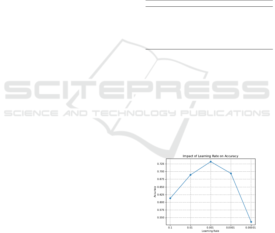
5.2 Parameters Settings
Two parameters were considered regarding parameter
settings: learning rate and number of neurons. The
impact of these parameters was evaluated by varying
its value until a suitable value was found. Figure 2
shows the impact of the learning rate on accuracy.
The tested values were 0.1, 0.01, 0.001, 0.0001, and
0.00001, with the best value being 0.001. Figure 3
presents the evaluation of different numbers of neu-
rons in the hidden layer. The values tested were 16,
32, 48, 64, 80, 96, and 112. The best accuracy was
obtained with 96 neurons.
Figure 2: Impact of learning rate on accuracy.
5.3 Results and Comparisons
This section discusses about the accuracy results of
the proposed approach. Table 2 presents the clas-
sification accuracy across all datasets, each evalu-
VISAPP 2025 - 20th International Conference on Computer Vision Theory and Applications
524

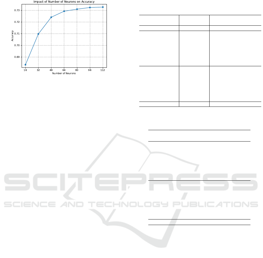
Figure 3: Impact of the number of hidden neurons on accu-
racy.
ated with 10 and 100 labeled instances. The meth-
ods compared include the baseline GCN (Kipf and
Welling, 2017), the Particle Competition and Cooper-
ation (PCC) approach (Breve et al., 2012), and com-
binations of PCC with GCN enhanced by dimension-
ality reduction techniques t-SNE and UMAP.
The results indicate that the combination of PCC,
GCN, and UMAP achieves the highest mean accuracy
(0.7569), outperforming standalone GCN and PCC.
With 10 labeled instances, this approach has the best
accuracy in four datasets, and with 100 instances, it
maintains top performance in most cases.
Additionally, the use of dimensionality reduction
improves GCN’s classification, demonstrating its ef-
fectiveness in enhancing the classification capabili-
ties of GCNs. These findings suggest that combining
PCC with GCN and employing dimensionality reduc-
tion not only leverages structural information from
the graph but also enhances feature representation,
leading to improved classification accuracy.
Furthermore, an evaluation of three GCN mod-
els was considered: GCN (Kipf and Welling, 2017),
SGC (Wu et al., 2019), and APPNP (Klicpera et al.,
2019a). The analysis was done by applying the
proposed approach, with the same parameters and
datasets, in these different models and analyzing the
mean. Table 3 contains the evaluation result. Note
that GCN has better accuracy in most of the cases.
6 CONCLUSIONS
This work proposed a novel approach combining
PCC and dimensionality reduction to improve semi-
supervised classification in GCNs. By applying t-
SNE and UMAP to reduce the original features and
concatenating them with the embeddings generated
by PCC, which uses PCA for graph construction, we
enriched the feature representation fed into GCNs.
Experimental results demonstrated that this combina-
Table 2: Evaluation and comparison of the proposed ap-
proach in different datasets.
Dataset Labeled GCN PCC PCC+ PCC+ PCC+
Set Size GCN GCN GCN
Dim. Reduction - - - t-SNE UMAP
Digit1 10 82.26 88.33 86.77 91.70 91.77
USPS 10 76.96 80.10 77.92 75.09 83.08
COIL2 10 57.43 59.32 57.37 60.81 61.69
BCI 10 51.46 51.04 51.57 50.38 50.56
g241c 10 75.99 72.22 75.89 75.16 73.68
COIL 10 32.22 38.03 32.51 37.46 39.68
g241n 10 72.64 68.65 72.68 71.47 68.76
Digit1 100 95.90 97.19 97.40 97.86 97.61
USPS 100 93.61 94.33 94.19 92.86 94.37
COIL2 100 87.48 91.87 87.37 90.49 92.05
BCI 100 54.32 53.22 54.50 52.44 52.94
g241c 100 81.70 82.36 81.69 82.94 82.82
COIL 100 72.40 81.22 72.84 71.61 80.41
g241n 100 90.56 89.59 90.55 90.08 90.36
Mean - 73.21 74.82 73.80 74.30 75.70
Table 3: Evaluation of different GCN models in combina-
tion with UMAP low-dimensional embeddings.
Dataset Labeled PCC+ PCC+ PCC+
Set Size GCN SGC APPNP
Digit1 10 91.77 69.94 92.31
USPS 10 83.08 71.85 80.64
COIL2 10 61.69 046.7 60.75
BCI 10 50.56 49.97 50.72
g241c 10 73.68 56.62 74.04
COIL 10 39.68 25.75 37.65
g241n 10 68.76 55.45 67.52
Digit1 100 97.61 75.09 97.55
USPS 100 94.37 75.70 93.90
COIL2 100 92.05 67.24 90.75
BCI 100 52.94 50.11 52.58
g241c 100 82.82 68.64 82.86
COIL 100 80.41 36.71 74.84
g241n 100 90.36 66.25 90.31
Mean - 75.70 58.86 74.74
tion outperformed standalone methods, particularly in
scenarios with limited labeled data.
Future work could explore alternative dimension-
ality reduction methods or optimize feature concate-
nation strategies. Applying this approach to datasets
with diverse characteristics would further validate its
robustness and adaptability. Additionally, investigat-
ing alternative graph construction methods may yield
new insights.
ACKNOWLEDGMENT
The authors are grateful to the S
˜
ao Paulo Re-
search Foundation - FAPESP (grant #2018/15597-
6), the Brazilian National Council for Scientific
and Technological Development - CNPq (grants
#313193/2023-1 and #422667/2021-8), and Petro-
bras (grant #2023/00095-3) for their financial support.
This study was financed in part by the Coordenac¸
˜
ao
Graph Convolutional Networks and Particle Competition and Cooperation for Semi-Supervised Learning
525

de Aperfeic¸oamento de Pessoal de N
´
ıvel Superior -
Brasil (CAPES).
REFERENCES
Amorim, W. P., Falc
˜
ao, A. X., Papa, J. P., and Car-
valho, M. H. (2016). Improving semi-supervised learn-
ing through optimum connectivity. Pattern Recognition,
60:72–85.
Anghinoni, L., Zhu, Y.-t., Ji, D., and Zhao, L. (2023).
Transgnn: A transductive graph neural network with
graph dynamic embedding. In 2023 International Joint
Conference on Neural Networks (IJCNN), pages 1–8.
Bai, S., Zhang, F., and Torr, P. H. S. (2019). Hyper-
graph convolution and hypergraph attention. CoRR,
abs/1901.08150.
Benato, B. C., Telea, A. C., and Falcao, A. X.
(2024). Pseudo Labeling and Classification of High-
Dimensional Data using Visual Analytics. PhD thesis,
Utrecht University.
Bianchi, F. M., Grattarola, D., Livi, L., and Alippi, C.
(2019). Graph neural networks with convolutional
ARMA filters. CoRR, abs/1901.01343.
Breve, F. and Fischer, C. N. (2020). Visually impaired aid
using convolutional neural networks, transfer learning,
and particle competition and cooperation. In 2020 Inter-
national Joint Conference on Neural Networks (IJCNN),
pages 1–8. IEEE.
Breve, F., Zhao, L., Quiles, M., Pedrycz, W., and Liu,
J. (2012). Particle competition and cooperation in net-
works for semi-supervised learning. IEEE Transactions
on Knowledge and Data Engineering, 24(9):1686 –1698.
Cai, H., Zheng, V. W., and Chang, K. C. (2018). A com-
prehensive survey of graph embedding: Problems, tech-
niques, and applications. IEEE Trans. Knowl. Data Eng.,
30(9):1616–1637.
Damrich, S., B
¨
ohm, J. N., Hamprecht, F. A., and Kobak,
D. (2022). Contrastive learning unifies t-sne and UMAP.
CoRR, abs/2206.01816.
Ghojogh, B., Ghodsi, A., Karray, F., and Crowley, M.
(2021). Uniform manifold approximation and projection
(umap) and its variants: Tutorial and survey.
Giles, C. L., Bollacker, K. D., and Lawrence, S. (1998).
Citeseer: An automatic citation indexing system. In Pro-
ceedings of the Third ACM Conference on Digital Li-
braries, DL ’98, pages 89–98.
Hinton, G. E. and Roweis, S. (2002). Stochastic neighbor
embedding. In Becker, S., Thrun, S., and Obermayer,
K., editors, Advances in Neural Information Processing
Systems, volume 15. MIT Press.
Jolliffe, I. and Springer-Verlag (2002). Principal Compo-
nent Analysis. Springer Series in Statistics. Springer.
Kawai, V. A. S., Leticio, G. R., Valem, L. P., and Pedronette,
D. C. G. (2024). Neighbor embedding projection and
rank-based manifold learning for image retrieval. In
2024 37th SIBGRAPI Conference on Graphics, Patterns
and Images.
Kipf, T. N. and Welling, M. (2017). Semi-supervised classi-
fication with graph convolutional networks. In 5th Inter-
national Conference on Learning Representations, ICLR
2017, Toulon, France, April 24-26, 2017, Conference
Track Proceedings.
Klicpera, J., Bojchevski, A., and G
¨
unnemann, S. (2019a).
Predict then propagate: Graph neural networks meet
personalized pagerank. In International Conference on
Learning Representations, ICLR 2019.
Klicpera, J., Weißenberger, S., and G
¨
unnemann, S. (2019b).
Diffusion improves graph learning. In Advances in
Neural Information Processing Systems, NeurIPS 2019,
pages 13333–13345.
Leticio, G. R., Kawai, V. S., Valem, L. P., Pedronette, D.
C. G., and da S. Torres, R. (2024). Manifold informa-
tion through neighbor embedding projection for image
retrieval. Pattern Recognition Letters, 183:17–25.
Li, Q., Han, Z., and Wu, X. (2018). Deeper insights into
graph convolutional networks for semi-supervised learn-
ing. In McIlraith, S. A. and Weinberger, K. Q., edi-
tors, Proceedings of the Thirty-Second AAAI Conference
on Artificial Intelligence, (AAAI-18), pages 3538–3545.
AAAI Press.
McCallum, S. K., Nigam, K., Rennie, J., and Seymore, K.
(2000). Automating the construction of internet portals
with machine learning. Information Retrieval, 3:127–
163.
McInnes, L., Healy, J., and Melville, J. (2018). Umap: Uni-
form manifold approximation and projection for dimen-
sion reduction.
van der Maaten, L. and Hinton, G. (2008). Visualizing data
using t-SNE. Journal of Machine Learning Research,
9:2579–2605.
Velickovic, P., Cucurull, G., Casanova, A., Romero, A., Li
`
o,
P., and Bengio, Y. (2018). Graph attention networks.
In 6th International Conference on Learning Represen-
tations, ICLR 2018, Vancouver, BC, Canada, April 30 -
May 3, 2018, Conference Track Proceedings.
Wang, K., Ding, Y., and Han, S. C. (2024). Graph neural
networks for text classification: a survey. Artificial Intel-
ligence Review, 57(8).
Wu, F., Souza, A., Zhang, T., Fifty, C., Yu, T., and Wein-
berger, K. (2019). Simplifying graph convolutional net-
works. In International Conference on Machine Learn-
ing (ICML), volume 97, pages 6861–6871.
VISAPP 2025 - 20th International Conference on Computer Vision Theory and Applications
526