Hybrid Framework for Real-Time Traffic Flow Estimation Using
Breadth-First Search
Sajjad Mahdaviabbasabad
1 a
, Ynte Vanderhoydonc
1 b
, Roeland Vandenberghe
2
and
Siegfried Mercelis
1 c
1
University of Antwerp, imec, IDLab, Faculty of Applied Engineering, Sint-Pietersvliet 7, 2000 Antwerp, Belgium
2
Transport & Mobility Leuven, Diestsesteenweg 71, 3000 Leuven, Belgium
Keywords:
Traffic Flow Estimation, Graph Neural Network, Static Traffic Assignment, Partial Traffic Data Integrity,
Breadth-First Search.
Abstract:
Traffic flow data is essential for urban planning, logistics, transport management, and similar applications.
However, achieving full sensor coverage across a road network is often infeasible due to high installation and
maintenance costs. Simulation data from traffic models can help in filling this gap. However, calibrating
and validating these traffic models is time-consuming. This paper presents a framework that combines real-
time traffic flow predictions from sensor-equipped road segments with 24-hour static simulation data across
an entire network. By applying a method based on the Breadth-First Search algorithm, this framework up-
dates network-wide traffic flow by utilizing the data-driven predictions at sensor-equipped road segments and
simulation data. Evaluation on a network with over 27000 road segments shows that this approach improves
prediction accuracy over static simulation and is viable for real-time deployment.
1 INTRODUCTION
Accurate and timely traffic flow information is essen-
tial for modern transport systems. It enables author-
ities to optimize traffic management, reduce conges-
tion, and improve road safety. With this data, urban
planners and traffic administrators can implement ef-
fective traffic control strategies to enhance transporta-
tion efficiency and reduce environmental impact. Ad-
ditionally, traffic data helps identify congested roads,
manage traffic flow, and support long-term urban
planning for sustainable development.
However, gathering comprehensive traffic data across
an entire network is challenging due to the high cost
of sensor deployment (Zhan et al., 2016) and the
logistical difficulties of maintaining these systems.
Many cities, especially those with large road net-
works, face challenges in deploying sufficient num-
ber of sensors to provide continuous real-time traffic
data. Moreover, traffic data quality is another chal-
lenge, influenced by factors such as the sensor place-
ment, collection frequency, and potential disruptions
during data transmission (Contreras et al., 2017).
To overcome these challenges, many cities rely on
a
https://orcid.org/0009-0006-2566-9802
b
https://orcid.org/0000-0001-6835-3302
c
https://orcid.org/0000-0001-9355-6566
traffic models to simulate flow across areas without
sensors. While these models can provide network-
wide insights, they face their own issues. For in-
stance, these models require extensive traffic data for
parameter calibration and model validation, a process
that is not only time-consuming and labor-intensive
but also prone to errors. Furthermore, because of the
inherent discrepancy between traffic models and real-
time traffic behaviour, these models have limitations
in terms of accuracy and precision in traffic estimation
(Zhang et al., 2024).
In this paper, we propose a framework that ad-
dresses these challenges by combining data-driven
predictions for sensor-equipped segments with static
24-hour simulation flow data for the entire road net-
work in a study area of Antwerp, Belgium. This net-
work consists of over 27000 road segments, of which
only 308 are equipped with sensors for traffic count
measurement. Out of these segments, 194 segments
are located on highways, while the remaining 114 are
in residential areas.
In the proposed framework, we focus on two key steps
to achieve accurate network-wide traffic flow estima-
tion. First, we use a data-driven model to predict traf-
fic flow on sensor-equipped segments. For this, we
employ the Multivariate Time Series Forecasting with
Graph Neural Networks (MTGNN) (Wu et al., 2020),
which is well-suited for capturing complex temporal
Mahdaviabbasabad, S., Vanderhoydonc, Y., Vandenberghe, R. and Mercelis, S.
Hybrid Framework for Real-Time Traffic Flow Estimation Using Breadth-First Search.
DOI: 10.5220/0013271700003941
Paper published under CC license (CC BY-NC-ND 4.0)
In Proceedings of the 11th International Conference on Vehicle Technology and Intelligent Transport Systems (VEHITS 2025), pages 421-430
ISBN: 978-989-758-745-0; ISSN: 2184-495X
Proceedings Copyright © 2025 by SCITEPRESS – Science and Technology Publications, Lda.
421

and spatial relationships in traffic data. Then, we ap-
ply the Breadth-First Search (BFS) algorithm, one of
the most common used graph traversal algorithms and
a building block for various graph applications (Ren
et al., 2022), to propagate these predictions across un-
measured segments and update the flow for the entire
network.
This framework offers several advantages in ad-
dressing key challenges in network-wide traffic flow
estimation. First, by using simulation flow for the
entire network, including both measured and unmea-
sured segments, we address the issue of limited sensor
coverage. Additionally, the use of the MTGNN model
enables us to capture spatial and temporal dependen-
cies within the traffic data, which can enhance the ac-
curacy of predictions on sensor-equipped segments.
Finally, the BFS algorithm efficiently propagates flow
predictions from measured to unmeasured segments,
which not only address the limited sensor coverage is-
sue but also other challenges mentioned earlier. This
allows us to update traffic flow across the entire net-
work by using real-time predictions.
In this study, we aim to evaluate whether use of
the BFS algorithm for propagating flow predictions
across unmeasured segments can outperform static
24-hour simulation data in real-time network-wide
traffic flow estimation.
The paper is organized as follows: Section 2 con-
tains a literature review with a focus on data-driven
and model-driven approaches and their constraints.
Section 3 describes the traffic data. Section 4 out-
lines the methodology behind the proposed frame-
work. The results and discussions are presented in
Section 5. Section 6 concludes and discusses future
work.
2 LITERATURE REVIEW
Traffic prediction has been a key area of research
for many years (Lee and Fambro, 1999), (Williams,
2001), (Kamarianakis and Prastacos, 2003) due to its
important role in traffic management and operations,
such as online vehicle routing and traffic control. Its
importance remains strong, especially with the grow-
ing importance of advanced transportation systems,
including connected and autonomous vehicles (Sun
et al., 2020), as well as adaptive traffic control sys-
tems (Jamil et al., 2022).
In recent years, data-driven approaches have gained
significant attention for their ability to leverage large
volumes of traffic data to enhance prediction accu-
racy. These include deep learning models like GAN
(Goodfellow et al., 2014), CNN (Ma et al., 2017),
and LSTM (Hochreiter, 1997), which are used for
traffic state prediction. Additionally, models like
STGNPP (Jin et al., 2023b), STGCN (Agafonov and
Yumaganov, 2020), DCRNN (Li et al., 2017), MT-
GNN (Wu et al., 2020), and Trafformer (Jin et al.,
2023a) have emerged to further advance the field by
capturing spatial and temporal dependencies in traf-
fic data. For instance, in (Jin et al., 2023a), authors
proposed a model which unified spatial and temporal
information in one transformer-style model.
(Yan et al., 2025) also explored multimodal fusion
techniques for large-scale traffic prediction, demon-
strating how integrating diverse datasets can improve
accuracy. While our study does not explicitly fo-
cus on multimodal data, but incorporating such tech-
niques could enhance the scalability and robustness
of network-wide traffic flow estimation. These neural
network models are particularly effective at adapting
to complex traffic patterns, enabling more accurate
predictions in diverse scenarios. However, to achieve
reliable predictions across large networks, especially
in cities with highly complex traffic patterns, these
models require extensive high-quality data (Fafoutel-
lis and Vlahogianni, 2023), necessitating the deploy-
ment of numerous traffic sensors. This poses a sig-
nificant financial challenge due to the high costs of
sensor installation and maintenance.
Even if sensors are deployed across every road seg-
ment, these models face the additional challenge of
high computational requirements. These models can
be computationally intensive, especially when applied
to large-scale networks, which limits their real-time
deployment (Fafoutellis and Vlahogianni, 2023).
Additionally, these models focus on future traffic state
prediction, aiming to predict the immediate future
values at the specific locations based on the histori-
cal data. However, this paper focuses on estimating
traffic flow at locations without sensors.
Beside the data-driven approach, model-driven
methods provide consistent network-level insights.
However, these models often struggle with capturing
fluctuating daily traffic conditions (Kucharski et al.,
2017). In model-driven approaches, first-order
models, such as Lighthill-Whitham-Richards (LWR)
(Wang et al., 2016), have been widely used to do
traffic state estimation. This has been done by
abstracting physical traffic flow characteristics. As
traffic systems grew more complex, higher-order
models like the Payne-Whitham (PW) (Payne, 1971)
and Aw-Rascle-Zhang (ARZ) (Aw and Rascle, 2000)
were introduced to better represent the dynamic
nature of traffic flow. Despite their simplicity, model-
based methods are often limited by the inherent
constraints of traffic flow models. These methods re-
VEHITS 2025 - 11th International Conference on Vehicle Technology and Intelligent Transport Systems
422

quire extensive data and time-consuming calibration
of parameters, which can be a labor-intensive process
(He et al., 2024).
In summary, while both data-driven and model-
driven approaches have their strengths, these methods
still face some limitations in real-time traffic predic-
tion, especially for large-scale networks. Given these
limitations, a framework is needed that combines the
strengths of both methods to address these issues.
3 DATA DESCRIPTION
3.1 MOW
The “Meten-in-Vlaanderen: minuutwaarden ver-
keersmetingen” dataset provides minute-by-minute
traffic data collected by inductive loop detectors,
mainly on highways in Flanders, provided by
Agentschap Wegen en Verkeer (Agentschap We-
gen en Verkeer, 2023) and Vlaams Verkeerscentrum
(Vlaams Verkeerscentrum, 2023), and denoted as the
MOW dataset. This dataset includes the number of
vehicles, average speeds, and classifications into five
vehicle types. In this paper, we use the MOW data
from the highways around Antwerp, Belgium. These
detectors help us to collect important traffic details
like vehicle counts and speeds. The historical data
is collected from 1 January 2022 to 1 January 2023.
In this study, only the count data is utilized.
3.2 Telraam
The Telraam dataset (Telraam, 2023) provides traffic
data collected through a network of sensors, installed
by citizens which enables real-time traffic monitor-
ing in various locations. These sensors, placed on
the windows overlooking streets and measure vehi-
cle counts, speeds, and distinguish between different
types of road users such as cars, bicycles, pedestrians,
and heavy vehicles. The dataset is updated hourly.
The raw data includes 71 sensors within Antwerp and
the historical datasets, similar as MOW data, has traf-
fic data records from 1 January 2022 to 1 January
2023. These sensors provide detailed vehicle counts
and speed data, divided into measurements for both
directions, recorded separately. Similar to the MOW
dataset, we use only the count data from Telraam in
this study.
3.3 Origin-Destination Matrix
An origin-destination (OD) matrix for the study area
is made available by the Flemish Government for each
hour of a typical working day and for cars, trucks, and
bikes. The methodology used in the strategic traffic
models of the Flemish Government is summarized in
(Vanderhoydonc et al., 2018).
3.4 Counting Campaigns
Manual traffic counts were performed in the study
area during temporary counting campaigns for var-
ious purposes (roadworks, monitoring). The cam-
paigns are typically focused on intersections – where
all turning movements during peak hours on one day
are counted – or on strategically chosen road seg-
ments – where loop counters count traffic for several
weeks. Within the study area, about 400 locations
were counted recently, and we included their counts
to calibrate the traffic assignment model.
As shown in Figure 2, the number of road seg-
ments equipped with sensors is very limited.
4 METHODOLOGY
The primary goal of this study is to leverage the
Breadth-First Search (BFS) method to update the
network-wide flow by integrating predicted traffic
flow from a limited number of road segments (specif-
ically those equipped with MOW and Telraam sen-
sors), derived from data-driven models, into the static
24-hour simulation data available for the entire net-
work.
To achieve this goal, we use three main steps: first,
a data-driven model to predict traffic flow on sensor-
equipped road segments; second, a static traffic as-
signment model to simulate flow across the entire net-
work; and finally, the BFS algorithm to propagate the
predicted flow to the entire road network. Each step
is detailed in the following subsections.
4.1 Data-Driven Model
The first step involves utilizing the MTGNN model to
predict traffic flow on segments equipped with MOW
and Telraam sensors. The MTGNN model archi-
tecture, depicted in Figure 1, includes components
like Graph Learning Layer, Graph Convolutional Net-
works (GCNs) layers, and Temporal Convolutional
Networks (TCNs) Layers. This Architecture pro-
cesses multivariate time series data enhanced with ex-
ternal features. It models spatial relationships using
Hybrid Framework for Real-Time Traffic Flow Estimation Using Breadth-First Search
423

Figure 1: MTGNN model architecture.
Figure 2: Location of sensor data with traffic count mea-
surements highlighted in red on the map of the study area.
GCNs, while TCNs capture temporal patterns. The
Graph Learning Layer dynamically learns the graph
adjacency matrix used by the GCN, enabling effec-
tive processing of historical and real-time traffic data.
This adjacency matrix helps the model understand the
road network layout.
The MTGNN model is separately applied to
MOW and Telraam datasets. In this study, count and
speed values are used from the MOW dataset, while
only count values are used from the Telraam dataset.
The MOW data, recording minute-by-minute traffic
data, is aggregated in 15-minute. For Telraam data,
which has 1-hour time interval, the intervals remain
unchanged. Both models are trained to predict traffic
counts for the next 2 hours.
4.2 Static Traffic Assignment Model
A Static Traffic Assignment (STA) model is built up
and calibrated for the case study. It starts from a
processed network from OpenStreetMap and an ini-
tial hourly demand matrix provided by the Flemish
Government, which are further calibrated using vari-
ous counting data (Telraam, MOW, and others). The
output includes traffic intensities on every link in the
network and the routes between each origin and des-
tination.
This section provides a concise overview of the traffic
model’s characteristics and outputs.
The traffic assignment calculates a stochastic user-
equilibrium (SUE), which is an equilibrium where ev-
ery user takes the route between his origin and desti-
nation for which they experience the lowest costs.
A travel cost is allocated to all streets and inter-
sections in the network. The costs depend on the
travel time in free-flow and on the prevailing traffic
intensity. For streets, this relation is modelled us-
ing a generic Bureau of Public Roads (BPR) func-
tion. For intersections, more detailed cost functions
are added for different types of intersections (sig-
nalized, right-of-way, roundabouts, and more) that
depend on the type of movement made (left turn,
right turn, etc.). While in traditional traffic assign-
ment congestion spillback is unaccounted for, the
traffic model adopts principles similar to the STAQ-
approach (Brederode et al., 2019). This approach re-
sults in a reduction of traffic flows downstream of the
bottleneck and a queue propagating backwards, ap-
plying the node model proposed by (Tamp
`
ere et al.,
2011). Queues costs are added to the network on the
links.
The demand calibration aims to adapt the traf-
fic demand so that the modelled traffic flows bet-
ter comply with the available traffic counts. Counts
on streets and intersections are collected: mainly
from MOW, Telraam, and counting campaigns on ur-
ban intersections. The optimal OD relations are se-
lected for an adaptation of their demand, such that the
squared deviation between modelled flow and counts
is minimized, while constraints prevent large devi-
ations from the initial estimates, following methods
proposed in i.a. (Frederix et al., 2011).
4.3 Breadth-First Search Method
The BFS algorithm is employed to propagate traf-
fic flows within our entire network. The idea is to
propagate traffic flows from locations with measure-
ments. BFS is a method used to search through a tree-
VEHITS 2025 - 11th International Conference on Vehicle Technology and Intelligent Transport Systems
424

like structure by starting at the root and exploring all
nodes at the current depth before moving on to the
nodes at the next depth level. The graph network is
like a tree data structure where there are nodes, and
an edge that connects the nodes. Hence BFS can be
applied on graph networks, but instead of searching
for a particular node, the searching process is contin-
ued until there are no more connecting nodes. Finally,
the spatial relationship of each node is available (Tay
et al., 2023).
A general overview of the BFS method is illustrated
in Figure 3.
ARCHITECTURE OF BREADTH-FIRST SEARCH
1
7
2
3
4
5
6
8
LEVEL 1
LEVEL 3
LEVEL 2
Select a starting node.
Explore connected unvisited nodes.
Mark visited nodes and proceed
to adjacent ones.
Figure 3: Demonstration how BFS explores nodes level by
level, starting from a chosen node and moving through con-
nected, unvisited nodes at each depth.
To effectively apply the BFS algorithm for up-
dating network-wide traffic flow, it is crucial to first
prepare and process the prediction data accurately.
This preparation involves collecting, standardizing,
and aggregating traffic flow predictions from MOW
and Telraam, which provides critical inputs for our
BFS-driven traffic flow analysis. The subsequent sec-
tions detail the systematic steps taken to transform
predicted data into a structured format suitable for ap-
plying BFS to achieve traffic flow propagation across
the network.
4.3.1 Data Preparation and Graph Construction
We gathered traffic data from two predictive models,
MOW (providing 15-minute interval data) and Tel-
raam (providing hourly data), which are presented in
Section 4.1. This data was combined and aggregated
to represent hourly traffic flow.
The next step in leveraging the BFS algorithm in-
volves constructing a directed graph. This graph rep-
resents the traffic network, where nodes correspond to
intersections or endpoints of traffic links, and edges
represent the roads connecting these nodes. Here is
how we set up the graph:
• Graph Initialization: A directed graph G is initial-
ized using the Python library NetworkX.
• Edge Addition: The data prepared in Section
4.3.1 is iterated through. For each record,
the starting point ( f rom node) and endpoint
(to node) of a link are extracted. Each link is
added as a directed edge in the graph. Alongside
the nodes, we also store attributes for each edge:
– initial f low: the simulation traffic flow on that
link, which provides a baseline measurement of
traffic.
– updated: a boolean flag set to false initially, in-
dicating whether the link’s traffic data has been
updated.
– link id: a unique identifier for each link.
The graph consists of 12678 nodes and 27933 edges,
indicating the complexity and scale of this traffic net-
work.
4.3.2 Conservation of Traffic Flow
In traffic network analysis, it is crucial to ensure the
conservation of traffic flow at each intersection. This
step involves storing outgoing traffic data for each in-
tersection in the traffic network:
• Storing Simulation Flows: Traffic flow data is
gathered into a dictionary, where each key repre-
sents a node and the value is a list of traffic flows
to connected nodes.
• Calculating Flow Ratios: For each node, flow ra-
tios are calculated to maintain traffic balance. We
divide the traffic flow to each outgoing link by the
total outgoing traffic from that node. This ratio
calculation ensures that the sum of all outgoing
traffic from a node aligns with the ratio of simula-
tion flows.
R
to node
=
F
to node
F
total from node
(1)
Where:
– R
to node
: is the flow ratio to the destination
node.
– F
to node
: is the flow from the origin flow to des-
tination flow.
– F
total from node
: is the total of all outgoing flows
from the origin node.
By calculating the flow ratios we not only ensure
static traffic flow conservation but also serve it as
the foundational weights for dynamic adjustments
during the flow propagation process. These ra-
tios act as guiding proportions that dictate how
total flows at a node are redistributed to its outgo-
ing links during the EKF updates. By combining
these static ratios with the EKF’s iterative refine-
ment, flows are dynamically adjusted by consid-
ering real-world uncertainties.
Hybrid Framework for Real-Time Traffic Flow Estimation Using Breadth-First Search
425

Figure 4: BFS method used for traffic flow propagation with F the flow from static simulation data, R the ratio and a attributes.
After calculating the static flow ratios, the Extended
Kalman Filter (EKF) (Kim et al., 2018) is applied as
an additional step. The EKF is applied iteratively dur-
ing the flow propagation through the network. This it-
erative process is important to consider dynamic inter-
dependencies in traffic network, where adjustments in
one part of the network transmit to neighboring nodes.
Initially, the segments with predicted flow values are
updated. By using the calculated ratio, the EKF iter-
atively adjusts flow values by redistributing total out-
going and incoming flows at each node, ensuring that
the propagated flows stay accurate and follow conser-
vation laws.
The EKF dynamically adjusts the flow values
through an iterative process consisting of two key
steps:
Estimation Step:
The estimated flow is calculated as
ˆ
F
t
= R · F
from node
where:
• R: Flow ratio based on static conservation.
• F
from node
: Total incoming flow to the node.
Update Step:
The updated flow is calculated as F
updated
=
ˆ
F
t
+ K ·
(F
initial
−
ˆ
F
t
) where the Kalman gain is given by K =
P
P+R
noise
where:
• P: Estimation uncertainty.
• R
noise
: Measurement noise covariance.
The uncertainty is updated iteratively as
P = (1 − K) · P + Q where Q represents process
noise covariance.
The parameters P
initial
= 2.7, Q = 0.1, and R = 2.8
are determined empirically through experimentation.
We observed that results are moderately sensitive to
changes in P, Q, and R. These values are chosen to
balance the stability of estimations and the adaptabil-
ity of the EKF to changing traffic conditions. Fu-
ture work could explore on identifying their optimal
values through systematic optimization techniques to
fine-tune these parameters based on varying traffic
conditions.
The iteration process allows to refine estimations
over multiple passes, which stabilize flows across the
network and align them with real-world traffic behav-
ior.
4.3.3 Initializing the BFS Algorithm with Traffic
Predictions
To start the BFS algorithm, we first initialize a queue
to manage the nodes that need processing based on
initial traffic predictions. Here’s how it’s set up:
• Queue Initialization: We create a queue to hold
the nodes for which we have predicted traffic flow
data.
• Populating the Queue: We iterate through the traf-
fic data, focusing on entries with non-null pre-
dicted flows. For each valid entry, we check if
there is a corresponding edge in the graph be-
tween the from node and to node. If the edge ex-
ists, we update it with the predicted flow and mark
it as updated. We then add the edge to our queue
for further processing. If it does not exist, we out-
put a message indicating that the initial edge is
missing in the graph.
This step is important as it seeds the BFS algo-
rithm with initial data points which allows for a more
focused and efficient analysis of traffic flow across the
network. The use of a queue helps in systematically
processing each node and ensuring all relevant traffic
data are considered in the simulation.
VEHITS 2025 - 11th International Conference on Vehicle Technology and Intelligent Transport Systems
426

4.3.4 Applying BFS Algorithm to Iteratively
Propagate Flow
• Initialization: set up a queue with nodes that have
direct flow predictions. Each predicted flow is as-
signed to its representative edge in the graph if it
exists.
• Propagation Process:
– Backward Propagation: The algorithm pro-
cesses the queue for backward propagation.
For each node, it calculates the total outgoing
flow and updates the flows of incoming links
to ensure consistency and conservation of flow
throughout the network. The EKF is also ap-
plied to refine these updates based on Kalman
filter parameters.
– Forward Propagation: The algorithm processes
the queue for forward propagation. It calcu-
lates the total incoming flow for each node and
distributes this flow to outgoing links based on
predefined ratios. The EKF again applies the
Kalman filter to refine the flow values.
• Iteration Control: the process iterates through the
graph for a specified number of times (default is
3 iterations, determined by trial and error), recal-
culating and updating flows to stabilize the traffic
pattern across the network.
• Result Compilation: after the iterations, the up-
dated flows are compiled into a dataset.
Figure 4 illustrates the architecture of the BFS
method, detailing the step by step process from data
preparation to flow propagation. In the graph, nodes
(A, B, C, etc.) represent intersections, while edges
(lines connecting nodes) represent the roads or links.
Each edge is associated with attributes: F (the flow
from static simulation data), R (the ratio calculated
for flow distribution), and a (attributes like identifier).
The updated flow F
′
is derived after applying pre-
dictions and propagating them through the network.
In this study, the propagation process was iterated
3 times to ensure the network flow reached a stable
state.
It is important to note that in this study, the order of
adding links to the queue was not specifically con-
sidered, and the process was performed without any
particular ordering. However, exploring the impact of
link order on the results could be an interesting direc-
tion for future work, as it may affect the propagation
process and final traffic flow estimation.
4.4 Performance Evaluation
To Evaluate the performance of this framework, two
error metrics are calculated. First, the Mean Absolute
Error (MAE) is calculated, which is the most pop-
ular error metric, because it gives a straightforward
estimate of the accuracy of the model, as it has the
same unit of measurement as the observation value.
And, the Symmetric Mean Absolute Percentage Er-
ror (SMAPE), which provides a symmetric measure
of estimation accuracy.
MAE =
1
n
n
∑
i=1
|
E
i
− Y
i
|
(2)
SMAPE =
1
n
n
∑
i=1
|
E
i
− Y
i
|

|
Y
i
+E
i
|
2

× 100 (3)
Where:
• Y
i
: Actual observed traffic flows.
• E
i
: Estimated traffic flows.
5 RESULTS AND DISCUSSIONS
The BFS algorithm is tested from 2022-10-20 to
2022-12-31. Since ground truth data is unavail-
able for all road segments, a random masking ap-
proach was applied to segments with ground truth
data. Masking was performed at 20%, 40%, 60% and
80%, removing predicted traffic flow from randomly
selected segments to ensure the BFS method does not
use these predictions during flow propagation.
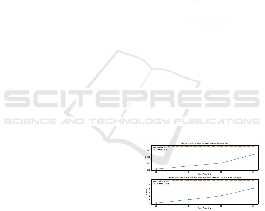
Figure 5: MAE and SMAPE values comparing ground truth
with BFS flow (blue) and Simulation flow (orange) across
varying mask levels (20%, 40%, 60%, 80%).
There are several ways to evaluate the use of the
BFS method. For masked nodes, we can compare
with the ground truth values in the test set. Further-
more, we can compare the estimated values of the
BFS method with a method that would use static sim-
ulation data. The latter on its own can also be com-
pared to the ground truth.
Hybrid Framework for Real-Time Traffic Flow Estimation Using Breadth-First Search
427

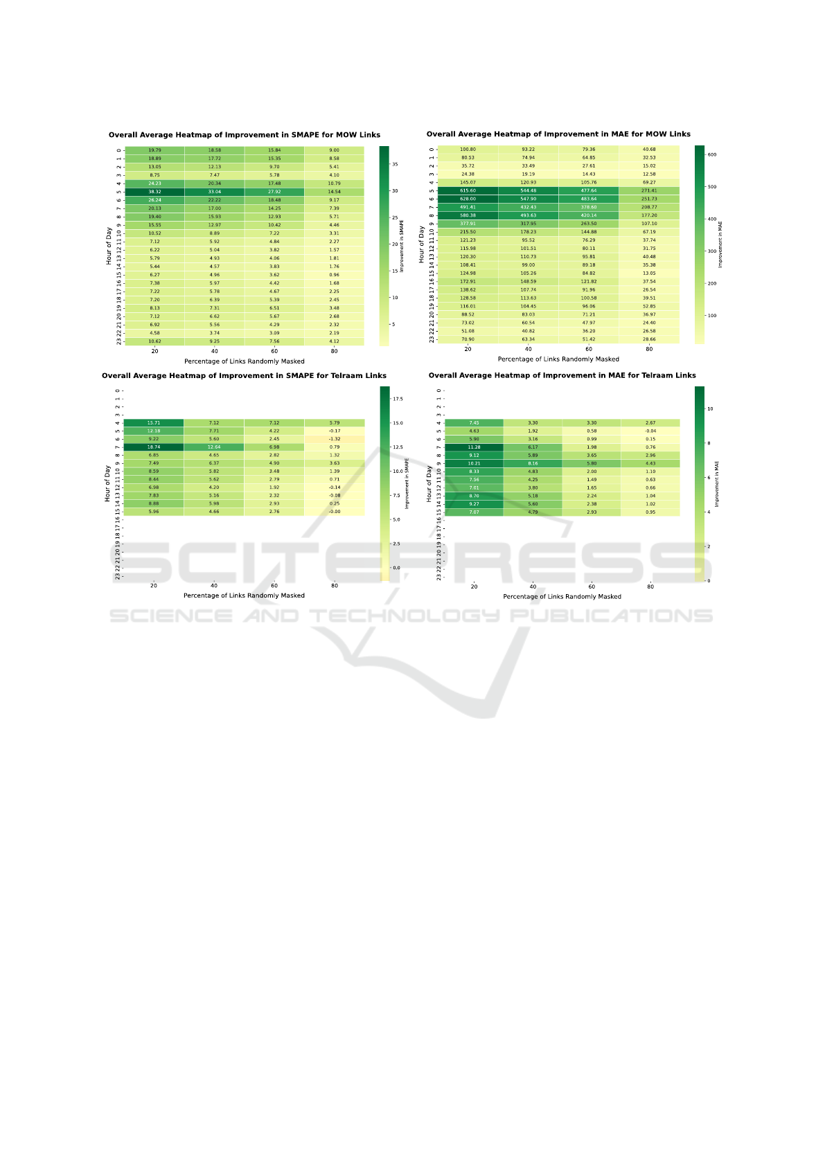
Figure 6: Average SMAPE and MAE improvements across all road segments of MOW and Telraam links over the entire hour
of the day. A random percentage of road segments, ranging from 20% to 80%, were masked to evaluate BFS performance.
Figure 5 observes how MAE and SMAPE evolve
as the percentage of masked predicted data increases.
The BFS flow consistently outperforms simulation
flow across all masking levels, although performance
decreases with higher masking. This highlights the
importance of accurate predicted data from data-
driven models for segments with measurements.
As shown in Figure 6, heatmaps illustrate the aver-
age improvement of BFS over static simulation data.
This improvement is calculated as the difference in
SMAPE and MAE between static simulation data and
BFS results compared to the ground truth, computed
over 24 hours across all masking levels.
Positive values indicate a reduction in error when
BFS is applied.
The formulas used to calculate the improvements
are as follows:
∆SMAPE = SMAPE
GT-Sim
− SMAPE
GT-BFS
(4)
∆MAE = MAE
GT-Sim
− MAE
GT-BFS
(5)
Where:
• ∆SMAPE: Represents improvement in SMAPE.
• ∆MAE: Represents improvement in MAE.
• SMAPE
GT-Sim
: SMAPE between the ground truth
and the static simulation flow.
• SMAPE
GT-BFS
: SMAPE between the ground truth
and the updated flows from the BFS method.
Improvements observed in the highway plots
(MOW dataset) show consistent enhancement across
the 24-hour period, even after applying masking. This
improvement is particularly pronounced during the
morning peak hours.
This improvement is due to the model’s higher accu-
racy in predicting traffic during these times compared
to static simulation flows. Since the BFS method uses
data-driven model predictions, it leads to this substan-
tial improvement.
The same assessment was applied to the Telraam
dataset. Notably, Telraam devices are light-sensitive
and mainly provide data during daytime. At night,
only the latest device versions deliver high-quality
data, which was not included in this study.
VEHITS 2025 - 11th International Conference on Vehicle Technology and Intelligent Transport Systems
428

Figure 6 demonstrates consistent improvement
across all hours and masking percentages, reinforcing
the method’s effectiveness despite varying data avail-
ability.
Furthermore, the BFS method ensures that inflows
and outflows are properly aligned with traffic con-
servation principles. By accurately distributing flow
across the network, especially at key intersections,
it avoids unrealistic discrepancies and ensures traf-
fic patterns follow established principles, leading to
a more reliable representation of real-world behavior.
Table 1: Average MAE and SMAPE errors across different
data mask levels.
Mask level (%) MAE
GT-BFS
SMAPE
GT-BFS
MAE
GT-Sim
SMAPE
GT-Sim
20 251.68 38.07
417.40 50.36
40 274.10 39.94
60 294.77 41.92
80 358.18 46.08
As shown in Table 1, as the masking percentage
increases, the improvement in the updated flow from
the BFS method decreases. This reduction in perfor-
mance is directly related to the decrease in available
road segments equipped with sensors, which results
in fewer predictions across road segments. However,
even in the masked segments, where predictions were
unavailable, the BFS method still demonstrated an
ability to enhance static simulation data which proves
its robustness.
6 CONCLUSIONS & FUTURE
WORK
In this study, we introduced a new framework that
leverages BFS algorithm to propagate traffic flow pre-
dictions throughout the road network, including seg-
ments without sensors. In this framework we inte-
grated traffic flow predictions from MTGNN model
which applied to road segments with sensor data, with
24-hour static simulation flow data derived from a
static traffic assignment model. The overall goal was
to estimate the traffic flow of all the road network in
real-time by combining dynamic data-driven predic-
tions with static simulation flows. This method al-
lowed us to systematically propagate predicted flows
from sensor-equipped segments and ensured all the
traffic data of the static simulation was considered.
Additionally, we maintained the consistency at in-
tersections to ensure balanced inflows and outflows
across the road network.
Based on the performance evaluations which was
done in this study, we can conclude that using this
framework significantly improves the accuracy of es-
timated flows for segments without sensors, which
can address the challenge of calibrating traffic assign-
ment models in real-time which is typically computa-
tionally intensive and time-consuming.
Although this framework shows significant improve-
ments, its accuracy is closely tied to the number of
available sensors. We showed this by our tests with
varying masking level from 20% to 80%. As sensor
coverage decreased, the accuracy of estimated flows
decreased as well. This highlights the importance of
sensor availability for better estimation.
Future research could focus on improving this frame-
work by incorporating dynamic updates to the 24-
hour static simulation data instead of using it as a
fixed dataset. We expect that this improvement can re-
duce the error rates by continuously adapting to real-
time traffic changes. Several other aspects can be ex-
plored in future work. For instance, in the current
study, the effect of link order in the queue was not
specifically considered, and links were added without
a predefined order. Investigating its impact in future
work could provide valuable insights. Additionally,
our results indicate moderate sensitivity to changes
in P, Q, and R. In this study, the values were se-
lected empirically to balance estimation stability, but
future studies could explore systematic optimization
techniques to determine their optimal values based on
varying traffic conditions.
ACKNOWLEDGEMENTS
This research is funded by the imec.icon project Op-
tiRoutS. The imec.icon project OptiRoutS is a re-
search project bringing together academic researchers
and industry partners. The project is co-financed
by imec and receives financial support from Flan-
ders Innovation & Entrepreneurship (project nr.
HBC.2022.0096).
REFERENCES
Agafonov, A. and Yumaganov, A. (2020). Spatio-temporal
graph convolutional networks for short-term traffic
forecasting. In 2020 International Conference on In-
formation Technology and Nanotechnology (ITNT),
pages 1–6. IEEE.
Agentschap Wegen en Verkeer (2023). Agentschap wegen
en verkeer. http://www.wegenenverkeer.be. Accessed:
2023.
Hybrid Framework for Real-Time Traffic Flow Estimation Using Breadth-First Search
429

Aw, A. and Rascle, M. (2000). Resurrection of” second
order” models of traffic flow. SIAM journal on applied
mathematics, 60(3):916–938.
Brederode, L., Pel, A., Wismans, L., de Romph, E., and
Hoogendoorn, S. (2019). Static traffic assignment
with queuing: model properties and applications.
Transportmetrica A: Transport Science, 15(2):179–
214.
Contreras, S., Agarwal, S., and Kachroo, P. (2017). Quality
of traffic observability on highways with lagrangian
sensors. IEEE Transactions on Automation Science
and Engineering, 15(2):761–771.
Fafoutellis, P. and Vlahogianni, E. I. (2023). Unlocking
the full potential of deep learning in traffic forecast-
ing through road network representations: A critical
review. Data Science for Transportation, 5(3):23.
Frederix, R., Viti, F., Corthout, R., and Tamp
`
ere, C. M.
(2011). New gradient approximation method for dy-
namic origin–destination matrix estimation on con-
gested networks. Transportation Research Record,
2263(1):19–25.
Goodfellow, I., Pouget-Abadie, J., Mirza, M., Xu, B.,
Warde-Farley, D., Ozair, S., Courville, A., and Ben-
gio, Y. (2014). Generative adversarial nets. Advances
in neural information processing systems, 27.
He, Y., An, C., Jia, Y., Liu, J., Lu, Z., and Xia, J. (2024).
Efficient and robust freeway traffic speed estimation
under oblique grid using vehicle trajectory data. IEEE
Transactions on Intelligent Transportation Systems.
Hochreiter, S. (1997). Long short-term memory. Neural
Computation MIT-Press.
Jamil, A. R. M., Ganguly, K. K., and Nower, N. (2022). An
experimental analysis of reward functions for adaptive
traffic signal control system. In Distributed Sensing
and Intelligent Systems: Proceedings of ICDSIS 2020,
pages 513–523. Springer.
Jin, D., Shi, J., Wang, R., Li, Y., Huang, Y., and Yang, Y.-B.
(2023a). Trafformer: unify time and space in traffic
prediction. In Proceedings of the AAAI Conference on
Artificial Intelligence, volume 37, pages 8114–8122.
Jin, G., Liu, L., Li, F., and Huang, J. (2023b). Spatio-
temporal graph neural point process for traffic con-
gestion event prediction. In Proceedings of the AAAI
Conference on Artificial Intelligence, volume 37,
pages 14268–14276.
Kamarianakis, Y. and Prastacos, P. (2003). Forecasting traf-
fic flow conditions in an urban network: Compari-
son of multivariate and univariate approaches. Trans-
portation Research Record, 1857(1):74–84.
Kim, Y., Bang, H., et al. (2018). Introduction to kalman
filter and its applications. Introduction and Implemen-
tations of the Kalman Filter, 1:1–16.
Kucharski, R., Kostic, B., and Gentile, G. (2017). Real-
time traffic forecasting with recent dta methods. In
2017 5th IEEE International Conference on Models
and Technologies for Intelligent Transportation Sys-
tems (MT-ITS), pages 474–479. IEEE.
Lee, S. and Fambro, D. B. (1999). Application of subset
autoregressive integrated moving average model for
short-term freeway traffic volume forecasting. Trans-
portation research record, 1678(1):179–188.
Li, Y., Yu, R., Shahabi, C., and Liu, Y. (2017). Diffusion
convolutional recurrent neural network: Data-driven
traffic forecasting. arXiv preprint arXiv:1707.01926.
Ma, X., Dai, Z., He, Z., Ma, J., Wang, Y., and Wang, Y.
(2017). Learning traffic as images: A deep convo-
lutional neural network for large-scale transportation
network speed prediction. sensors, 17(4):818.
Payne, H. J. (1971). Model of freeway traffic and control.
Mathematical Model of Public System, pages 51–61.
Ren, H., Deng, J., Zhang, B., Ye, Z., and Fu, X. (2022).
A breadth-first search algorithm accelerator based on
csci graph data format. pages 636–640.
Sun, C., Guanetti, J., Borrelli, F., and Moura, S. J. (2020).
Optimal eco-driving control of connected and au-
tonomous vehicles through signalized intersections.
IEEE Internet of Things Journal, 7(5):3759–3773.
Tamp
`
ere, C. M., Corthout, R., Cattrysse, D., and Immers,
L. H. (2011). A generic class of first order node
models for dynamic macroscopic simulation of traffic
flows. Transportation Research Part B: Methodologi-
cal, 45(1):289–309.
Tay, L., Lim, J. M.-Y., Liang, S.-N., Keong, C. K., and
Tay, Y. H. (2023). Urban traffic volume estimation
using intelligent transportation system crowdsourced
data. Engineering Applications of Artificial Intelli-
gence, 126:107064.
Telraam (2023). Telraam. https://telraam.net/. Accessed:
2023.
Vanderhoydonc et al. (2018). Strategische verkeersmod-
ellen vlaanderen versie 4.1.1 – overzichtsrap-
portage. https://assets.vlaanderen.be/image/upload/
v1625826383/1
spm 4.1.1 overzichtsrapport tusvju.
pdf.
Vlaams Verkeerscentrum (2023). Vlaams verkeerscentrum.
http://www.verkeerscentrum.be. Accessed: 2023.
Wang, R., Fan, S., and Work, D. B. (2016). Efficient mul-
tiple model particle filtering for joint traffic state es-
timation and incident detection. Transportation Re-
search Part C: Emerging Technologies, 71:521–537.
Williams, B. M. (2001). Multivariate vehicular traffic flow
prediction: evaluation of arimax modeling. Trans-
portation Research Record, 1776(1):194–200.
Wu, Z., Pan, S., Long, G., Jiang, J., Chang, X., and Zhang,
C. (2020). Connecting the dots: Multivariate time se-
ries forecasting with graph neural networks. In Pro-
ceedings of the 26th ACM SIGKDD international con-
ference on knowledge discovery & data mining, pages
753–763.
Yan, Y., Cui, S., Liu, J., Zhao, Y., Zhou, B., and Kuo, Y.-
H. (2025). Multimodal fusion for large-scale traffic
prediction with heterogeneous retentive networks. In-
formation Fusion, 114:102695.
Zhan, X., Zheng, Y., Yi, X., and Ukkusuri, S. V. (2016).
Citywide traffic volume estimation using trajectory
data. IEEE Transactions on Knowledge and Data En-
gineering, 29(2):272–285.
Zhang, J., Mao, S., Yang, L., Ma, W., Li, S., and Gao,
Z. (2024). Physics-informed deep learning for traf-
fic state estimation based on the traffic flow model
and computational graph method. Information Fusion,
101:101971.
VEHITS 2025 - 11th International Conference on Vehicle Technology and Intelligent Transport Systems
430