Routing and Charge Planning Strategies for Ridesharing EV Fleets

Ashutosh Singh and Arobinda Gupta

Dept. of Computer Science & Engineering, Indian Institute of Technology Kharagpur, WB-721302, India

Keywords:

Electric Vehicle, Ridesharing Fleet, Request Assignment, Charge Scheduling.

Abstract:

Ridesharing systems have become an important part of urban transportation. At the same time, electric vehicle

(EV) adoption is also growing at a fast pace as an eco-friendly and sustainable transportation option. To operate

a ridesharing system with EV ﬂeets, scheduling an EV ﬂeet to serve passenger requests requires consideration

of both the requests, and the available charge and potential future charge requirements of the EVs. In this

paper, we address the problem of scheduling EVs by a ridesharing operator, and propose four algorithms

that schedule passenger requests while taking into consideration charging requirements of the EVs. Detailed

simulation results are presented on a real world data set to show that the algorithms perform well.

1 INTRODUCTION

Ridesharing systems have become an important part

of urban transportation, providing on-demand, conve-

nient, and accessible transportation services to pas-

sengers, reshaping the way people move within cities.

Within this evolving landscape, Electric Vehicle (EV)

ﬂeets can play a pivotal role offering a sustainable and

eco-friendly solution to meet the demands of rideshar-

ing. An EV ﬂeet is a collection of electric vehicles

that are owned, operated, or managed by a single cen-

tral entity such as a ridesharing service operator.

A ridesharing operator receives passenger re-

quests for rides and schedules vehicles under its con-

trol based on different criteria/constraints. In compar-

ison to a ﬂeet of non-EV vehicles, scheduling an EV

ﬂeet should consider both passenger requests, and the

current available charge and potential future charge

requirements of the EVs. As the operator controls all

the EVs, it can have complete knowledge about the

EVs at any point in time, which includes their loca-

tion, current charge levels etc. This can allow the op-

erator to plan routes and manage charging schedules

of the EVs more efﬁciently, leading to lower operating

costs. The focus of this paper is addressing the prob-

lem of scheduling passenger requests by a ridesharing

operator with EV ﬂeet while considering the charging

needs of the EVs under different constraints.

The problem addressed can be divided into two

parts, the assignment of EVs to passenger requests,

and scheduling the charging of EVs at appropriate

charging stations at appropriate times. The ﬁrst part

of the problem closely resembles the Vehicle Routing

Problem (VRP), a well-studied optimization problem

in logistics and several works have addressed differ-

ent variants of the problem. Mor et al. (Mor and

Speranza, 2020) provide a comprehensive survey of

the existing works on the vehicle routing problem.

Similarly, the ﬂeet charging problem has also been

investigated, Ma et al. (Ma and Fang, 2022) pro-

vide a survey of the recent developments in this area.

However, there has been very little work at the inter-

section of these two problems. Solving the EV ﬂeet

scheduling problem with passenger requests needs to

consider both – the aspect of vehicle assignment and

routing, and the aspect of charge scheduling. The

few works that have addressed both these issues si-

multaneously (Lu et al., 2012; Chen et al., 2018;

Zalesak and Samaranayake, 2021; Yu et al., 2021)

mostly formulate the problem as a mixed-integer lin-

ear programming (MILP) problem and use optimiza-

tion solvers to solve the problem, or use a reinforce-

ment learning approach. These approaches have an

exponential time complexity in terms of the problem

size, and only work when the problem size (number

of EVs, requests, etc.) is small, thus making these

approaches non-scalable. Also, most of these works

solve the ofﬂine version of the problem, and have ex-

plored a limited set of objective functions.

In this paper, we address the problem of assign-

ing EVs to passenger requests while taking into con-

sideration the charge availability and charging needs

of the EVs. We propose an entirely algorithmic ap-

proach to the two parts of the online version of the

Singh, A. and Gupta, A.

Routing and Charge Planning Strategies for Ridesharing EV Fleets.

DOI: 10.5220/0013282100003941

Paper published under CC license (CC BY-NC-ND 4.0)

In Proceedings of the 11th International Conference on Vehicle Technology and Intelligent Transport Systems (VEHITS 2025), pages 76-87

ISBN: 978-989-758-745-0; ISSN: 2184-495X

problem, exploring new objective functions. In par-

ticular, we propose two strategies each for assigning

passenger requests to EVs and for scheduling EVs

for charging, and consequently, four algorithms using

their combination for the overall problem addressed

that tries to maximize the number of requests served.

Detailed simulation results are presented on a real-

world dataset to show that the algorithms perform

quite well.

The rest of the paper is organized as follows. Sec-

tion 2 provides a brief overview of related works in

the area. Section 3 presents the formal deﬁnition of

the problem. Section 4 presents the proposed algo-

rithms. Detailed simulation results are shown in Sec-

tion 5. Finally, Section 6 concludes the paper.

2 RELATED WORKS

The problem of charging EV ﬂeets have been exten-

sively investigated, both in the area of planning the

charging infrastructure (the number and location of

charging stations, size of EV ﬂeet, charging station

equipment, etc.) (H

all et al., 2018; Zhang et al., 2020;

Schiffer and Walther, 2018; Guo et al., 2021; She-

hadeh et al., 2021; Wu et al., 2021), location-routing

optimization (Schiffer and Walther, 2017; Hua et al.,

2019; Stumpe et al., 2021; Ma and Xie, 2021), and

operational planning such as making decisions on

vehicle routes, charging time and place, amount of

charge etc. (Chen et al., 2016; Zalesak and Sama-

ranayake, 2021; Wang et al., 2018; Lin et al., 2021;

Shi et al., 2020; Guo and Xu, 2022; Lin et al., 2018;

Kullman et al., 2022).

In the area of EV ﬂeet charging while serving pas-

senger requests, which is the focus of this paper, Lu

et al. (Lu et al., 2012) introduce a dispatching policy

designed to optimize electric taxi operations by fac-

toring in taxi demand, the state of charge of electric

taxis, and the presence of battery charging/switching

stations. The primary goal is to minimize recharg-

ing waiting times, ultimately increasing the number

of working hours for taxi drivers. Chen et al. (Chen

et al., 2018) develop a mathematical model to ad-

dress the optimal routing and charging of EV ﬂeets

within a road network, considering factors such as EV

charging rates, charging costs, and state-of-charge re-

quirements. The primary objective is to minimize a

weighted combination of route distances, travel times,

and charging expenses while ensuring that all passen-

ger requests are met. Zalesak et al. (Zalesak and

Samaranayake, 2021) focus on an online electric ve-

hicle ride-sharing system, where real-time customer

requests arrive with speciﬁc entry times, origins, and

destinations. The primary objective was to minimize

the cost of accommodated trips while penalizing un-

served requests. Yu et al. (Yu et al., 2021) tackle

the dynamic optimization problem of maximizing to-

tal proﬁt in a vehicle dispatching system by consid-

ering various factors such as customer requests, EV

charging rates, and penalties for dispatching time and

delays. The primary objective is to determine optimal

vehicle dispatching, relocation, and recharging deci-

sions to maximize revenue while minimizing penal-

ties. As observed earlier, these works are not scal-

able to large number of EVs and requests, and most

of these works solve the ofﬂine version of the prob-

lem.

3 PROBLEM FORMULATION

We consider a city with a set of ﬁxed charging sta-

tions located at speciﬁc locations in the city, where a

ridesharing service operator operates a ﬂeet of EVs to

service passenger requests. The total duration of op-

eration (for example, from 6 am to 8 pm in a day etc.)

is broken up into T time instants. The road network in

the city is modeled as a directed graph G = (N , A),

where N denotes the set of vertices or nodes, and A

is the set of edges (roads between nodes). The nodes

can be charging stations, pickup or dropoff locations,

or other geographical locations of relevance. The dis-

tance between two nodes i and j is denoted by d(i, j).

Note that due to the nature of roads, it may happen

that d(i, j) ̸= d( j,i).

Let V denote the set of all EVs belonging to

the ﬂeet. All EVs are assumed to be identical, and

are centrally controlled by the ridesharing operator.

Each EV can serve only one passenger request at a

time. An EV v ∈ V can be represented as a tuple

⟨s

, loc

v,t

, soc

v,t

, u, b⟩, where s

∈ N denotes the start

location of the EV, loc

v,t

denotes the location of the

EV v at time t, soc

v,t

denotes the state of charge (SOC)

of the EV v at time t (battery charge remaining as

a percentage of the total battery capacity), u denotes

the speed of the EV (assumed to be constant when the

EV moves), and b denotes the charge consumption

per unit distance (assumed to be constant). Thus the

time taken to travel from node i to j is t

i, j

= d(i, j)/u.

Also, the battery consumption while travelling from

node i to j is given by β

i, j

= b · d(i, j ). The battery

capacity of all vehicles is denoted by Q (in kWh).

Let S be the set of all ﬁxed charging stations

(FCS). A charging station s ∈ S can be represented

as a tuple ⟨loc

, c

, α

, q

s,t

⟩, where loc

∈ N denotes

the location of the charging station s, c

denotes the

capacity of the charging station s (the maximum num-

Routing and Charge Planning Strategies for Ridesharing EV Fleets

ber of vehicles that can be charged at the charging sta-

tion at the same time), α

denotes the charging rate of

the charging station, and q

s,t

denotes the number of

vehicles in the queue for charging at the charging sta-

tion s at time t. Every charging station follows the

First Come, First Serve (FCFS) policy for servicing

charging requests.

Let R be the set of all passenger requests that

are received over the time period under considera-

tion. Each request r ∈ R can be represented as a tu-

ple ⟨e

, pick

, drop

⟩, where e

denotes the time the

request is raised, pick

∈ N denotes the pickup lo-

cation, and drop

∈ N denotes the drop-off location.

The time when an EV arrives at the pickup location

for request r is denoted as a

. We also impose a QoS

constraint on serving passenger requests in the form

of a maximum waiting time parameter, t

max

, within

which a passenger needs to be picked up after making

a request. Note that given an arbitrary set of passenger

requests and a number of EVs, it may not be possible

to serve all requests. If it is not possible to assign a

vehicle to a request satisfying this QoS requirement,

then that request is rejected.

The output variables for the problem can be rep-

resented by the following matrices, which cover the

state of all EVs over all time instants.

1. V × T matrix Avail, where Avail[v,t] = 1, if vehi-

cle v is available for serving a passenger request

at time t, 0 otherwise.

2. V × T matrix MovingToFCS, where

MovingToFCS[v,t] = 1, if vehicle v is mov-

ing towards a charging station at time t, 0

otherwise.

3. V ×T matrix WaitFCS, where WaitFCS[v,t] = 1,

if vehicle v is waiting for its turn, in the queue, at

a charging station at time t, 0 otherwise.

4. V × T matrix MovingToPickup, where

MovingToPickup[v,t] = 1, if vehicle v is

moving towards a pickup location of a passenger

at time t, 0 otherwise.

5. V × S × T matrix Charging, where

Charging[v, s,t] = 1, if vehicle v is being charged

at charging station s at time t, 0 otherwise.

6. V × R × N matrix Req, where Req[v, r,t] = 1, if

vehicle v is assigned to passenger request r at

time t, 0 otherwise. The time that a vehicle v is

assigned to a request r includes all time instants

starting from the time the decision of assigning v

to r is made till the passenger is dropped off at

the dropoff locaton of r; thus it includes the time

when v is moving towards the pickup location of

the r, and the actual journey time from the pickup

location to the dropoff location.

The primary objective of the problem is to max-

imize the number of passenger requests served. Let

v,r,t

denote an indicator variable that takes a value 1

if Req[v,r,t] = 1 and Req[v, r,t − 1] = 0, 0 otherwise.

The number of requests served is then given by

Num

Served =

∑

v∈V .r∈R ,t∈T

v,r,t

Hence, the objective is to maximize Num Served sub-

ject to the following constraints.

1. If a passenger request is served, it must be served

by exactly one EV.

∀r ∈ R , ∀t

∈ T, ∀v

∈ V , (Req[v

,r,t

] =

Req[v

,r,t

] = 1) =⇒ (v

= v

)

2. A request can be assigned to a vehicle only if it is

free.

∀r ∈ R , ∀v ∈ V , ∀t ∈ T, (Req[v, r,t] = 1 ∧

Req[v, r,t − 1] = 0) =⇒ (Avail[v,t − 1] = 1)

3. Any vehicle can serve only one request at a time.

∀v ∈ V , ∀r

∈ R , ∀t ∈ T, (Req[v,r

,t] =

Req[v, r

,t] = 1) =⇒ (r

̸= r

)

4. Once a request is assigned to a vehicle, it stays

assigned to the same vehicle till the vehicle

reaches the request’s dropoff location.

∀r ∈ R , (∃v ∈ V , t ∈ T, Req[v, r,t] =

1 ∧ Req[v,r,t − 1] = 0) =⇒ ((∀t

′

∈

[t,t

], Req[v,r,t

′

] = 1) and Req[v,r,t

+ 1] = 0)

where t

is the dropoff time of the corresponding

request.

5. If a request r is accepted, then the passenger

should not have to wait for more than t

max

time,

i.e., the pickup location should be visited by the

vehicle before (e

max

∀r ∈ R , (∃v ∈ V ∃t ∈ T, (Req[v,r,t] =

1 ∧ Req[v, r,t − 1] = 0) =⇒ (∃t

′

∈

[t, e

max

], loc

v,t

′

= pick

6. A request is accepted by a vehicle only if it has

enough charge left to reach the nearest charging

station after dropping the passenger.

∀v ∈ V , ∀r ∈ R , (∃t ∈ T, (Req[v,r,t] =

1 ∧ Req[v,r,t − 1] = 0) =⇒ (soc

v,t

≥

b × (d(loc

v,t

, pick

) + d(pick

,drop

) +

d(drop

, loc

min

))), where s

min

argmin

s∈S

d(drop

, loc

) (the charging station

nearest to the dropoff location).

7. At any time instant, an EV can be in exactly one

of the following states: available (idle), moving to

an FCS, waiting at an FCS, being charged at an

VEHITS 2025 - 11th International Conference on Vehicle Technology and Intelligent Transport Systems

FCS, or assigned to a passenger request.

∀v ∈ V , ∀t ∈ N, Avail[v,t]+MovingToF CS[v,t]

+ WaitFCS[v,t] +

∑

s∈S

Charging[v, s,t]

∑

r∈R

Req[v, r,t] = 1

8. Each charging station can charge a maximum of

EVs simultaneously.

∀s ∈ S , ∀t ∈ T,

∑

v∈V

Charging[v, s,t] ≤ c

9. An EV will not be charged while it is serving a

passenger request.

∀v ∈ V , ∀r ∈ R , ∀t ∈ T, ∀s ∈ S , (Req[v,r,t] ∧

Charging[v, s,t]) = 0

10. When an EV starts charging at a charging station,

it stops charging only when its SOC reaches

100%.

∀v ∈ V , ∀s ∈ S, ∀t ∈ T, (Charging[v, s,t] =

1 ∧ Charging[v,s,t − 1] = 0) =⇒

((∀t

′

∈ [t,t

], Charging[v, s,t

] =

1) and Charging[v,s,t

+ 1] = 0) where

= t + (100 − soc

v,t−1

) ∗ Q/α

The constraints on the system can be categorized

as passenger request constraints (Constraints 1 to 6),

constraints on movement of EVs (Constraint 7), and

battery/charging constraints (Constraints 8 to 10).

While maximizing the number of requests served

is the primary objective, it is also important to have

lower average waiting time of all requests served (in-

dicating how fast an EV arrived at the pickup location

after a passenger request is made) and lower average

distance travelled by an EV during which it does not

serve any passenger requests (a measure of wasted

travel).

4 ALGORITHMS

In this section, four heuristic algorithms are presented

for assigning EVs to passenger requests and schedul-

ing the EVs for charging. We ﬁrst present two policies

for the assignment of EVs to passenger requests (Sec.

4.1), Nearest Feasible EV Assignment and Dropoff

Demand Based EV Assignment. We then present

two policies for charge scheduling of the EVs (Sec

4.2): Waiting Time Based Charging Policy and SOC

Comparison Based Charging Policy . Based on these

policies, the following four algorithms for assigning

EVs to passenger requests and scheduling the EVs for

charging are proposed, simply by taking all combina-

tion of the policies.

• [C1: Nearest, Waiting Time] - Nearest Feasible

EV Assignment, Waiting Time Based Charging

Policy.

• [C2: Nearest, SOC Comparison] - Nearest Fea-

sible EV Assignment , SOC Comparison Based

Charging Policy.

• [C3: Dropoff Demand Based, Waiting Time] -

Dropoff Demand Based EV Assignment, Waiting

Time Based Charging Policy.

• [C4: Dropoff Demand Based, SOC

Comparison] - Dropoff Demand Based EV

Assignment, SOC Comparison Based Charging

Policy.

Sec 4.3 also proposes an optimization based on

routing idle EVs to speciﬁc locations in advance that

may prove helpful in some speciﬁc scenarios. This

optimization can be used with any of the above men-

tioned four algorithms.

4.1 Assignment of EVs to Passenger

Requests

Passenger requests arrive in the system in an online

manner. For each request received, a feasible set of

EVs is determined ﬁrst, and then an EV is chosen

from this set for serving the request based on some

policy. An EV is said to be feasible for a request if all

of the following conditions are satisﬁed:

• The EV is currently available, i.e., it is not as-

signed to any other request and has not been dis-

patched for charging.

• The time taken for the EV to reach the pickup lo-

cation of the request is less than or equal to the

maximum waiting time of the request.

• After dropping the passenger at the dropoff loca-

tion of the request, the EV would have sufﬁcient

charge left to reach the nearest charging station.

After determining the set of feasible EVs for a re-

quest, we consider two alternative policies to assign

an EV from the set of feasible EVs to the request.

Nearest Feasible EV Assignment. In this policy,

the EV in the feasible set that is closest to the

pickup location of the request is assigned to serve

the request. The intuition behind this is that it

minimizes the wait time for the passenger, and the

EV can complete this trip faster (compared to any

other EV), and hence can become ready again for

serving further requests sooner.

Dropoff Demand Based EV Assignment. In this

policy, an EV is assigned from the feasible set

based on an estimate of the future demand of

Routing and Charge Planning Strategies for Ridesharing EV Fleets

EVs at the drop location. If the estimated future

demand is deemed to be high at the drop location,

then we assign the feasible EV with the highest

SOC to the current request. Otherwise, we assign

the feasible EV with the lowest SOC to the

request. The intuition behind dispatching the EV

with the highest SOC is that if the demand at the

drop location is high, then after completing this

request, the EV can be assigned another request

closer to the drop location. On the other hand, we

send the EV with the lowest SOC if the demand is

low, so that after completing the current request,

the EV can go for charging if needed.

The demand at a location varies with different pa-

rameters such as the time of the day, day of the

week etc. To estimate the future demand at a lo-

cation,, we use a simple estimate based on the

past request data seen so far. To calculate the de-

mand at a location n, the set of all requests seen

so far (totalReq) is considered. From all such re-

quests, the number of requests (numRadiusReq)

with their pickup locations within a ﬁxed ra-

dius (DEMAND RADIUS) of the location n, are

counted. The demand at location n is then esti-

mated as the ratio numRadiusReq/totalReq. If

this ratio is higher than a threshold, the demand

is said to be high; otherwise the demand is taken

as low. It is important to note that while we have

used a simple scheme to estimate the demand,

any other method that gives a demand estimate

for a place and time using past data can be eas-

ily plugged into our proposed algorithms.

4.2 Charge Scheduling Policies

The charge scheduling policy determines when an EV

should go for charging. The EV always goes to the

closest charging station for charging, and gets charged

till its SOC reaches 100%. The following two charg-

ing policies are proposed.

4.2.1 Waiting Time Based Charging Policy

In this policy, an EV is dispatched for charging if the

following conditions are satisﬁed:

• The SOC of the EV is below a threshold

HIGH S OC, and at least one of the following two

conditions hold:

– The SOC of the EV is less than a threshold

(MIN SOC).

– The EV has been idle (not servicing any re-

quest) for more than a threshold amount of time

(CHARGE MAX WAIT ).

The intuition behind this policy is straightforward. An

EV with a low charge should go for charging as oth-

erwise it cannot serve any request anyway. In addi-

tion, even if an EV has sufﬁcient charge, it can still

go for charging if the demand is low (high idle time),

thereby utilizing the idle time to get more charge to

be able to serve future requests better. The parame-

ter HIGH SOC is kept high so that an EV with high

charge does not go for charging even if it is idle for a

long time.

4.2.2 SOC Comparison Based Charging Policy

In this policy, an EV v is dispatched for charging if

the following conditions hold:

• The SOC of v is below a threshold HIGH SOC,

and at least one of the following two conditions

hold:

– The SOC of v is less than a threshold

(MIN SOC).

– v has been idle (not servicing any request)

for more than a threshold amount of time

(CHARGE MIN WAIT ), and of all EVs within

a ﬁxed radius (CHARGE RADIUS) of the

current location of v, at least a fraction

(HIGHER SOC RAT IO) has SOC higher than

The intuition here is similar to the earlier policy, ex-

cept that it is also ensured that when an EV is sent

for charging, there are some EVs in its neighborhood

that can serve a probable future request with pickup

location around the EV being sent for charging. The

wait time parameter in this policy should typically be

less than that considered in the previous policy, as the

additional condition ensures that there are sufﬁcient

number of EVs available for serving requests even if

this EV goes to charge after waiting a smaller amount

of time.

4.3 Routing Idle EVs

We also propose an additional optimization, which

proves beneﬁcial in some scenarios. It can be used

with any of the proposed algorithms. Essentially,

some idle EVs can be routed to locations where the

future demand is anticipated to be high, so that when a

passenger request does come, there is a higher chance

of ﬁnding a free EV close by to service the request.

Again, since the future demand cannot be known ex-

actly in advance, it is approximated using the past

demand. The optimization consists of the following

steps.

• Finding the locations with the highest predicted

demand: For each location n, a small time win-

VEHITS 2025 - 11th International Conference on Vehicle Technology and Intelligent Transport Systems

dow (ROUTING WINDOW) in the recent past is

considered, and all requests that have arrived in

this window are considered. Out of these requests,

we count the number of requests that could be

reached by an EV before the maximum wait time,

had an EV been standing at location n. This gives

the number of eligible requests in a neighbour-

hood. This, divided by the current number of EVs

within a reachable distance of location n, gives the

demand estimate.

• Finding an idle EV to route to the location with

the highest predicted demand: All EVs that are

idle, that have their SOC above a threshold, and

the number of available EVs in their neighbour-

hood (within a radius NEARBY RADIUS) above

a threshold (MIN NEARBY EVS) are considered

to be candidate EVs for routing. Out of these, the

EV closest to the location with the highest pre-

dicted demand is chosen and sent to that location.

Note that in this case, EVs can move from one lo-

cation to another without being assigned to a pas-

senger request and even if it is not dispatched for

charging.

5 SIMULATION RESULTS

The proposed algorithms are evaluated by simulating

them on a real-world dataset. We consider the map of

Manhattan in New York. The area considered spans

around 41 km

. Request patterns are obtained from

the New York City Taxi Trip Dataset (Donovan and

Work, 2016). This dataset contains information about

multiple yellow taxi trips on each day from 2010 to

2013. From this dataset, the day of 15 January, 2013,

is chosen for sampling requests. Only requests that

are made between 7 am and 7 pm are considered,

which gives a total of 266704 requests on this day.

The dataset gives the pickup and dropoff coordinates

(latitude and longitude), the pickup and dropoff times,

the time taken to complete the trip, and the trip dis-

tance. These pickup and dropoff coordinates serve

as nodes on the map. Some random coordinates on

the map are also chosen to serve as nodes for plac-

ing charging stations and choosing initial position of

the EVs. For a pickup-dropoff node pair, the distance

between them, and the time it would take to reach

one node from the other, is known directly from the

dataset. For any other pair of nodes, the distance be-

tween them is taken to be the geodesic distance be-

tween them (the minimum distance between the nodes

on the surface of the earth). The time to travel from

one node to the other is calculated by dividing the

geodesic distance by the constant speed of the EV.

The values of the parameters related to charging

stations and EVs are shown in Table 1. For all EV

parameters, we consider values similar to an average

real-world EV, for ex. Nissan Leaf (Nissan, 2023).

Table 1: Parameter values for experimental setup.

Charging Stations

Capacity 1

Charging Rate 40 kW per hour

EVs

Initial SOC 100%

Battery Capacity 40 kWh

Speed 25 km/h

Range with full charge 240 km

Other Constants

DEMAND RADIUS 1 km

DEMAND THRESHOLD 0.1

HIGH SOC 80%

MIN SOC 20%

CHARGE MAX WAIT 1 hr

CHARGE MIN WAIT 10 min

CHARGE RADIUS 5 km

HIGHER SOC RATIO 0.5

The number of EVs are varied from 5 to 40. EVs

have random starting points on the map. The num-

ber of charging stations is kept constant at 10, whose

locations are randomly chosen on the map of Manhat-

tan. A ﬁxed number of requests are sampled from the

entire set of requests on the speciﬁed day between 7

am and 7 pm. In particular, the number of requests

sampled are taken as 500 and 1000. The maximum

wait time is kept ﬁxed at 15 minutes for each request.

Three datasets for evaluation are constructed ﬁrst

from the total number of requests in the original

dataset. For the ﬁrst dataset, requests are sampled uni-

formly from the total pool of requests. For the second

dataset, requests are sampled to ensure a proper mix

of various trip distances, and for the third dataset, re-

quests are sampled so that they form a speciﬁc pattern.

The exact details of how the requests are chosen are

mentioned before presenting the results for the corre-

sponding scenarios. As mentioned, for each dataset,

two values are used for the number of requests sam-

pled, 500 and 1000. The simulation results are shown

on these three datasets separately, which we refer to as

Scenario 1, Scenario 2, and Scenario 3. It may also be

noted that the results with the optimization of routing

idle EVs included is shown for Scenario 3 only, as for

the ﬁrst two scenarios, it does not provide much ben-

eﬁt due to the absence of any speciﬁc request/demand

pattern. All four algorithms are run on each of the

three scenarios. All results reported are the average

Routing and Charge Planning Strategies for Ridesharing EV Fleets

over 10 runs.

The following metrics are measured to evalu-

ate the performance of the proposed algorithm: the

number of requests served, average waiting time per

served request, average extra distance travelled per

EV, and average time spent charging per EV. The ﬁrst

three metrics have been mentioned earlier to be ob-

jectives of interest. We also measure the average time

spent charging per EV, as this parameter is important

for maintaining EV availability and reducing down-

time.

5.1 An Upper Bound for the Number of

Requests Served

In order to get an estimate of how well the proposed

algorithms perform, we try to calculate a loose upper

bound on the number of requests that can be served

by all the EVs for comparison. We ﬁrst calculate the

maximum total distance all EVs could travel had they

been continuously moving. The trips (requests) are

then sorted in non-decreasing order of their trip dis-

tance (distance between pickup and dropoff). The re-

quests are served in this order until the maximum total

distance is exceeded or all requests have been served.

This calculation does not consider the waiting time

for a request (basically, the maximum waiting time

allowed is taken as inﬁnite), ignores the actual order-

ing of the requests, and also does not consider the dis-

tances involved in going to charging stations. How-

ever, it takes into account an important component of

the total travel distance – moving from the dropoff lo-

cation of the last request to the pickup location of the

next request. This is approximated using the median

dropoff-pickup distance of all dropoff-pickup pairs.

Experimentally, too, the actual value comes to be very

close to this. Since the requests are considered in

non-decreasing order of trip distance, we call this the

Shortest Trip First (STF) bound.

To see why the STF bound is an upper bound for

the number of requests served, we note that the bound

ﬁrstly removes all restrictions on serving a request,

such as the restriction on maximum waiting time, so

all requests are eligible to be served. Secondly, the

actual request arrival times are ignored, thereby elim-

inating the times an EV has to wait for requests to

arrive, and they can continuously serve requests. Fi-

nally, the idea that serving requests in increasing or-

der of their trip times is always at least as good as any

other ordering of the requests is fairly common in the

realm of greedy algorithms, and can be proved using

a simple exchange argument.

In all of the three scenarios next, in the plot for the

percentage of requests served, we also show the STF

Figure 1: Request Pattern for Scenario 1.

Figure 2: Percentage of requests served.

bound value in gray color.

5.2 Scenario 1 - Uniform Sampling

In this case, 500 and 1000 requests are sampled uni-

formly from the entire set of requests on the speci-

ﬁed day, between 7 a.m. and 7 p.m. Sampling re-

quests uniformly maintains the same proportion of re-

quests according to the distance between the pickup

and dropoff location, as in the original dataset. It is

seen that around 88% of the requests chosen have a

trip distance of less than 5 km, 10% of the requests

have a trip distance in the range of 5 to 10 km, and

the rest 2% have a trip distance of more than 10 km.

The request pattern is shown on the map in Fig.

1. Red dots represent pickup locations, and blue dots

represent dropoff locations. The green icons with the

lightning signs denote charging stations, and the black

icons with the cars show the initial position of the

EVs.

Fig. 2 shows the variation in the percentage of re-

quests served with the number of EVs. It is observed

that in both cases, the number of requests served in-

creases with the number of EVs as expected. There

is no signiﬁcant difference in the number of requests

served between the four algorithms, though it can be

seen that Algorithm C2 has the highest number of re-

VEHITS 2025 - 11th International Conference on Vehicle Technology and Intelligent Transport Systems

Figure 3: Waiting time per served request.

quests served, followed by C1, C4, and C3 in that or-

der. This shows that the algorithms with SOC com-

parison based charging policy perform better, com-

pared to their waiting time based counterparts. This

is likely because when there are sufﬁcient number of

EVs for serving requests, idle EVs who have other

EVs in its neighborhood with higher SOC can go for

charging and be better prepared for serving other re-

quests in future. It is also seen that the demand based

EV assignment policy performs slightly worse be-

cause in this dataset used, the demand at all locations

is more or less uniform, and there is no speciﬁc pat-

tern in the requests. In comparison to the STF bound,

it is seen that with 500 requests, the best algorithm

falls short of the STF bound by around 12% with 5

EVs and by around 7% with 10 EVs. With 1000 re-

quests, the best algorithm falls short of the STF bound

by around 9% with 10 EVs and by around 7% with 20

EVs. Considering the number of assumptions and re-

laxations made while calculating the bound, it can be

argued that the proposed algorithms perform consid-

erably well.

Fig. 3 shows the variation in the average waiting

time per served request with the number of EVs. It

is seen that for both the algorithms with the nearest

EV assignment strategy, the waiting time decreases

rapidly with an increase in the number of EVs. With

more EVs available, the average distance between a

vehicle and a passenger requesting a ride is likely to

decrease, which would lead to a decrease in the wait-

ing time of the passenger. Also, the waiting time of

the algorithms with the demand based EV assignment

policy is higher, compared to the algorithms with the

nearest EV assignment scheme. This arises for the ob-

vious reason that in the nearest EV scheme, the near-

est EV is sent for a passenger request, and so, obvi-

ously the waiting time would have been more if any

other EV was sent.

Figure 4: Extra distance travelled per EV.

Fig. 4 shows the variation in the extra distance

travelled per EV with the number of EVs. It can be

seen that the extra distance travelled by EVs is higher

for the algorithms with the demand based EV assign-

ment scheme, compared to the nearest EV assignment

scheme. This is understandable as the EV being sent

to a pickup location has to travel more in this case,

compared to the case if the nearest EV was sent. Also,

the extra distance travelled in the case of the algo-

rithms with the SOC comparison based charging pol-

icy is slightly higher than those with the waiting time

based charging policy. This is because, in the former

scheme, the EVs go for charging more frequently as it

has less strict conditions for an EV to go for charging.

Thus, the distance travelled while reaching the charg-

ing station adds to the extra distance travelled in this

case.

Figure 5: Time spent charging per EV.

Fig. 5 shows the variation in the time spent charg-

ing per EV with the number of EVs. We can observe

that the average charging time per EV for the wait-

ing time based charging policy decreases with an in-

crease in the number of EVs. With more EVs, the

load on each EV decreases, thus the SOC of EVs de-

creases slowly, and the EVs do not need to charge as

frequently as they would have to had the load on each

EV been high. However, for the SOC comparison

based charging policy, there is a small spike when the

number of EVs increases from 5 to 10 in case of 500

requests and from 10 to 20 in case of 1000 requests.

This is because now, for each EV, there are possibly

more EVs with a higher SOC in its neighborhood,

Routing and Charge Planning Strategies for Ridesharing EV Fleets

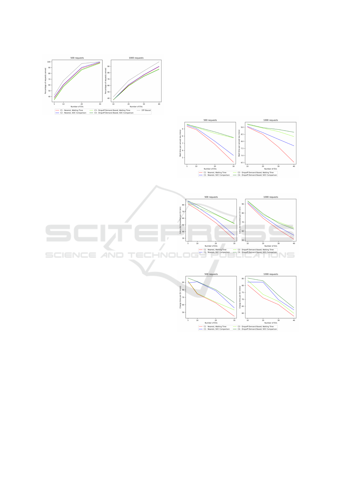
Figure 6: Percentage of requests served.

thus leading to the charging conditions being fulﬁlled

more often, leading to higher charge time. It then de-

creases again because the number of EVs becomes

a more dominant factor compared to the increased

charging time. Also, with more requests, the charg-

ing time increases, as with more load on the system,

each EV serves more requests and loses charge faster,

hence needing to charge more frequently. Another

important observation is that the time spent charg-

ing is higher for algorithms with the SOC comparison

based charging policy. With a higher number of EVs,

more often than not, EVs have other EVs near them,

and the waiting time in the SOC comparison policy

is lower than that in the waiting time policy. So, the

conditions to decide whether to go for charging be-

come less strict in the SOC comparison based policy,

leading to a higher time spent charging by the EVs.

5.3 Scenario 2 - Sampling Based on Trip

Distance

In this case, we sample the requests such that 1/3

the requests have their trip distance (distance between

pickup and dropoff) less than 5 km, another 1/3

the requests have their trip distance between 5 and 10

km, and the remaining 1/3

of the requests have their

trip distance greater than 10 km. Thus the trip dis-

tances are more widely distributed, and also allows

for evaluating the performance when there are more

number of longer trips.

Fig. 6 shows the variation in the percentage of

requests served with the number of EVs. As ex-

pected, the percentage of requests served increases

with an increase in the number of EVs for all the al-

gorithms. The algorithms with the SOC comparison

based charging policy perform slightly better, as in

this case there are more trips with longer distances,

causing them to run out of charge and go for charging

more often. This makes them better prepared for ac-

cepting future requests with long trip distances. For

both 500 and 1000 requests, the best algorithm falls

short of the STF bound by 3-7% only depending on

the number of EVs, showing that the proposed algo-

rithms perform quite well.

Fig. 7, Fig. 8, and Fig. 9 show the variation in

average waiting time per served request, average ex-

tra distance travelled per EV, and average time spent

charging per EV respectively with the number of EVs.

The trends observed here are similar to that of the pre-

vious scenario, for similar reasons as explained ear-

lier.

Figure 7: Waiting time per served request.

Figure 8: Extra distance travelled per EV.

Figure 9: Time spent charging per EV.

5.4 Scenario 3 - Sampling Based on

Pickup Location

In this scenario, we choose a 6 km

area at the centre

of Manhattan, and sample requests such that 70% of

requests have their pickup location inside this desig-

nated area, and the rest 30% have their pickups out-

side this designated area. Often, in the real world, it

happens that for particular times of a day, there is one

area where trafﬁc is concentrated (for example, the

VEHITS 2025 - 11th International Conference on Vehicle Technology and Intelligent Transport Systems

downtown area of a city), and most people request

rides starting from that area. The request sampling

attempts to model this scenario where demand is con-

centrated more in certain areas.

For this scenario, we also perform additional sim-

ulations with the optimization of routing idle EVs en-

abled. However, due to space constraint, we report

results with the optimization enabled only for the best

performing strategy (C4 - Dropoff Demand Based and

SOC Comparison).

Figure 10: Percentage of requests served.

Fig. 10 shows the variation in the percentage of

requests served with the number of EVs. It can be

seen that in this case, C4 performs the best, followed

by C2, C3, and C1 in that order. We also observe that

C4, with the optimization of routing idle EVs to ar-

eas of high demand, gives a 2-3% boost, compared

to C4 without it. This is expected as the demand is

mostly concentrated in one region in this case, and

hence routing EVs back to the area of the city where

there is higher demand helps in serving more requests.

It is seen that the strategies with the demand based

EV assignment perform better than their nearest EV

counterparts, because there is a very distinct demand

pattern in the dataset in this case. Also, the SOC com-

parison based charging policy performs better as com-

pared to the waiting time based policy as more of-

ten than not, after dropping off a passenger, the EV

will not get another request near that dropoff loca-

tion, because the pickups are mostly concentrated in

one area. So, they will need to travel some extra dis-

tance to go back to the location with more requests to

serve the next request. Since with the SOC compar-

ison based policy, EVs go for charging more often,

fewer requests are rejected because of the EVs hav-

ing insufﬁcient SOC to reach a pickup location that is

far, thus leading to more requests being served. With

500 and 1000 requests, the best algorithm falls short

of the STF bound by 11-14% and 5-11% respectively,

depending on the number of EVs. This again shows

that the proposed algorithms perform quite well in

this scenario also.

Figure 11: Waiting time per served request.

Fig. 11 shows the variation in the waiting time per

served request with the number of EVs. It is again ob-

served that the waiting time decreases rapidly with an

increase in the number of EVs. Also, comparing be-

tween C4 with and without the optimization enabled,

we see that the average waiting time for served re-

quests decreases on routing the idle EVs. Routing idle

EVs to areas with high demand allows requests to ﬁnd

an EV both fast and close to the pickup location, thus

leading to a reduction in the waiting time.

Figure 12: Extra distance travelled per EV.

Fig. 12 shows the variation in the extra distance

travelled per EV with the number of EVs. Similar

to the previous two scenarios, the extra distance trav-

elled by EVs is higher for the algorithms with the de-

mand based EV assignment scheme, compared to the

nearest EV assignment scheme, as EVs have to travel

more to reach the pickup location in this case. Also,

the extra distance travelled by EVs increases on rout-

ing the idle EVs. This is understandable as now the

EVs are moving from their location to locations with

higher demand, thus contributing to the extra distance

travelled.

Routing and Charge Planning Strategies for Ridesharing EV Fleets

Figure 13: Time spent charging per EV.

Fig. 13 shows the variation in the time spent

charging per EV with the number of EVs. Again, it

can be seen that the average charging time per EV

decreases with an increase in the number of EVs as

expected. Also, time spent charging is higher when

we route the idle EVs because now they have to travel

more, leading to them running out of charge faster and

more frequently, thus leading to more frequent charg-

ing.

6 CONCLUSION

In this paper, we have addressed the problem of man-

agement of an EV ﬂeet for ridesharing to satisfy pas-

senger requests. We presented a set of four algorithms

for the problem and presented detailed simulation re-

sults on a real world dataset to show that the algo-

rithms perform well. The work can be further ex-

tended by considering other objective functions such

as operator proﬁt, passenger’s ride cost etc., and the

use of a set of mobile charging stations owned by the

ﬂeet operator for EV charging to reduce operator cost.

REFERENCES

Chen, T., Zhang, B., Pourbabak, H., Kavousi-Fard, A.,

and Su, W. (2018). Optimal routing and charging of

an electric vehicle ﬂeet for high-efﬁciency dynamic

transit systems. IEEE Transactions on Smart Grid,

9(4):3563–3572.

Chen, T. D., Kockelman, K. M., and Hanna, J. P. (2016).

Operations of a shared, autonomous, electric vehicle

ﬂeet: Implications of vehicle & charging infrastruc-

ture decisions. Transportation Research Part A: Pol-

icy and Practice, 94:243–254.

Donovan, B. and Work, D. (2016). New

york city taxi trip data (2010-2013).

https://doi.org/10.13012/J8PN93H8.

Guo, G. and Xu, Y. (2022). A deep reinforcement learn-

ing approach to ride-sharing vehicle dispatching in au-

tonomous mobility-on-demand systems. IEEE Intel-

ligent Transportation Systems Magazine, 14(1):128–

140.

Guo, Z., Hao, M., Yu, B., and Yao, B. (2021). Robust

minimum ﬂeet problem for autonomous and human-

driven vehicles in on-demand ride services consider-

ing mixed operation zones. Transportation Research

Part C: Emerging Technologies, 132:103390.

Hua, Y., Zhao, D., Wang, X., and Li, X. (2019). Joint in-

frastructure planning and ﬂeet management for one-

way electric car sharing under time-varying uncertain

demand. Transportation Research Part B: Method-

ological, 128:185–206.

all, C., Ceder, A., Ekstr

om, J., and Quttineh, N.-H. (2018).

Adjustments of public transit operations planning pro-

cess for the use of electric buses. Journal of Intelligent

Transportation Systems, 23:1–15.

Kullman, N. D., Cousineau, M., Goodson, J. C., and Men-

doza, J. E. (2022). Dynamic ride-hailing with electric

vehicles. Transportation Science, 56(3):775–794.

Lin, B., Ghaddar, B., and Nathwani, J. (2021). Electric

vehicle routing with charging/discharging under time-

variant electricity prices. Transportation Research

Part C: Emerging Technologies, 130:103285.

Lin, K., Zhao, R., Xu, Z., and Zhou, J. (2018). Efﬁcient

large-scale ﬂeet management via multi-agent deep re-

inforcement learning. In 24th ACM SIGKDD Interna-

tional Conference on Knowledge Discovery & Data

Mining, page 1774–1783.

Lu, J.-L., Yeh, M.-Y., Hsu, Y.-C., Yang, S.-N., Gan, C.-H.,

and Chen, M.-S. (2012). Operating electric taxi ﬂeets:

A new dispatching strategy with charging plans. In

2012 IEEE International Electric Vehicle Conference,

pages 1–8.

Ma, T.-Y. and Fang, Y. (2022). Survey of charging man-

agement and infrastructure planning for electriﬁed

demand-responsive transport systems: Methodologies

and recent developments. European Transport Re-

search Review, 14.

Ma, T.-Y. and Xie, S. (2021). Optimal fast charging sta-

tion locations for electric ridesharing with vehicle-

charging station assignment. Transportation Research

Part D: Transport and Environment, 90:102682.

Mor, A. and Speranza, M. (2020). Vehicle routing problems

over time: a survey. 4OR, 18.

Nissan (2023). Nissan leaf features.

https://www.nissanusa.com/vehicles/electric-

cars/leaf/features.html.

Schiffer, M. and Walther, G. (2017). The electric loca-

tion routing problem with time windows and partial

recharging. European Journal of Operational Re-

search, 260(3):995–1013.

Schiffer, M. and Walther, G. (2018). Strategic planning

of electric logistics ﬂeet networks: A robust location-

routing approach. Omega, 80:31–42.

Shehadeh, K. S., Wang, H., and Zhang, P. (2021). Fleet

sizing and allocation for on-demand last-mile trans-

portation systems. Transportation Research Part C:

Emerging Technologies, 132:103387.

Shi, J., Gao, Y., Wang, W., Yu, N., and Ioannou, P. A.

(2020). Operating electric vehicle ﬂeet for ride-

VEHITS 2025 - 11th International Conference on Vehicle Technology and Intelligent Transport Systems

hailing services with reinforcement learning. IEEE

Transactions on Intelligent Transportation Systems,

21(11):4822–4834.

Stumpe, M., R

oßler, D., Schryen, G., and Kliewer, N.

(2021). Study on sensitivity of electric bus systems

under simultaneous optimization of charging infras-

tructure and vehicle schedules. EURO Journal on

Transportation and Logistics, 10:100049.

Wang, Y., Bi, J., Guan, W., and Zhao, X. (2018). Opti-

mising route choices for the travelling and charging of

battery electric vehicles by considering multiple ob-

jectives. Transportation Research Part D: Transport

and Environment, 64:246–261.

Wu, X., Feng, Q., Bai, C., Lai, C. S., Jia, Y., and Lai, L. L.

(2021). A novel fast-charging stations locational plan-

ning model for electric bus transit system. Energy,

224:120106.

Yu, G., Liu, A., Zhang, J., and Sun, H. (2021). Opti-

mal operations planning of electric autonomous ve-

hicles via asynchronous learning in ride-hailing sys-

tems. Omega, 103:102448.

Zalesak, M. and Samaranayake, S. (2021). Real time op-

eration of high-capacity electric vehicle ridesharing

ﬂeets. Transportation Research Part C: Emerging

Technologies, 133:103413.

Zhang, H., Sheppard, C. J. R., Lipman, T. E., and Moura,

S. J. (2020). Joint ﬂeet sizing and charging sys-

tem planning for autonomous electric vehicles. IEEE

Transactions on Intelligent Transportation Systems,

21(11):4725–4738.

Routing and Charge Planning Strategies for Ridesharing EV Fleets