Multi-Perspective Analyses of Spatio-Temporal Data About Well-Being
Yunji Zhang
1 a
, Franck Ravat
2 b
and S
´
ebastien Laborie
1 c
and Philippe Roose
1 d
1
Universite de Pau et des Pays de l’Adour, E2S UPPA, LIUPPA, Anglet, France
2
Institut de Recherche en Informatique de Toulouse - Universit
´
e Toulouse Capitole, 31000, Toulouse, France
Keywords:
Data Analysis, On-Read Schema, Spatio-Temporal Data, Multi-Perspective Analysis, Well-Being.
Abstract:
The concept of ”Well-being” within local territories is increasingly recognized as a critical issue by local
decision-makers. In the face of demographic shifting and population ageing, decision-makers need to an-
ticipate demographic changes, plan land use, and shift land use promptly. They need a broader perspective
that integrates various dimensions of the living environment for their territories. Therefore, it requires a sys-
tem that can integrate different datasets and perspectives on various dimensions of ”Well-being”, including
demographics, population distribution, land utilisation, transport, infrastructure development, social and busi-
ness services, etc. It can perform comprehensive multi-perspective analyses based on integrated perspectives.
However, the existing work on this topic mainly focuses on a single-perspective analysis, such as focusing
exclusively on education. In order to fill this gap, this article aims to propose: (i) a mind map outlining the
dimensions related to ”Well-being” and the associated data required for analyses; (ii) an on-read schema mod-
elling framework for the storage, the cross-integration and the promoting accessibility of the multi-perspective
data; and (iii) a modelling concept for multi-perspective analysis data to represent the various dimensions re-
lating to ”Well-being”.
1 INTRODUCTION
The world population is projected to increase by 2
billion, from 7.7 billion today to 9.7 billion in 2050,
and to peak at nearly 11 billion by the end of the cen-
tury. This phenomenon is affecting economic stabil-
ity, healthcare systems, and social dynamics on an un-
precedented scale. To face this demographic shift, a
new goal for worldwide Well-being promotes healthy
lifestyles with a modern and efficient living environ-
ment for all ages
1
. Addressing the challenges and
taking advantage of the opportunities presented by the
new goal of achieving global well-being is not just a
policy issue, but an imperative to ensure that the world
achieves sustainable and inclusive development. Lo-
cal decision-makers want to comprehensively under-
stand the area’s living environment to improve the
facilities and services available to support a ”Well-
being” society. Therefore, decision-makers need to
a
https://orcid.org/0009-0004-7411-7647
b
https://orcid.org/0000-0003-4820-841X
c
https://orcid.org/0000-0002-9254-8027
d
https://orcid.org/0000-0002-2227-3283
1
https://www.un.org/ga/search/view doc.asp?symbol=
A/RES/70/1&Lang=E
comprehensively analyse the local living environment
from multiple perspectives to make recommendations
for improving the local living environment.
Most of the current research about ”Well-being”
focuses mainly on how a single perspective affects
”Well-being”, such as how education affects well-
being (Arthur J. Reynolds, 2011), what is the rela-
tionship between transport and well-being (Reardon
and Abdallah, 2013), how can urban planning im-
prove well-being (Patel, 2011), what kind of med-
ical system can ensure Well-being (Anne De Biasi
and Auerbach, 2020). Decision-makers lack a multi-
perspective analysis which provides a whole picture
of the local living environment.
We identified 9 dimensions of Well-being. Af-
ter defining the multi-thematic analysis structure, we
found that our study is facing two major challenges
after reading related studies and searching for open
data related to each dimension.
Challenge 1: Multi-Perspective Analyses. Building
a multi-perspective analysis involves more than just
collecting and analysing data from a single topic. It
requires integrating data from different themes and
identifying relationships between them, for exam-
ple, changes in environmental conditions may affect
80
Zhang, Y., Ravat, F., Laborie, S. and Roose, P.
Multi-Perspective Analyses of Spatio-Temporal Data About Well-Being.
DOI: 10.5220/0013282800003928
Paper published under CC license (CC BY-NC-ND 4.0)
In Proceedings of the 20th International Conference on Evaluation of Novel Approaches to Software Engineering (ENASE 2025), pages 80-91
ISBN: 978-989-758-742-9; ISSN: 2184-4895
Proceedings Copyright © 2025 by SCITEPRESS – Science and Technology Publications, Lda.

health outcomes.
Challenge 2: Heterogeneous Datasets. Datasets re-
lating to different dimensions are heterogeneous with
different minimum granularity and scopes. It causes
an inevitable problem when we want to compare or
integrate one dataset with another.
Therefore, our research needs to answer the fol-
lowing 2 questions:
• How to build a system that can provide multi-
perspective analyses?
• How to build a system that integrates heteroge-
neous datasets with different structures, scopes
and granularity?
In order to achieve this goal, we decided to build
an on-read schema modelling framework for stor-
age, cross-integration, and the accessibility multi-
dimension data analysis. This model allows us to
store all kinds of datasets relating to ”Well-being”
with notions of time and space. The integration will
only be done with the user’s demand, which could
greatly reduce the time of heterogeneous data integra-
tion at the beginning of model construction.
In this paper, after introducing the background and
related work, we present the concept of the on-read
schema for raw data and the concept of the analytic
data model. Then, we explore possible future di-
rections of a model for multi-perspective analyses to
show how a territory changes over time on various di-
mensions relating to ”Well-being”.
2 BACKGROUND
The concept of ”Well-being” is a comprehensive con-
cept that includes physical health, mental health, so-
cial relationships, economic well-being, emotional
fulfilment, etc. In the 21st century, it has been stud-
ied extensively by psychologists and social scientists,
particularly in the field of positive psychology(Ryff
and Singer, 2008). ”Well-being” has become one of
the most important individual and societal well-being
indicators.
Given this context, the concept of ”Well-being”
is increasingly recognized as a critical issue by lo-
cal decision-makers. To identify the dimensions as
the base of our research, we built a multidimensional
analysis framework of ”Well-being”.
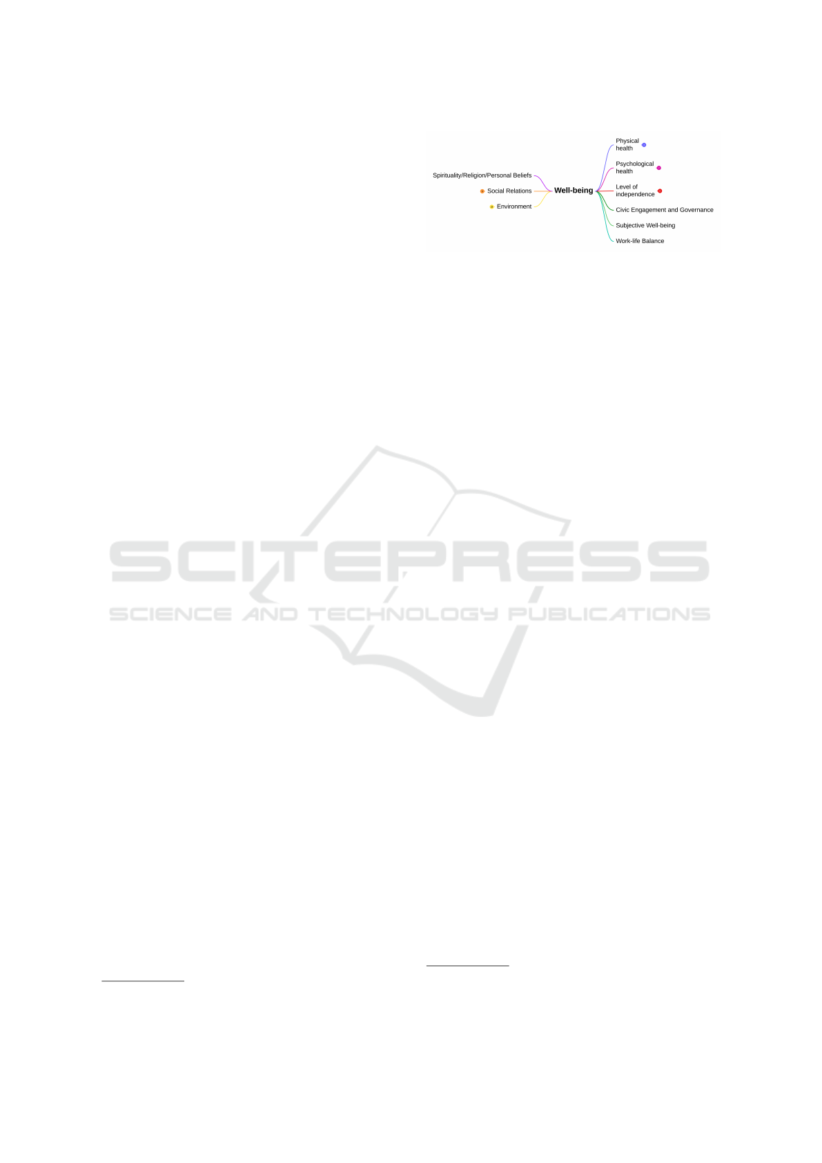
Through research on measures proposed by inter-
national organisations (OECD, 2011; WHO, 2023),
we proposed an analysis framework of well-being that
includes 9 dimensions (Figure 1). For each dimen-
sion, we identified sub-analysis branches
2
. Based on
2
Entire framework: http://bit.ly/3PIXEol
Figure 1: Main dimensions of Well-being.
this analysis framework, we search and identify rele-
vant accessible data for each analysis theme (dimen-
sion) and its sub-themes (sub-branches).
There are two main types of data sources:
• Internal Data Sources: they provide data about
the target territory.Local councils and other local
companies usually provide this part of data. It is
usually high-quality, with fewer null values and
clear descriptions. However, due to the lack of
data from other departments and regions, we are
unable to make a comparative analysis.
• External Data Sources: they are usually Open
Data, providing a wider range of areas or a differ-
ent region. This part of data may have a lower
quality and more null values. It could also be
more aggregate. We use this data to compare with
internal data or to give a more general view.
As mentioned earlier, the diversity of data sources
leads to differences in the structure, type, scopes and
granularity of the datasets.
In terms of structure and type, current data range
from structured, such as Excel and CSV (e.g., Direc-
tory of social landlords’ rental accommodation
3
), to
semi-structured, such as JSON, GEOJSON, Shapefile
and XML (e.g., Landes - Emergency call centres
4
).
In terms of granularity, the minimum spatial granu-
larity may be geographic point and the maximum may
be country; the minimum temporal granularity may
be date and the maximum may be year.
In terms of scope, the current database covers a spa-
tial range of up to all countries in the world, and down
to one or a few cities; and a temporal range of up to
1900 to the present, and down to one year.
Therefore, we need to build a system that can
integrate these heterogeneous datasets for multi-
perspective analyses.
3
https://bit.ly/40lfm6k
4
https://bit.ly/4jfBLe1
Multi-Perspective Analyses of Spatio-Temporal Data About Well-Being
81

3 RELATED WORK
3.1 Well-Being
Various disciplines (e.g., medicine, psychology, soci-
ology, economics) include research on ”Well-being”.
They mainly focuses on how a single perspective af-
fects the situation of ”Well-being” statistically. From
the education perspective, researchers reported indi-
cators showing that early education can positively im-
pact future well-being (Arthur J. Reynolds, 2011).
From the urbanise perspective, researchers clarified
the inter-relationships between various fundamental
parameters in the design of an urban layout to im-
prove our understanding of urban layouts and the
complicated trade-offs between desirable features and
another (Patel, 2011). From the transport perspective,
researchers built a dynamic model that provides the
most comprehensive and integrated discussion of the
current well-being literature from a transport perspec-
tive (Reardon and Abdallah, 2013). From the medi-
cal perspective, researchers outlined roles that public
health could fulfil, in collaboration with ageing ser-
vices, to address the challenges and opportunities of
an ageing society (Patel, 2011).
However, little research focuses on a multi-
perspective analysis of ”Well-being” from the view of
data analytics. No analysis system adapts well to var-
ious ”Well-being” dimensions or provides decision-
makers with readable, visual reports on current and
future trends. Our research aims to address this by
integrating different datasets related to dimensions of
”Well-being”, such as demographics, population dis-
tribution, land use, transport, infrastructure, and so-
cial and business services. This integration will en-
able comprehensive analyses from multiple perspec-
tives.
3.2 Integration of Spatio-Temporal
Data
Well-being data are generally characterized as spatio-
temporal. The systems analyzing these types of data
are organized into three main modules (Md Mah-
bub Alam and Bifet, 2022): (1) data storage, which
includes both spatial relational database management
system and NoSQL databases (Felix Gessert and Rit-
ter, 2017); (2) data processing, which encompasses
big data infrastructure sorted by architecture types
(e.g., Hadoop
5
, Spark
6
, NoSQL (Ali Davoudian and
Liu, 2018)) and data processing systems (e.g., spatial
5
https://hadoop.apache.org/
6
http://spark.apache.org/
(Ahmed Eldawy and Mokbel, 2017), spatio-temporal
(Nidzwetzki and G
¨
uting, 2019), trajectory (Xin Ding
and Bao, 2018)); and (3) data programming and
software tools, covering libraries and software like
R, Python (Zhang and Eldawy, 2020), ArcGIS
7
and
QGIS
8
that support processing of spatial and spatio-
temporal data.
Considering the integration of spatio-temporal
data, data from different sources could have distinct
spatial and temporal resolutions, which leads to dif-
ferent spatial and temporal granularity. In terms
of space, new data are usually at a higher resolu-
tion than old data due to technological developments,
e.g., aerial photographs, satellite imagery or other re-
motely sensed data. At the same time, the spatial res-
olution of different data sources may vary, for exam-
ple, highway data are usually specific to geographic
points, while weather-related data are mostly by city.
In terms of time, data such as rivers and lakes, admin-
istrative boundaries, and roads have a relatively low
temporal resolution and can be considered static; data
such as weather is usually updated hourly; and traffic
conditions, for example, may change within seconds
(Le, 2012). The data that will be used for analyses of
”Well-being” include structured data, semi-structured
data and non-structured data. Meanwhile, since we
are in real-world applications, there is a large amount
of spatio-temporal information which is often vague
or ambiguous with low quality due to missing values,
high data redundancy, and untruthfulness (Luyi Bai
and Bai, 2021). Therefore, we can conclude that we
are dealing with standard heterogeneous data (Wang,
2017).
Considering the big data scenario for ”Well-
being” data, data lakes (DL) are considered a use-
ful data storage method. Data lakes emerge as a big
data repository that stores raw data and provides a rich
list of features with the help of metadata descriptions
(Khine and Wang, 2018). Data ingestion is simple as
there is no need for a data schema or ETL (Extract-
transform-load) process design. It is also horizon-
tally and vertically scalable as there is no fixed data
schema. Therefore, Data Lake is a perfect solution
for heterogeneous data with various types and granu-
larity.
7
https://www.arcgis.com/index.html
8
https://www.qgis.org
ENASE 2025 - 20th International Conference on Evaluation of Novel Approaches to Software Engineering
82

4 DATA MODELLING
4.1 Overall Modelling Architecture
Considering the diversity of data sources, we propose
to create an on-read schema in a data lake. As we
introduced in the previous section, our datasets are
heterogeneous with different structures, types, scopes
and granularity. We do not integrate the data right
after the extraction but ingest them in their native for-
mat, and only integrate data according to a specific
requirement.
This approach has three benefits:
No Need for Data Structure and ETL Process De-
sign. If we want to integrate all data right after the
extraction, we need to analyse all user’s requirements
and spend a long time constructing the structure and
ETL process at the beginning of model construction.
Instead of a traditional ETL process, we use the ELT
(Extract-load-transform) process.
Reduce the Integration Time. Due to the large anal-
ysis framework and varied themes, not all datasets are
necessarily used for users’ analysis requirements. To-
gether with the serious heterogeneity of datasets, each
additional dataset that needs to be integrated will in-
crease data integration time. Integrating all datasets
without specific requirements is wasteful.
Get a Horizontally and Vertically Scalable Struc-
ture. We choose to build a data lake with Raw data
zone and Analysis data zone (Ravat and Zhao, 2019).
We first pre-process datasets when we extract data
from internal and external sources to ensure their
quality (e.g., data cleaning and harmonisation of data
formats). Then in the raw data zone (§4.2), we ex-
tract and load datasets and store them in a near-native
format. We automatically extract the file’s metadata:
• Basic information about file: title, source (URL),
update frequency, file type
• Containing information: parameters, complemen-
tary information, measures
• Corresponding theme
• Spatial information: spatial granularity, spatial
scopes, applicable spatial hierarchies
• Temporal information: temporal granularity, tem-
poral scopes, applicable temporal hierarchies
After the user proposes a requirement with
themes, minimum spatio-temporal granularity and
spatio-temporal scopes, we select the appropriate
datasets from the raw data zone. We extract exist-
ing indicators and create new cross-theme indicators
while integrating the datasets with an aggregation-
union measure in the analysis area (§4.3). We record
the metadata of integration and indicators in the gov-
ernance area for repeated requirements and future vi-
sualisation and analysis.
4.2 Raw Data Zone
In the raw data zone, we propose a multi-view data
storage. The data ingestion in the raw data zone
is based on: contained information, theme with cat-
alogue, spatial view with hierarchies and temporal
view with hierarchies. We classify data in datasets
into three types:
Parameters are attributes linking to a particular level
our predefined spatial and temporal hierarchies.
Complementary information is non-computable at-
tributes, can be additional information of parameters.
Measure is computable information that links to one
specific theme and will be considered as indicators in
the analysis data zone.
All the information of datasets related to the file
or the ingestion is stored in the metadata.
4.2.1 Predefined Theme Catalogue and
Spatio-Temporal Hiererachies
Theme Catalogue
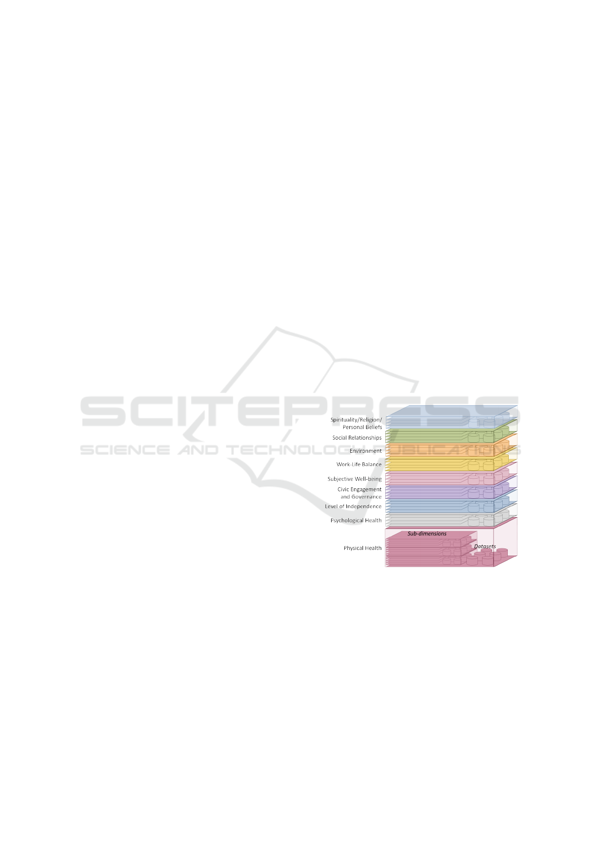
Figure 2: Multi-layer structure.
The theme catalogue is based on the previously men-
tioned analysis framework. Whether internal or exter-
nal, each dataset we extract is affiliated with a partic-
ular analysis theme (dimension at any branch level in
the framework). We consider each theme in the anal-
ysis framework (Figure 1) as a layer and their sub-
themes as their sub-layers. The datasets are stored
in their original format in the corresponding layer ac-
cording to the theme of the information they contain.
Thus, the basic structure of raw data can be seen as
a multi-layer structure differentiated by the dimen-
sion of the analysis framework (Figure 2). Each layer
Multi-Perspective Analyses of Spatio-Temporal Data About Well-Being
83

(theme) has 0 to n subsidiary datasets and 0 to n sub-
layers (sub-themes).
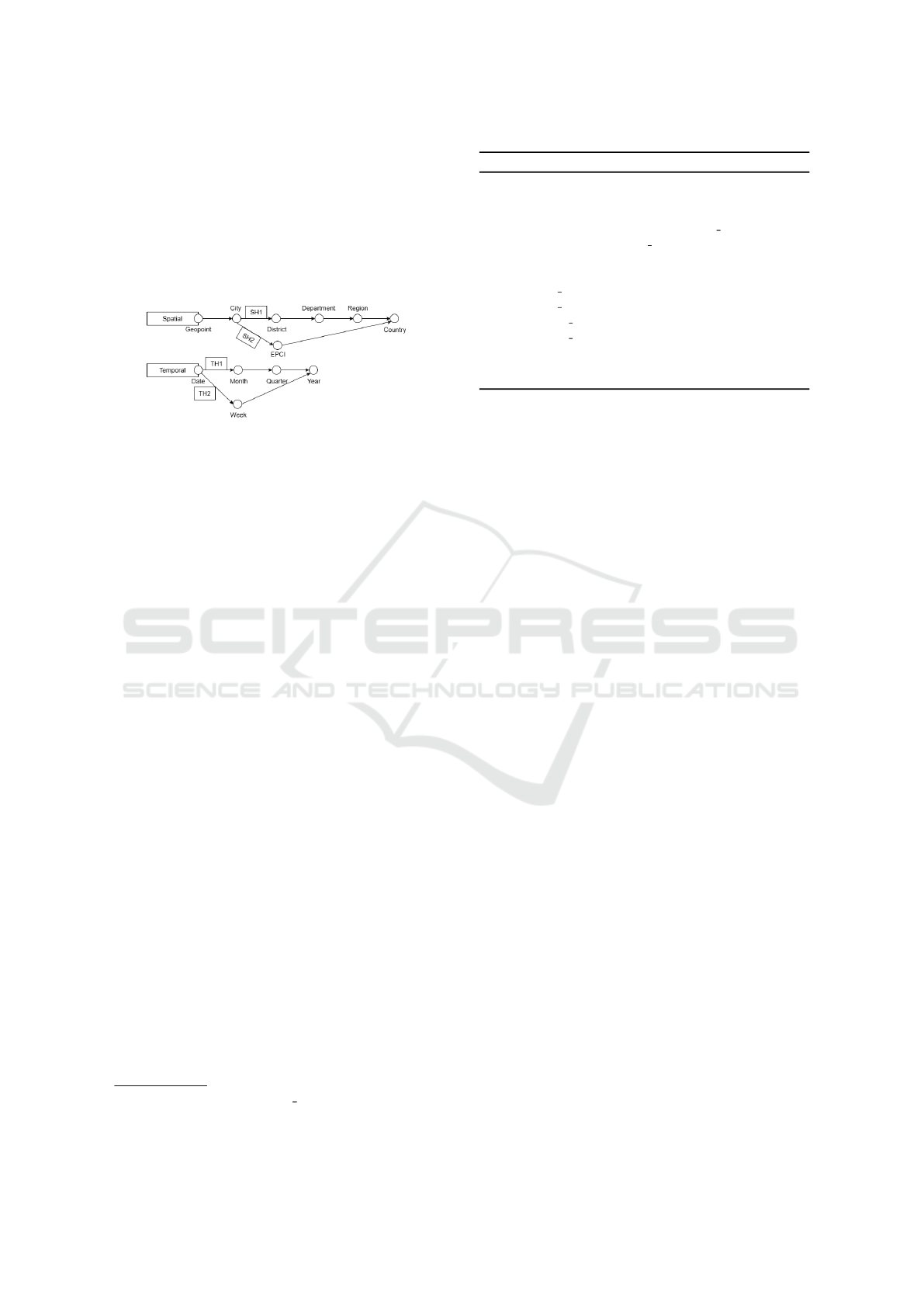
Spatial and Temporal Hierarchies
Meanwhile, according to GADM Dataset of France
9
and Generate Calendar Dataset
10
, we propose two
hierarchies. Each hierarchy classifies the spatial or
temporal concept from the lowest level to the highest
(Figure 3).
Figure 3: Predefined Hierarchies.
4.2.2 Dataset Ingestion
In order to ingest datasets, we extract information
from four points of view:
1. Information Contained: we identify the parame-
ters, complementary information and measures of
a dataset.
2. Spatial Information: according to its spatial pa-
rameters, we link the dataset to predefined spatial
hierarchies by its spatial minimum granularity and
identify its spatial scope.
3. Temporal Information: according to its tempo-
ral parameters, we link the dataset to predefined
temporal hierarchies by its spatial minimum gran-
ularity and identify its temporal scope.
4. Theme: according to the complementary infor-
mation and measures of a dataset, we locate
the dataset into the tree structure of the analysis
framework.
We record this information of each dataset in
metadata. The metadata structure is shown in Figure
4. The classes in red (Theme and Hierarchy) are pre-
defined and the other classes are generated based on
each ingested dataset. The program of data ingestion
is shown in Algorithm 1. The formal expression of
the above concept is as follows:
• In one theme layer, there are 0 to n sub-layers and
0 to m related datasets:
T
i
= {{T
i,1
, T
i,2
, ..., T
i,n
}, {D
1
, D
2
, ..., D
m
}} (1)
• We record the following information of each
dataset:
9
https://gadm.org/download country.html
10
https://github.com/Marto32/gencal
Algorithm 1: Raw Dataset Ingestion Algorithm.
Input: Dataset DS
Output: Metadata MD
Identify
DS.identi f ication, DS.ingestion, DS.data content, DS.theme
Classify columns in DS.data content into Spatial
Parameters (SP), Temporal Parameters (TP),
Complementary Information (CI), Measures (M)
DS.spatial granularity ← max(SP.spatialLevel);
DS.spatial scope ← min(SP.spatialLevel);
DS.temporal granularity ← max(T P.temporalLevel);
DS.temporal scope ← min(T P.temporalLevel);
Build metadata MD
Copy DS to thematic catalogue DS.theme
return MD
D
i
= {{{SP
1
, SP
2
, ..., SP
n
}, {T P
1
, T P
2
, ..., T P
m
}},
{CI
1
[T
i, j
], CI
2
[T
i,k
], ..., CI
p
}, {M
1
[T
i, j
], M
2
[T
i,k
],
..., M
q
[T
i,l
]}, SG, SS, T G, T S,
{{SH
1
, SH
2
, ...}, {T H
1
, T H
2
, ...}}, T [i]}
(2)
- T: Theme
- D: Dataset
- SP: Spatial parameter
- TP: Temporal parameter
- CI: Complementary information
- M: Measure
- SG: Minimum spatial granularity
- TG: Minimum temporal granularity
- SS: Spatial scope
- TS: Temporal scope
- SH: Spatial hierarchy
- TH: Temporal hierarchy
The final structure of the raw data zone is shown in
Figure 5. The metadata of all raw data zone datasets
is stored in the governance zone of the data lake and
it gets updated within the ingestion of new datasets.
4.2.3 Example
Taking the CSV file National Register of Condomini-
ums in theme Domestic environment as an example:
This dataset contains the following parameters:
spatialPs = {EPCI, Commune, [long, lat], Code Officiel
D
´
epartement, Code Officiel R
´
egion, ...}
temporalPs = {Date du r
`
eglement de copropri
´
et
´
e}
Therefore, we can identify the minimum spatial
and temporal granularity:
spatialGranularityMin = Geographic point
temporalGranularityMin = Date
From the parameters, we can also get its spatial
and temporal scope:
scopeSpatial = {Region: [’11’, ’3’, ...]}
scopeTemp = {startPoint = ”1900-01-01”, endPoint =
”2021-12-31”}
ENASE 2025 - 20th International Conference on Evaluation of Novel Approaches to Software Engineering
84

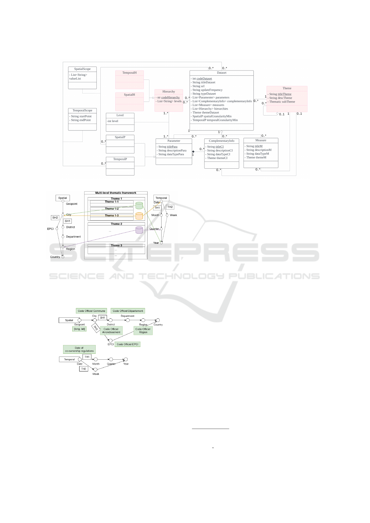
Figure 4: Metadata of raw data.
Figure 5: Data Storage in Raw Data Zone.
We choose the corresponding predefined spatial
and temporal hierarchies according to the granularity
and scope. The parameter in our example correspond
to the predefined hierarchies as Figure 6.
Figure 6: How Parameters Correspond Hierarchies.
As we can see in Formal Expression 2, the theme
of a dataset is the least common theme of its comple-
mentary information and measures.
Complementary information can correspond to a
parameter, such as Commune Official Name corre-
sponds to the parameter Commune Official Code.
Measures are statistical attributes, such as Number
of Parking Lots. Each measure must be related to a
theme. For example, Number of Parking Lots links to
the theme Available equipment. In the metadata file,
we record it in the following form
11
:
Dataset = {
codeDataset = 1
titleDataset = National Register of Condominiums
url = https://bit.ly/ 3Y8SOoq
updateFrequency = Quarterly
typeDataset = csv
themeDataset = Domestic Environment
parameters = {{[long, lat], ...},{Date of co-
ownership regulations}}
complementaryInfo = {Commune Official
Name, Construction
period [Building con-
struction quality],
...}
measures = {Number of Parking Lots [Avail-
able equipment], ...}
hierarchies = {SH1, SH2, TH1, TH2}
spatialGranularityMin = Geopoint
temporalGranularityMin = Date
spatioScope = {Country:{France}}
temporalScope = {startPoint
¯
1900-01-01,
endPoint
¯
2021-12-31}
}
4.3 Analysis Data Zone
Datasets are retained in their native format in the raw
data zone until a user’s requirement appears. We start
the analysis when a user selects the themes of analy-
sis, the spatial and temporal granularity of the analysis
and the spatial and temporal scope from our analysis
11
Metadata of the dataset National Register
of Condominiums: https://github.com/Yunji5264/
Example Complete-Metadata
Multi-Perspective Analyses of Spatio-Temporal Data About Well-Being
85

framework and predefined hierarchies as his/her re-
quirement. For example, a user selects:
• Themes: Domestic Environment, Pollution
• Spatial Granularity: Geopoint
• Spatial Scope: Country: France
• Temporal Granularity: Date
• Temporal Scope: startPoint = 2021-01-01, end-
Point = 2024-12-31
4.3.1 Preparation of Corresponding Dataset
We filter the corresponding data and its datasets from
the raw data zone based on an user requirement. The
datasets meet the following three conditions:
1. They are contained under the folder of the selected
themes or any of their contents (complementary
information or measures) belongs to these themes.
2. The corresponding spatio-temporal scope of the
dataset lies within the selected scope.
3. Their corresponding spatio-temporal granularity
is finer than or equal to the selected granularity.
After filtering, we determine whether the raw data
zone contains sufficient data to answer the require-
ment. If not, we propose possible modifications in
requirements to users:
1. Select a more general minimum granularity (anal-
ysis parameters)
2. Select wider scopes
3. Select of more general themes
Algorithm 2: Granularity Adjustment Proposal.
Input: Required spatial granularity RSG,
Required temporal granularity RT G,
Predefined spatial hierarchies SH,
Predefined temporal hierarchies T H
Output: Alternative granularity options ST G
Initialize ST G as an empty list;
foreach Spatial granularity sg in levels equal to or
more general than RSG from SH do
foreach Temporal granularity tg in levels
equal to or more general than RT G from T H
do
if not(sg = RSG and tg = RT G) then
Add [sg, tg] into ST G;
end
end
end
return ST G;
In our example, supposing the finest granularity
of all datasets in both themes (Domestic Environment
and Pollution) is not Geopoint - Date. No data in the
Table 1: Protential granularity.
Spatial granularity Temporal granularity
Geopoint Month
Geopoint Year
City Date
City Month
City Year
Department Date
Department Month
Department Year
raw data zone can meet the user’s requirement. There-
fore, we propose a possible modification by selecting
more general granularity shown in Algorithm 2. In
our example, we offer to the user Table 1 as the pos-
sible alternate granularity.
Suppose the user finally selects City - Year from
Table 1 as the granularity of his/her requirement. The
modified requirement is shown below :
• Themes: Domestic Environment, Pollution
• Spatial Granularity: City
• Spatial Scope: Country: France
• Temporal Granularity: Year
• Temporal Scope: startPoint = 2021-01-01, end-
Point = 2024-12-31
Algorithm 3: Data Integration.
Input: Requirements R, datasets D,
spatial/temporal hierarchies SH, T H
Output: Integrated system IS with indicators
Initialize IS as empty;
foreach granularity pair (SG, T G) from finest to
RSG, RT G do
foreach dataset d ∈ D at SG-T G do
Add indicators from d to IS;
Construct and add cross-theme
indicators;
foreach d
′
in D with higher granularities
do
Aggregate d, d
′
;
Construct and add indicators;
end
end
end
return IS
We then confirm that the existing data meets the
new requirement.
4.3.2 Datasets Integration and Indicators
Construction
After confirming that the existing data meets the re-
quirement in terms of themes, scope and granularity,
ENASE 2025 - 20th International Conference on Evaluation of Novel Approaches to Software Engineering
86

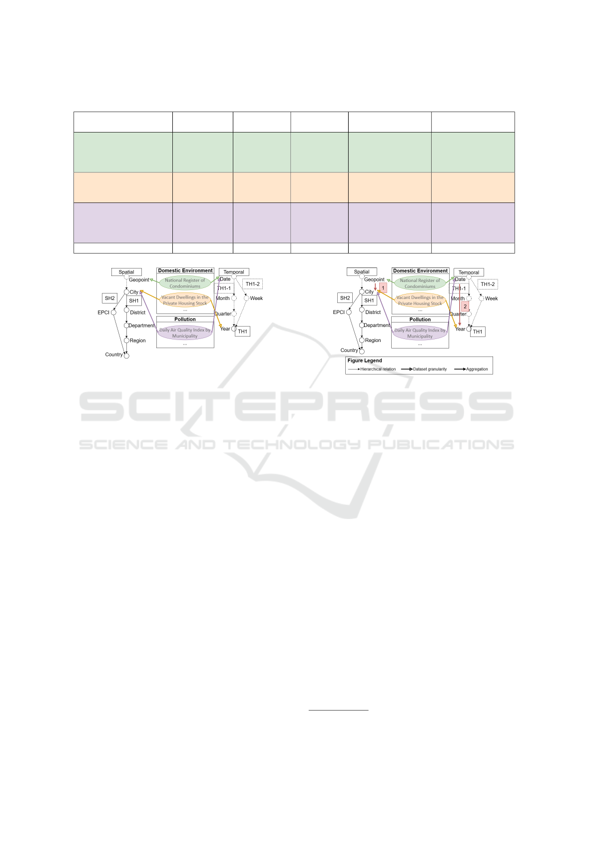
Table 2: Example - Datasets corresponding to requirement.
Source Theme
Spatial
granularity
Temporal
granularity
Spatial scope Temporal scope
National Register of
Condominiums
Domestic
environment
Geopoint Date
Department: ’11’,
’3’, ’32’, ...
startPoint =
’1900-01-01’,
endPoint =
’2024-06-30’
Vacant Dwellings in the
Private Housing Stock
Domestic
environment
City Year
Region:
’Grand-Est’,
’Occitanie’, ...
startPoint = ’2019’,
endPoint = ’2021’
Daily Air Quality Index
by Municipality
Pollution City Date Country: ’France’
startPoint =
’2023-06-11’,
endPoint =
’2024-11-12’
... ... ... ... ... ...
Figure 7: Example - Data Storage in Raw Data Zone.
we get the datasets from the raw data zone. In our ex-
ample, we select the datasets in Table 2 according to
the data storage shown in Figure 7.
The traditional spatio-temporal data integration
approach usually involves finding the minimum con-
ventional granularity between datasets. Assuming
we have a dataset with Date as minimum temporal
granularity and another dataset with Month as min-
imum temporal granularity, the dataset with a mini-
mum temporal granularity of date will be aggregated
to the month level at the time of integration. While
this approach makes it easy to match datasets, spe-
cific information about the dataset with finer gran-
ularity is lost. This may undermine the possibility
of providing cross-topic metrics, as the relationships
(statistical or semantic) present in the dataset may be
at a finer level of granularity. Therefore, we propose
a level-by-level aggregation union approach that can
successfully match datasets without causing relation-
ship loss.
Thanks to the metadata for the raw data zone, we
can easily find the existing possible indicators from
each dataset: all the complementary information link-
ing to a specific theme and the measures. With the
requirement, we can find the part of hierarchies re-
quired. We go through each spatio-temporal granu-
larity to integrate the datasets. The process is shown
in Algorithm 3.
Figure 8 shows the required hierarchies in our ex-
Figure 8: Example - Data with Required Hierarchies.
ample. The solid line indicates the hierarchic levels
involved in the user’s requirement, and the dotted line
indicates the part that exists in the predefined hierar-
chies but is not demanded by the users. We start the
integration from the green dataset with the finest gran-
ularity Geopoint-Date. After recording the original
indicators in this dataset, we firstly aggregate it to the
City-Date level to match with the purple dataset (Red
flash 1 in Figure 8). We construct cross-theme indi-
cators if there is any statistic or semantic relation be-
tween these two datasets. Then we aggregate the two
datasets and the cross-theme indicators we construct
to the City-Year level to match with the orange dataset
(Red flash 2 in Figure 8). We repeat the same process
to construct cross-them indicators. Since City-Year
is the spatio-temporal granularity of the requirement
and we have matched all the selected datasets, the in-
tegration is down. We proposed a meta-model for the
analysis data zone
12
. If any indicator exists in the
raw data zone, we record its source dataset. If it is a
cross-theme indicator, we record its underlying indi-
cators (those from which statistical or semantic rela-
tionships are found). We also record the possible ag-
gregation methods for each indicator. These methods
will be demonstrated to users in the future analytical
tools we develop.
12
https://bit.ly/4ahpW31
Multi-Perspective Analyses of Spatio-Temporal Data About Well-Being
87

The formal expression of the above concept is as
follows:
• For each requirement, there are 1 to n themes,
spatio-temporal granularity and spatio-temporal
scope:
R
i
= {{T
1
, T
2
, ..., T
n
}, SG, T G, SS, T S}
(3)
- R: Requirement
- T: Theme
- SG: Minimum spatial granularity
- TG: Minimum temporal granularity
- SS: Spatial scope
- TS: Temporal scope
• According to the requirement, we select existing
datasets:
R
i
{{T
1
, T
2
, ..., T
n
}, SG, T G, SS, T S}
⇒ {D
1
{{CI
1,1
, CI
1,2
, ..., CI
1, p
},
{M
1,1
, M
1,2
, ..., M
1,q
}},
D
2
{{CI
2,1
, CI
2,2
, ..., CI
2, p
},
{M
2,1
, M
2,2
, ..., M
2,q
}},
..., D
n
{{CI
n,1
, CI
n,2
, ..., CI
n, p
},
{M
n,1
, M
n,2
, ..., M
n,q
}}}
(4)
- D: Dataset
- CI: Complementary information
- M: Measure
• Each indicator has minimum spatial and tempo-
ral granularity, spatio-temporal scopes and themes
and possible aggregation methods. We record the
source dataset for existing indicators and the un-
derlying indicators for cross-theme indicators:
EI
i
= {{T
1
, T
2
, ..., T
n
}, SG, T G, SS, T S,
D, {PA
1
, ..., PA
k
}}
(5)
CT I
i
= {{T
1
, T
2
, ..., T
n
}, SG, T G, SS, T S,
{B
1
, ..., B
M
}, {PA
1
, ..., PA
k
}}
(6)
- EI: Existing indicator
- CTI: Cross-theme indicator
- PA: Possible aggregation
- B: Underlying indicators
For example, from the three datasets in Table
2, we identify existing indicators such as Number
of parking lots in the dataset National Register of
Condominiums, Number of private housing units and
Number of vacant dwellings in the private housing
stock in the dataset Vacant Dwellings in the Private
Housing Stock by Age of Vacancy, by Municipal-
ity and by Commune and Air quality in the dataset
Daily Air Quality by Municipality. Then according
to these existing indicators, we can construct cross-
theme indicators such as Average number of car park-
ing spaces per private housing units, Private housing
vacancy rate and Correlation coefficient between the
number of empty housing and air quality.
5 EXPERIMENTATION
5.1 Datasets
As introduced in Section 2, we have two kinds of
datasets. The volume of our current datasets is shown
below:
Internal Sources: Data type includes Excel, CSV,
geojson and Shapefile
Table 3: Internal Source Data Volume.
Amount of datasets 9
Total number of rows 995106
Total number of columns 185
Total number of Values 45049867
Files size 470.34 MB
External Sources: Data type includes Excel, CSV,
geojson, XML and txt
Table 4: External Source Data Volume.
Amount of datasets 49
Total number of rows 33611975
Total number of columns 2732
Total number of Values 1425161959
Files size 8342.26 MB
5.2 Prototype
In order to validate the feasibility of our proposed
framework for multi-perspective analyses using het-
erogeneous well-being data, we developed a proto-
type system based on the modelling concept described
in Section 4.
5.2.1 Raw Data Zone
As we propose in Section 4.2, we identify information
in all extracted datasets to get the metadata of raw data
(Figure 4). Then we store them in the right folder in
the raw data zone
13
.
In this part, we first filter all the datasets according
to a user’s requirement
14
.
13
Prototype code in:
https://github.com/Yunji5264/Prototype Raw-Data-Zone
14
Prototype code in:
https://github.com/Yunji5264/Prototype-Analysis-Zone
ENASE 2025 - 20th International Conference on Evaluation of Novel Approaches to Software Engineering
88

We finally select existing indicators with a level-
by-level aggregation union. The following is a proto-
type SQL request for one aggregation union:
SELECT spatial_level, temporal_level,
indicator_1, indicator_2, indicator_3
FROM less_granular_dataset
UNION
SELECT spatial_level, temporal_level,
AGG_FUNCTION(indicator_4) AS
indicator_4_aggregated,
AGG_FUNCTION(indicator_5) AS
indicator_5_aggregated,
AGG_FUNCTION(indicator_6) AS
indicator_6_aggregated
FROM more_granular_dataset
GROUP BY spatial_level, temporal_level;
On each level, we find possible cross-theme indi-
cators after each aggregation union. We identify sta-
tistical and semantic relations among existing indica-
tors.
5.3 Experimentation Result
5.3.1 Selection of Corresponding Datasets
Assuming that the user wants to analyse ”Building
construction quality”. If we only consider the theme
of datasets, none of the datasets answers the require-
ment because we do not have datasets pinpointed in
this sub-theme. Its complementary information ”Con-
struction period” is an indicator for ”Building con-
struction quality”.
Using the themes for each measure and comple-
mentary information helped to find the corresponding
dataset more comprehensively.
5.3.2 Construction of Cross-Theme Indicators
Assuming we select three datasets according to the
user’s requirement (Table 5).
We identify the statistical relation between num-
ber of dwellings
15
(total lots below) and the popula-
tion aged 25-29
16
(total pop below). In the experi-
mentation, we simplify the relation identification by
only confirming the linear correlation by OLS (ordi-
nary least squares) method. If so, we construct the
indicator to show this relation.
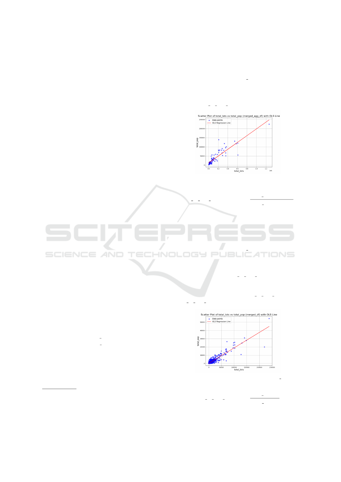
With the traditional integration methods, we ag-
gregate and integrate all selected datasets to the least
15
From dataset ”National Register of Condominiums”,
granularity level Geopoint-Date
16
From dataset ”Diplomas - Training in 2020”, granular-
ity level City-Year
common granularity level Department-Year. We can
get the scatter plot of sample data and the OLS line
(Figure 9) and the OLS regression result (Table 6).
Since the p-value of the total lots coefficient is less
than 0.01, the coefficient is not 0 in a 99% confidence
level. We confirm the relation between the two exist-
ing indicators. We can then construct a cross-theme
indicator pop to lots ratio
department
(Equation 7).
Figure 9: Plot and OLS Line with Traditional Integration.
pop to lots ratio
department
=
total pop
department
total lots
department
(7)
With our aggregation-union method, we first ag-
gregate and integrate the two datasets to their least
common granularity level City-Year. We can get the
scatter plot of sample data and the OLS line (Fig-
ure 10) and the OLS regression result (Table 7).
Since the p-value of the total lots coefficient is less
than 0.01, the coefficient is not 0 in a 99% confi-
dence level. We confirm the relation between the
two existing indicators. We can then construct a
cross-theme indicator pop to lots ratio
city
(Equation
8). Then, we aggregate the union to the granularity
level Department-Year in order to integrate it with the
third dataset. We aggregate pop to lots ratio
city
to
pop to lots ratio
department
(Equation 9).
Figure 10: Plot and OLS Line with Aggregation Union.
pop to lots ratio
city
=
total pop
city
total lots
city
(8)
Multi-Perspective Analyses of Spatio-Temporal Data About Well-Being
89

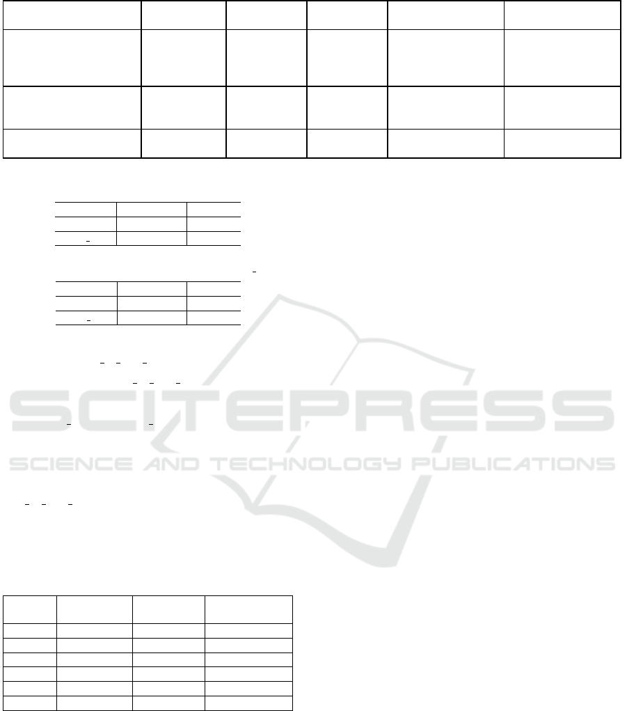
Table 5: Experimentation - Selected Datasets.
Source Theme
Spatial
granularity
Temporal
granularity
Spatial scope Temporal scope
National Register of
Condominiums
Domestic
environment
Geopoint Date
Department: ’11’,
’3’, ’32’, ...
startPoint =
’1900-01-01’,
endPoint =
’2024-06-30’
Diplomas - Training in
2020
Level of In-
dependence
City Year
Region:
’Grand-Est’,
’Occitanie’, ...
startPoint = ’2020’,
endPoint = ’2020’
Scholarship holders by
department
Level of In-
dependence
Department Year Country: ’France’
startPoint = ’2020’,
endPoint = ’2020’
Table 6: OLS regression result with Traditional Integration.
coefficient p-value
constant 1.191e+04 0.000
total lots 0.1869 0.000
Table 7: OLS regression result with Aggregation Union.
coefficient p-value
constant 96.3468 0.000
total lots 0.1875 0.000
pop to lots ratio
departement
= avg(pop to lots ratio
city
)
(9)
Although both methods show a strong relation be-
tween total lots and total pop, the OLS results are
different. We prefer the result with the aggregation-
union method because we have much more sample
data (plot) for the OLS.
Meanwhile, we can see a great difference between
pop to lots ratio
departement
constructed by the tradi-
tional method and by aggregation-union method (Ta-
ble 8). It shows how the integration granularity level
impacts the indicator construction.
Table 8: Result Comparison.
Region Department Traditional
Aggregation-
Union
1 971 0.756638 14.622511
2 972 0.655392 8.237147
3 973 1.815697 18.099793
4 974 0.916224 15.046275
11 75 0.177682 0.168966
... ... ... ...
Despite the relative simplicity of the traditional
method used to create the indicator, it is not highly
relevant. We calculated the ratio of the total popula-
tion to the total amount of dwellings in a department.
Since the population information in the raw data is
granular by City, we were assuming that the citizens
of different cities can move around the department at
will for housing. This is not realistic.
Our aggregation-union method, on the other hand,
considers the reality by assuming the citizens search
for housing in their own city. We first calculated
the ratio of the population to the total amount of
dwellings in each city, and then the average of this
ratio for each city in a department.
Compared to the traditional integration method
that agrees all datasets on a least common granular-
ity level at once, our integration model allows us to:
1. Have More and Finer Sample Data: When con-
firming the relation between two existing indica-
tors, the larger the sample data size, the more ac-
curate the correlation identification will be. We
can more convincingly confirm the statistical and
semantic correlation between two existing indica-
tors.
2. Constructing More Relevant Cross-Thematic
Indicators: When constructing new indicators,
the less aggregation processing an existing indi-
cator undergoes, the less its relevance will change.
Our method builds cross-theme indicators before
all data are aggregated to the same higher level of
precision, avoiding any change in the meaning of
existing indicators for cross-theme indicator con-
struction as much as possible.
6 CONCLUSIONS
In this paper, we introduced a conceptual model based
on a multi-perspective analysis framework of Well-
being with heterogeneous data sources. Recogniz-
ing the growing importance of Well-being as a mul-
tidimensional issue, we addressed the need for local
decision-makers to have access to a comprehensive
system that integrates various datasets from different
dimensions. We proposed an on-read data lake model
that stores diverse data without immediate processing.
The integration of data and the construction of indica-
tors start only when the requirement is present. This
approach minimizes the initial complexity of data in-
ENASE 2025 - 20th International Conference on Evaluation of Novel Approaches to Software Engineering
90

tegration, allowing for flexible and scalable analyses
based on user requirements.
Our modelling concept addresses two significant
challenges: the lack of multi-perspective analysis and
the complexity of handling heterogeneous datasets.
By proposing a novel data storage and integration ap-
proach, we create opportunities for more dynamic and
adaptable Well-being analysis. With the experimenta-
tion, we prove the feasibility of our concept and show
the superiority of our modelling approach.
The proposed model in the article lays the foun-
dation for future development. After proposing the
foundational model, the grounding and implementa-
tion of the model are subject to future work and fur-
ther exploration. To this end, our future work and de-
velopment directions are as follows:
• Realise the Construction of the Above Two
Zones: we will construct a data lake that meets
the requirements of the model concept proposed
in this paper. In the construction process, we
would like to integrate machine learning, deep
learning models, and other technologies to extract
the metadata for each zone quickly and accurately
and construct more practical cross-theme indica-
tors.
• Construct Analysis Model: We consider adopt-
ing the semantic trajectory model to construct an
analytical model that can describe and predict
the development trajectory of a certain territory.
Such a model would be able to describe the cur-
rent development in various aspects and reflect
the correlation between multiple themes. On the
other hand, it can predict future trends in well-
being based on historical data, enabling decision-
makers to take proactive measures.
• Develop Visualisation Tools: After building the
analysis model, we hope to develop an interac-
tive and user-friendly visualisation tool that al-
lows decision-makers to explore the data and anal-
ysis results more intuitively.
ACKNOWLEDGEMENTS
This article is particularly supported by Technop
ˆ
ole
DOMOLANDES.
REFERENCES
Ahmed Eldawy, Mostafa Elganainy, A. B. A. A. and Mok-
bel, M. (2017). Sphinx: Empowering impala for effi-
cient execution of sql queries on big spatial data. Ad-
vances in Spatial and Temporal Databases.
Ali Davoudian, L. C. and Liu, M. (2018). A survey on nosql
stores.
Anne De Biasi, Megan Wolfe, J. C. T. F. and Auerbach, J.
(2020). Creating an age-friendly public health system.
Innovation in Aging.
Arthur J. Reynolds, Judy A. Temple, S.-R. O. I. A. A. B. A.
B. W. (2011). School-based early childhood education
and age-28 well-being: Effects by timing, dosage, and
subgroups. Science.
Felix Gessert, Wolfram Wingerath, S. F. and Ritter, N.
(2017). Nosql database systems: A survey and de-
cision guidance. Comput Sci.
Khine, P. P. and Wang, Z. S. (2018). Data lake: A new
ideology in big data era. ITM Web of Conferences.
Le, Y. (2012). Challenges in data integration for spatiotem-
poral analysis. Journal of Map & Geography Librarie.
Luyi Bai, N. L. and Bai, H. (2021). An integration approach
of multi-source heterogeneous fuzzy spatiotemporal
data based on rdf. Journal of Intelligent & Fuzzy Sys-
tems.
Md Mahbub Alam, L. T. and Bifet, A. (2022). A survey on
spatio-temporal data analytics systems.
Nidzwetzki, J. K. and G
¨
uting, R. H. (2019). Demo paper:
Large scale spatial data processing with user defined
filters in bboxdb. 2019 IEEE International Conference
on Big Data (Big Data).
OECD (2011). How’s Life?: Measuring Well-Being.
OECD.
Patel, S. B. (2011). Analyzing urban layouts – can high
density be achieved with good living conditions? En-
vironment and Urbanization.
Ravat, F. and Zhao, Y. (2019). Data lakes: Trends and per-
spectives. pages 304–313.
Reardon, L. and Abdallah, S. (2013). Well-being and trans-
port: Taking stock and looking forward. Transport
Reviews.
Ryff, C. D. and Singer, B. H. (2008). Know thyself and
become what you are: A eudaimonic approach to psy-
chological well-being. Journal of Happiness Studies.
Wang, L. (2017). Heterogeneous data and big data analyt-
ics. Automatic Control and Information Sciences.
WHO (2023). National Programmes for Age-Friendly
Cities and Communities A Guide. WHO.
Xin Ding, Lu Chen, Y. G. C. S. J. and Bao, H. (2018).
Ultraman: A unified platform for big trajectory data
management and analytics. Proceedings of the VLDB
Endowment.
Zhang, Y. and Eldawy, A. (2020). Evaluating Computa-
tional Geometry Libraries for Big Spatial Data Ex-
ploration (GeoRich ’20). Association for Computing
Machinery.
Multi-Perspective Analyses of Spatio-Temporal Data About Well-Being
91