Predictive Regression Models of Machine Learning for Effort Estimation
in Software Teams: An Experimental Study
Wilamis K. N. Silva
1 a
, Bernan R. Nascimento
2 b
, P
´
ericles Miranda
3 c
and Emanuel P. Vicente
1 d
1
Cesar School Recife, Pernambuco, Brazil
2
Federal Institute of Piau
´
ı, Floriano, Brazil
3
Federal Rural University of Pernambuco, Recife, Brazil
Keywords:
Software Engineering, Software Team Effort Estimation, Evaluation Metrics, Machine Learning.
Abstract:
Estimating the effort required by software teams remains complex, with numerous techniques employed over
the years. This study presents a controlled experiment in which machine learning techniques were applied to
predict software team effort. Seven regression techniques were tested using eight PROMISE datasets, with
their performance evaluated across five metrics. The findings indicate that the XGBoost technique yielded
the best results. These results suggest that XGBoost is highly competitive compared to other established
techniques in the field. The paper proved to lay the foundation to guide future researchers in conducting
research in the field of software team effort estimation.
1 INTRODUCTION
Software effort estimation predicts the effort required
to complete a project successfully. The accuracy of
this estimation is directly proportional to the project’s
success (Goyal, 2022). Team effort estimation is criti-
cal during the project’s initial phase in software devel-
opment. Accurately identifying the amount of work
required leads to more realistic planning and directly
impacts resource allocation and the project’s timeline
(Jadhav et al., 2022). Team effort in software de-
velopment is an essential dimension that spans cru-
cial phases of planning and building software projects
(Sreekanth et al., 2023).
Team effort in software development is not merely
a quantitative matter but rather a qualitative inter-
action among the development team members, di-
rectly impacting the quality and efficiency of the soft-
ware development process (Jadhav et al., 2023). This
collaboration goes beyond the simple distribution of
tasks and involves aspects such as coordination, com-
munication, and knowledge sharing. With the in-
creasing robustness and scale of software projects,
the importance of an effective approach to manag-
a
https://orcid.org/0000-0002-8530-5916
b
https://orcid.org/0009-0001-0531-6042
c
https://orcid.org/0000-0002-5767-7544
d
https://orcid.org/0009-0008-9859-8819
ing team effort has grown, as it directly influences
project success (Sreekanth et al., 2023). Therefore,
accurately predicting this effort exerted by the devel-
opment team is essential for the early planning phases
of a software product.
According to the taxonomy proposed by (Boehm
et al., 2000), software estimation techniques can be
classified into the following categories: empirical
and composite, which encompass traditional tech-
niques based on data from previous projects; expert-
based, which focus on expert analysis and are often
used in conjunction with other techniques to correct
discrepancies; and machine learning-oriented. Ma-
chine learning-oriented techniques explore historical
domain data, using algorithms to formulate or infer
rules and/or models that predict future values. The
choice of using machine learning for software team
effort estimation is based on its adaptability, accuracy,
objectivity, and scalability, surpassing the limitations
of traditional methods and providing significant ben-
efits in time savings and delivery quality.
In this context, the following research question
emerged: How can the prediction of software team
effort estimation be improved through machine learn-
ing techniques? According to (Easterbrook et al.,
2008), the research question is classified as a com-
parative causal question. This inquiry aims to un-
derstand the causal relationship between variables by
comparing two or more groups or conditions. The
Silva, W. K. N., Nascimento, B. R., Miranda, P. and Vicente, E. P.
Predictive Regression Models of Machine Learning for Effort Estimation in Software Teams: An Experimental Study.
DOI: 10.5220/0013284800003929
Paper published under CC license (CC BY-NC-ND 4.0)
In Proceedings of the 27th International Conference on Enterprise Information Systems (ICEIS 2025) - Volume 2, pages 219-226
ISBN: 978-989-758-749-8; ISSN: 2184-4992
Proceedings Copyright © 2025 by SCITEPRESS – Science and Technology Publications, Lda.
219

philosophical paradigm that aligns with this study is
positivism. Positivism emphasizes the importance of
empirical observation, experimentation, and apply-
ing scientific methods for understanding and solving
problems (da Silva et al., 2010).
Although there are studies in the literature that
assess machine learning algorithms for software ef-
fort prediction, they frequently employ distinct exper-
imental methodologies, datasets, and evaluation met-
rics. This lack of standardization makes it challenging
to compare results across different research efforts.
To contribute in this direction, this article con-
ducted a controlled experimental study on the appli-
cation of machine learning techniques to predict the
effort estimation of software development teams us-
ing seven machine learning algorithms: J48 (Decision
Tree), KNN (K-Nearest Neighbors), SVM (Support
Vector Machine), ANN (Artificial Neural Network),
Bagging (Bootstrap Aggregating), Stacking (Stacked
Generalization), and XGBoost (Extreme Gradient
Boosting). To optimize the hyperparameters, the PSO
(Particle Swarm Optimization) technique was used.
The analyzed data comes from eight datasets from the
PROMISE repository, covering various specifications
and characteristics. The evaluation metrics used in-
clude MMR (Modified McCabe’s Complexity), MAE
(Mean Absolute Error), MdMRE (Magnitude Rela-
tive Error), and R2 score.
The article is organized as follows: Section 2 cov-
ers the related works. Section 3 discusses the method-
ology, and Section 4 provides the results and discus-
sions. Finally, section 5 presents the final considera-
tions.
2 RELATED WORK
The section presents some related work conducted by
professionals, academics, and researchers in the field
of software effort estimation and its impact on soft-
ware companies.
The work developed by (Tiwari and Sharma,
2022) applied machine learning techniques such as
SVM (linear, polynomial, RBF, sigmoid), Random
Forest, Stochastic Gradient Boosting, Decision Tree,
KNN (K-Nearest Neighbors), Logistic Regression,
Naive Bayes, and MLP to estimate effort in soft-
ware projects across various datasets, including IS-
BSG Release 12, Albrecht, China, COCOMO81, De-
sharnais, Finnish, Kemmerer, Kitchenham, Maxwell,
Miyazaki, NASA18, NASA93, and Telecom. The
study utilized evaluation metrics such as Pred (25),
Pred (50), MAE, MMRE, MMER, MdMRE, R-
Squared, MSE, and RMSE. Support Vector Regres-
sion (SVR) with an RBF kernel stood out, providing
the best results among the employed techniques. The
study did not utilize any hyperparameter optimization
techniques. Crucial factors, such as the scalability of
the algorithms, the high computational cost, and the
feasibility of implementation in development teams
with limited resources, were not thoroughly discussed
in the study.
Subsequently, the research developed by (Alham-
dany and Ibrahim, 2022) proposed the LASSO ma-
chine learning technique as a promising approach
for software development effort estimation, stand-
ing out from other algorithms in performance. Var-
ious techniques were utilized, such as Random For-
est (RF), Neural Networks (Neuralnet), Ridge Re-
gression (Ridge), Elastic Net (ElasticNet), Deep Neu-
ral Networks (Deepnet), Support Vector Machines
(SVM), Decision Trees (DT), and LASSO, on the
following datasets: China, Kemerer, Cocomo81,
Albrecht, Maxwell, Desharnais, and Kitchenham.
LASSO is notable for its ability to simplify models,
improve interpretability, address issues like overfit-
ting and multicollinearity, and perform automatic fea-
ture selection. redThe study offers a quantitative as-
sessment using metrics such as MAE, RMSE, and R-
squared, but could benefit from a deeper exploration
of the models’ interpretability in different project con-
texts.
The work by (Shukla and Kumar, 2023) investi-
gated different machine learning techniques and en-
semble models to predict Use Case Points (UCP),
aiming to improve software effort estimation. While
traditional methods like linear regression and deci-
sion trees have been widely used in previous stud-
ies, this work proposes the application of ensem-
bles, such as Boosting and Bagging, with different
base models, including SVR, MLP, and KNN. Among
the evaluated models, Boost-SVR demonstrated the
best performance, surpassing previous approaches in
metrics such as MAE, MSE, MBRE, and Pred(25),
demonstrating the effectiveness of ensemble tech-
niques in predicting UCP. The study utilized two pub-
lic datasets for estimating Use Case Points (UCP), re-
ferred to as DS1 and DS2, to conduct the experimen-
tal analysis. The study used Grid Search for hyper-
parameter optimization of the machine learning al-
gorithms. A drawback of Grid Search is that it can
be computationally costly and inefficient, especially
with large datasets or when there is a high number of
hyperparameters and possible combinations.
In (Saqlain et al., 2023), the authors utilized
five public datasets: ISBSG, NASA93, COCOMO81,
Maxwell, and Desharnais. The work included data
cleaning and selecting relevant features using Pear-
ICEIS 2025 - 27th International Conference on Enterprise Information Systems
220

son’s correlation coefficient. The applied machine
learning techniques included Linear Regression, Gra-
dient Boosting, Random Forest, and Decision Tree.
The best result was achieved using the R-squared (R²)
metric. The study did not consider the use of hy-
perparameter optimization techniques for the machine
learning algorithms.
Our article conducts an experimental analysis for
effort estimation in software development teams, us-
ing eight datasets from the PROMISE repository,
each with varied characteristics to ensure a robust
model evaluation. The algorithms applied include J48
(Decision Tree), KNN (K-Nearest Neighbors), SVM
(Support Vector Machine), ANN (Artificial Neural
Network), Bagging, Stacking, and XGBoost. Per-
formance evaluation was conducted through MMR
(Modified McCabe’s Complexity), MAE (Mean Ab-
solute Error), MdMRE (Median Relative Error), and
R² (Coefficient of Determination) metrics, allowing
for a detailed comparison of model accuracy and suit-
ability for the effort estimation problem. The arti-
cle stands out from previous work by incorporating
PSO (Particle Swarm Optimization) as a fine-tuning
method for hyperparameters in the machine learning
algorithms applied to effort estimation in software de-
velopment teams. The use of PSO is a significant ad-
vantage, as it offers an effective optimization strategy,
adaptively exploring the search space to find optimal
parameter combinations, which is not frequently ad-
dressed in the literature on software team effort esti-
mation.Table 1 presents the state-of-the-art compari-
son of related studies with our approach.
3 EXPERIMENTAL
METHODOLOGY
This section details the proposed experimental
methodology for conducting the experiments. The
methodology was structured to ensure the validity and
reproducibility of the results and to enable an in-depth
analysis of machine learning techniques. The study
methodology consists of three main stages. First, the
dataset undergoes a cross-validation step, which di-
vides it into training and test subsets, allowing for a
robust assessment of the model’s performance and re-
ducing overfitting issues. Next, in the second stage,
the regression model is trained using the training data.
During this process, a specific optimization, called
PSO (Particle Swarm Optimization), is used to adjust
the model’s hyperparameters and improve its perfor-
mance. Finally, in the third stage, the trained model
is evaluated using specific metrics to verify its accu-
racy and effectiveness, which enables a quantitative
analysis of the model’s performance on the test data.
This methodological flow allows for rigorous opti-
mization and evaluation, promoting a systematic and
well-founded analysis of the results, as illustrated in
Figure 1.
3.1 Datasets
The study utilized different datasets from the
PROMISE (Predictive Models in Software Engineer-
ing) repository across various application domains.
The characteristics and specifications of the datasets
used during the experiments are described below. Ta-
ble 2 presents some features of the datasets, such as
the number of examples, numerical attributes, and the
output unit.
Choosing datasets from the PROMISE repository
ensured a comprehensive and robust analysis of ma-
chine learning techniques in software development ef-
fort estimation. It is important to note that the datasets
underwent no normalization process.
Data preprocessing involved applying Outlier
Correction (Capping) and Outlier Removal using the
Interquartile Range (IQR) method to the datasets used
in the experiments. Capping was employed to limit
the impact of outliers while retaining them in the
dataset, whereas IQR aimed to exclude unwanted ob-
servations.
3.2 Evaluation Metrics
There are various metrics in the literature for evalu-
ating the techniques’ performance on software team
effort estimation; however, in this study, we used the
following metrics: MMR (Modified McCabe’s Com-
plexity) (Fenton and Bieman, 2014), MAE (Mean
Absolute Error) (Hammad and Alqaddoumi, 2018),
MdMRE (Magnitude Realative Error) (Corr
ˆ
ea et al.,
2020), and R
2
score (Saqlain et al., 2023). These met-
rics were chosen to provide a comprehensive eval-
uation of model performance in team effort estima-
tion for software projects. MMR (Modified McCabe’s
Complexity) was used to assess system complexity,
as it provides insights into maintainability and failure
risk, which is particularly relevant in projects where
complexity may impact the effort required for mainte-
nance and development. MAE (Mean Absolute Error)
evaluates the model’s average accuracy by calculating
the mean of absolute errors without amplifying large
errors; this makes it an interpretable and relevant met-
ric for effort estimation, as it reflects the average error
directly. MdMRE (Magnitude Relative Error) mea-
sures relative error and is widely used in the software
effort estimation literature. This metric allows for
Predictive Regression Models of Machine Learning for Effort Estimation in Software Teams: An Experimental Study
221

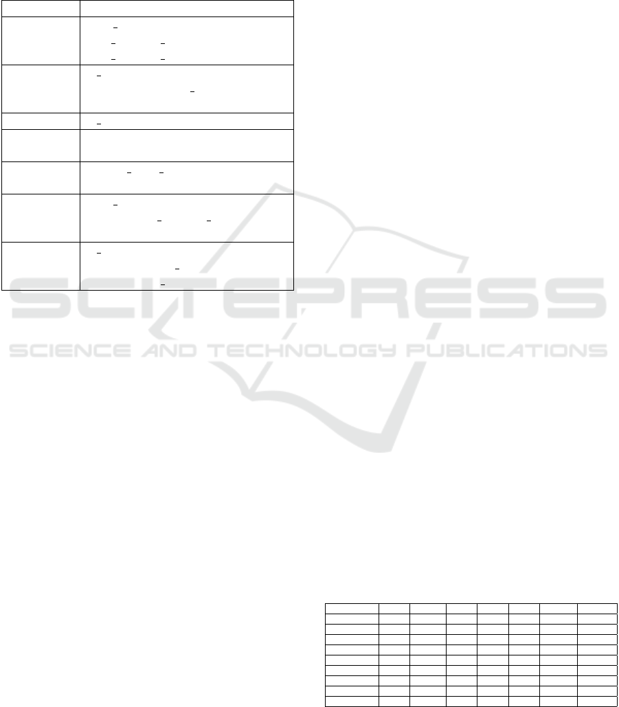
Table 1: State-of-the-Art Comparison of Related Studies.
Ref Datasets Models Metrics Hyperparameter Op-
timization
(Tiwari and Sharma, 2022) Albrecht, China,
COCOMO81,
Desharnais,
Finnish, Kem-
merer, Kitchen-
ham, Maxwell,
Miyazaki,
NASA18,
NASA93 Tele-
com
Support Vector Machines
with linear, polynomial,
RBF, and sigmoid ker-
nels, Random Forest,
Stochastic Gradient
Boosting, Decision Tree,
K-Nearest Neighbors,
Logistic Regression,
Naive Bayes, Multi-Layer
Perceptron
Pred (25), Pred (50),
MAE, MMRE, MMER,
MdMRE,R-Squared,
MSE, RMSE
None
(Alhamdany and Ibrahim, 2022) China, Kemerer,
Cocomo81, Al-
brecht, Maxwell,
Desharnais,
Kitchenham
Random Forest, SVM
(Support Vector Machines
), Decision Tree, Neural
Networks, Ridge Regres-
sion, LASSO Regression,
ElasticNet Deepnet
MAE, RMSE, R-
Squared
None
(Shukla and Kumar, 2023) Usp, Usp05-tx,
NASA, CO-
COMO81, SDR,
China, and De-
sharnais
Weka tool for estimation MAE, Pred, Correla-
tion Coefficient, RRSE,
MMRE, RAE
Grid Search
(Saqlain et al., 2023) ISBSG,
NASA93, CO-
COMO81,
Maxwell, De-
sharnais
Linear Regression, Gra-
dient Boosting, Random
Forest, Decision Tree
R², RMSE None
Proposed Method Albrecht, China,
COCOMO81,
Desharnais,
Finnish, Kitchen-
ham, Kemerer,
Maxwell
J48 (Decision Tree), KNN
(K-Nearest Neighbors),
SVM (Support Vector
Machine), ANN (Arti-
ficial Neural Network),
Bagging (Bootstrap
Aggregating), Stacking
(Stacked Generalization),
XGBoost (Extreme Gra-
dient Boosting)
MMRE, MAE,
MDMRE, R
2
PSO (Particle Swarm
Optimization)
Figure 1: Methodological process of the study.
method comparisons and assesses the model’s con-
sistency across different estimation scenarios. R² (co-
efficient of determination) indicates the proportion of
variance explained by the model, offering insight into
how much of the data variability is captured, which
is essential to evaluate the model’s overall suitability,
especially in datasets with high variability. Each met-
ric was therefore chosen to cover different evaluation
aspects, from accuracy to the impact of deviations and
system complexity. Each metric’s mathematical for-
mulation and description are presented in formulas 1,
2, 3, and 4.
A) MMR (Modified McCabe’s Complexity). Based
on the idea of summing the McCabe complexity of
ICEIS 2025 - 27th International Conference on Enterprise Information Systems
222

Table 2: Description of Databases.
Dataset Nº of Examples Nº of Numeric Attributes Output Unit
Albrecht 12 24 Person-Months
China 19 499 Person-Hours
COCOMO81 17 63 Person-Months
Desharnais 12 81 Person-Months
Finnish 9 38 Person-Months
Kitchenham 10 145 Person-Hours
Kemerer 8 15 Person-Months
Maxwell 27 62 Person-Hours
each method, which is the count of the number of in-
dependent paths through a method in a program. A
lower result in the MMR metric is generally consid-
ered better. The MMR is calculated as follows:
MMR =
n
∑
i=1
(CC
i
+ 1) (1)
where:
• CC
i
is the McCabe complexity of the method i,
• n is the total number of methods in the software,
• A lower result in the MMR metric is generally
considered better.
B) MAE (Mean Absolute Error). It sums the mean of
all absolute errors. The smaller the presented value,
the better the metric. The MAE is calculated as fol-
lows:
MAE =
1
n
n
∑
i=1
|y
i
− ˆy
i
| (2)
where:
• n is the total number of observations,
• y
i
are the actual values,
• ˆy
i
are the predicted values,
• The smaller the presented value, the better the
metric.
C) MdMRE (Magnitude Relative Error). According
to (Corr
ˆ
ea et al., 2020), the metric Median Magnitude
of Relative Error (MdMRE) represents the median of
the Magnitude of Relative Error (MRE). MdMRE is
an error metric that provides an overview of model
accuracy by assessing the magnitude of discrepancies
between predictions and actual values. Overestimated
values less influence this metric, as it considers the
median of the dataset, with lower values indicating
better results. Equation 3 presents the mathematical
formulation of the MdMRE metric.
MdMRE =
1
n
n
∑
i=1




y
i
− ˆy
i
y
i




× 100 (3)
where:
• n is the total number of observations,
• y
i
are the real values,
• ˆy
i
are the predicted values.
D) R
2
score. The metric provides an indication of the
proportion of variance in the dependent variable that
is predictable from the independent variables. The
closer the value of the R
2
score is to 1, the better the
model fits the data.
• 0 indicates that the model cannot explain the vari-
ability of the data,
• 1 indicates that the model perfectly explains the
variability of the data.
The R
2
is calculated as follows:
R
2
= 1 −
SS
res
SS
tot
(4)
where:
• SS
res
is the sum of the squares of the residuals (the
differences between the observed values and the
predicted values),
• SS
tot
is the total sum of squares (the differences
between the observed values and the mean of the
observed values).
3.3 Configuration of the Experiments
For each dataset presented in Table 2, the follow-
ing machine learning regression techniques were ap-
plied: J48 (Decision Tree), KNN (K-Nearest Neigh-
bors), SVM (Support Vector Machine), ANN (Arti-
ficial Neural Network), Bagging (Bootstrap Aggre-
gating), Stacking (Stacked Generalization), and XG-
Boost (Extreme Gradient Boosting). The selection
of machine learning techniques was based on various
factors. Firstly, these techniques are widely recog-
nized and accepted in the scientific community, with
a vast amount of research and validation across differ-
ent domains, demonstrating their good performance
in regression tasks. Each technique offers its advan-
tages, contributing to a more comprehensive analy-
sis and enhancing the reliability and accuracy of pre-
dictions. By employing various methods, the study
benefits from diverse analytical perspectives and pre-
dictive capabilities, which can result in a robust fi-
nal model. Finally, previous experiences and studies
indicating the success of these approaches in similar
problems also motivated their inclusion.
All algorithms had their hyperparameters (see Ta-
ble 3) optimized by the PSO (Particle Swarm Opti-
mization), chosen for its effectiveness in finding hy-
perparameter combinations that maximize the perfor-
mance of machine learning models. For each algo-
rithm, the PSO configurations included a fixed num-
ber of particles set at 30 and a maximum number of
Predictive Regression Models of Machine Learning for Effort Estimation in Software Teams: An Experimental Study
223

iterations limited to 100. The adopted fitness function
is the Mean Absolute Error (MAE), and the learning
parameters were defined according to standard set-
tings. Table 3 presents the hyperparameters of each
algorithm considered for optimization and details the
parameters interval of each.
Table 3: Description of Algorithm Hyperparameters.
Algorithm Hyperparameter Description
J48 max depth ranges from 1 to 20,
min samples split from 2 to 50, and
min samples leaf from 1 to 10
Bagging n estimators varies between 1 and
100, while max samples ranges
from 0.1 to 1
KNN n neighbors is set from 1 to 50
SVM C is tuned between 0.1 and 100, and
epsilon between 0.001 and 1
ANN hidden layer size ranges from 10 to
100 and alpha from 0.0001 to 1
Stacking max depth is tuned between 1 and
20, and min samples split between
2 and 50
Xgboost n estimators ranges from 10 to
1000, learning rate from 0.01 to
0.3, and max depth from 1 to 10
All experiments were conducted using the cross-
validation methodology with 10 folds. According
to the literature, using cross-validation with different
numbers of folds is a common practice in machine
learning experiments to explore how model perfor-
mance varies with different data split configurations.
For model creation, we used the open-source web-
based application Jupyter Notebook, along with the
scikit-learn library, version 1.5.2. Jupyter Notebook
is a Python-based development environment that al-
lows readers and researchers to create and assess the
validity of results under different data and model as-
sumptions (Kluyver et al., 2016).
3.4 Statistical Analysis
For the statistical analysis of the results obtained by
different machine learning techniques, the Friedman
test (α = 0.05) was applied for global comparisons
of the algorithms, followed by the Durbin-Conover
post-hoc test for pairwise comparisons. This test was
chosen for its robustness in situations where data do
not follow a normal distribution, making it particu-
larly useful in comparing the performance of machine
learning techniques applied to the same dataset.
In the study, the null hypothesis (H
0
) assumed
no significant difference between the models’ average
rankings, meaning that all methods exhibit equivalent
performance. The alternative hypothesis (H
1
), on the
other hand, suggests that at least one of the methods
significantly differs from the others in terms of per-
formance.
4 RESULTS AND DISCUSSIONS
Table 4 compares the MMR metric across algorithms
applied to different datasets, highlighting XGBoost as
the best overall choice due to its lowest average MMR
(0.3849) and consistent performance. J48 (average
MMR = 0.4395) and KNN (average MMR = 0.4254)
demonstrated similar performance, being suitable for
smaller and more structured datasets, while SVM (av-
erage MMR = 0.4309) showed stability, particularly
in scenarios requiring consistent results. In contrast,
Bagging (average MMR = 0.6698) and Stacking (av-
erage MMR = 0.6244) exhibited higher variability.
ANN showed the highest average MMR (8.5413),
heavily impacted by outliers, indicating lower suit-
ability. Therefore, XGBoost is recommended for
greater reliability, with J48, KNN, and SVM as viable
alternatives in specific contexts. The selection of the
algorithm should consider the dataset characteristics
to achieve optimal performance.
The Friedman test was applied, yielding p −
value = 0.064, indicating insufficient evidence to
claim that one algorithm performs consistently bet-
ter than the others. The results of the Durbin-
Conover test indicate that the Stacking algorithm
exhibited significant differences compared to J48,
KNN, SVM, and XGBoost, particularly in compar-
ison with XGBoost (p − value = 0.003), suggesting
a distinct performance behavior. XGBoost also ex-
hibited significant differences compared to Bagging
(p − value = 0.040), indicating a differentiated er-
ror structure. In contrast, most algorithms, such as
J48, KNN, SVM, and ANN, did not show significant
differences among themselves, suggesting that they
could be interchangeable without substantial perfor-
mance impact.
Table 4: Performance of Algorithms on Different Datasets
for the MMR Metric.
Dataset J48 Bagging KNN SVM ANN Stacking XGBoost
albretch 0.301 0.333 0.425 0.294 0.864 0.358 0.304
china 0.121 0.102 0.129 0.208 0.106 0.156 0.101
cocomo81 1.274 1.373 1.167 0.693 0.744 2.132 1.057
desharnais 0.225 0.298 0.263 0.270 57.003 0.282 0.245
finnish 0.021 0.016 0.011 0.012 8.395 0.034 0.014
kemerer 0.583 0.800 0.656 0.428 0.548 0.677 0.515
kitchenham 0.273 0.277 0.263 0.362 0.304 0.373 0.315
maxwell 0.718 2.159 0.489 1.180 0.362 0.983 0.528
average MMR 0.4395 0.6698 0.6698 0.4309 8.5413 0.6244 0.3849
ICEIS 2025 - 27th International Conference on Enterprise Information Systems
224

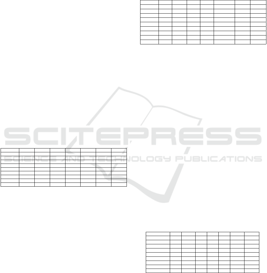
Table 5 presents the performance of algorithms
using the MAE metric. Stacking emerged as the
best overall choice with the lowest average MAE
(183.702,18), demonstrating consistent performance
across various datasets, such as finnish (0.376) and
desharnais (0.485). The XGBoost (average MAE=
228.363,39) and KNN (average MAE= 227.449,12)
showed similar performance, serving as viable alter-
natives when Stacking is not applicable. J48 (aver-
age MAE= 257. 148,88) performed well on smaller
datasets, such as finnish (0.141), but was less effi-
cient on larger datasets. The ANN (average MAE=
295.703,95) had its average inflated by extreme val-
ues in datasets like maxwell (2.364,448), compromis-
ing its overall efficiency. Meanwhile, Bagging (av-
erage MAE= 330.344,55) and SVM (average MAE=
360.511,45) showed the highest average MAE values,
indicating lower suitability for the evaluated datasets.
The Friedman test was applied, resulting in a
p − value = 0.329, showing insufficient evidence to
reject the null hypothesis that all algorithms have
similar performance. Applying the Durbin-Conover
method, only the comparison between Stacking and
XGBoost produced a p − value = 0.018, indicating a
statistically significant difference between these mod-
els.
Table 5: Performance of Algorithms on Different Datasets
for the MAE Metric.
Dataset J48 Bagging KNN SVM ANN Stacking XGBoost
albretch 117.000 129.884 143.350 122.379 397.767 129.450 117.768
china 138.490 125.492 128.708 243.858 123.736 180.554 103.491
cocomo81 56.267 59.271 61.789 50.421 50.556 71.563 48.282
desharnais 0.271 0.381 0.369 0.393 89.665 0.485 0.348
finnish.csv 0.141 0.136 0.082 0.087 97.296 0.376 0.112
kemerer 97.055 71.990 106.605 63.209 64.827 97.625 78.761
kitchenham 363.825 369.265 352.080 488.233 359.781 470.410 392.378
maxwell 2.056,418 2.642,000 1.818,800 2.883,123 2.364,448 1.468,667 1.826,166
average MAE 257.148,88 330.344,55 227.449,12 360.511,45 295.703,95 183.702,18 228.363,39
Table 6 presents the performance of the algorithms
using the R² metric. XGBoost stood out with the high-
est average R² (1.0597), proving to be the most effec-
tive and consistent algorithm among those evaluated.
Its superiority is evident in datasets such as china
(0.986) and finnish (0.801), where it achieved high
values close to the ideal. Stacking also performed
well, with an average R² of 0.7882, achieving positive
results in china (0.950) and finnish (0.646), indicating
that it is a viable alternative in many scenarios. ANN
presented the worst average R² (-9.169,704), heav-
ily influenced by extreme outliers in the desharnais (-
7.006,388) and finnish (-48.011,819) datasets. Based
on these results, XGBoost is recommended as the best
overall choice due to its consistent and high perfor-
mance. Stacking is a promising alternative, while
algorithms such as SVM, J48, Bagging, and KNN
should only be considered in specific scenarios.
The Friedman test yielded a p − value = 0.786,
providing insufficient evidence to reject the null hy-
pothesis. This result indicates that there is no statisti-
cally significant difference in performance among the
algorithms analyzed, according to this test.
Table 6: Performance of Algorithms on Different Datasets
for the R² Metric.
Dataset J48 Bagging KNN SVM ANN Stacking XGBoost
albretch -1.009 -1.392 -2.538 -1.097 -15.672 -1.536 -1.207
china 0.968 0.980 0.980 0.820 0.980 0.950 0.986
cocomo81 -5.144 -7.682 -12.473 -1.470 -0.286 -4.253 -4.898
desharnais -0.098 -1.154 -0.322 -0.267 -70063388 -0.290 0.131
finnish 0.791 0.922 0.914 0.925 -48011819 0.646 0.801
kemerer nan nan nan nan nan nan nan
kitchenham 0.755 0.772 0.792 0.658 0.812 0.706 0.749
maxwell nan nan nan nan nan nan nan
average R² -0.6228 -1.2590 -2.1078 -0.0718 -9.169.704,00 0.7882 1.0597
Table 7 presents the performance of the algo-
rithms using the MDMRE metric. The analysis of
the average results reveals that SVM achieved the
best overall performance, with the lowest average
MDMRE (0.2584), standing out as the most efficient
choice for the evaluated datasets. XGBoost demon-
strated the second-best performance, with an average
of 0.2696, proving to be a viable alternative to SVM.
This algorithm achieved particularly competitive re-
sults in datasets such as china (0.072) and finnish
(0.014), confirming its effectiveness. Stacking (aver-
age MDMRE = 0.2954) and KNN (average MDMRE
= 0.3058) also showed reasonable performance, with
low and consistent values across various datasets.
Bagging (average MDMRE = 0.3168) and J48 (av-
erage MDMRE = 0.3231) exhibited intermediate per-
formance, with higher values in some datasets, such
as cocomo8 and maxwell, indicating greater variabil-
ity in results and lower precision in certain scenarios.
On the other hand, ANN showed the worst overall
performance, with an average MDMRE of 0.6548.
The Friedman test yielded a p − value = 0.282,
indicating that there is no statistically significant dif-
ference among the algorithms.
Table 7: Performance of Algorithms on Different Datasets
for the MDMRE Metric.
Dataset J48 Bagging KNN SVM ANN Stacking XGBoost
albretch 0.283 0.292 0.354 0.275 0.711 0.294 0.276
china 0.106 0.090 0.111 0.156 0.093 0.137 0.092
cocomo81 0.616 0.570 0.593 0.503 0.549 0.718 0.483
desharnais 0.194 0.256 0.221 0.239 1.377 0.259 0.220
finnish 0.024 0.015 0.011 0.012 1.319 0.034 0.014
kemerer 0.549 0.445 0.505 0.358 0.291 0.528 0.435
kitchenham 0.238 0.233 0.228 0.295 0.251 0.312 0.256
maxwell 0.555 0.643 0.416 0.693 0.349 0.624 0.401
average MDMRE 0.3231 0.3168 0.3058 0.2584 0.6548 0.2954 0.2696
5 CONCLUSIONS
This study addressed the research question: ”How
can software team effort estimation prediction be im-
proved through machine learning techniques?” The
Predictive Regression Models of Machine Learning for Effort Estimation in Software Teams: An Experimental Study
225

study conducted a controlled experimental analysis
utilizing eight machine learning techniques to predict
software team effort, evaluated based on comprehen-
sive metrics such as MMR, MAE, MdMRE, and R².
While statistical results indicate that multiple algo-
rithms may be applicable in different scenarios with-
out significant losses in accuracy, the research identi-
fied XGBoost as the best overall performer. It demon-
strated superior performance across several metrics
due to its high computational efficiency, leveraging
optimization techniques such as parallel processing
and caching to accelerate training. Furthermore, XG-
Boost is less sensitive to outliers owing to its use of
a regularized cost function that balances data fitting
and model simplicity. The use of hyperparameter op-
timization techniques, such as Particle Swarm Opti-
mization (PSO), significantly contributed to improv-
ing the obtained results.
Additionally, the study identified that algorithms
such as Stacking and KNN are also promising in spe-
cific scenarios, while others, such as Artificial Neural
Networks (ANN), face limitations due to their sensi-
tivity to outliers. This underscores the importance of
careful algorithm selection, considering the character-
istics and complexity of the data used.
For future research, we recommend exploring ad-
vanced preprocessing strategies and creating larger
and more diverse datasets capable of reflecting the
variability and complexity of real-world data. Fur-
thermore, evaluating the application of hybrid tech-
niques that combine the strengths of different algo-
rithms could further enhance the robustness and ac-
curacy of effort estimations. It is anticipated that the
findings of this study will contribute to advancing the
field.
REFERENCES
Alhamdany, F. B. and Ibrahim, L. M. (2022). Software
development effort estimation techniques: A survey.
Journal of Education and Science, 31(1):80–92.
Boehm, B., Abts, C., and Chulani, S. (2000). Software de-
velopment cost estimation approaches—a survey. An-
nals of software engineering, 10(1):177–205.
Corr
ˆ
ea, W. A. et al. (2020). Applying machine learning for
effort estimation in software development. Master’s
Thesis, S
˜
ao Lu
´
ıs - MA, Brazil.
da Silva, F., Santos, A., Soares, S., Franc¸a, A., and Mon-
teiro, C. (2010). Six years of systematic literature re-
views in software engineering: an extended tertiary
study. In 32th international conference on software,
ICSE, volume 10, pages 1–10.
Easterbrook, S., Singer, J., Storey, M.-A., and Damian, D.
(2008). Selecting empirical methods for software en-
gineering research. Guide to advanced empirical soft-
ware engineering, pages 285–311.
Fenton, N. and Bieman, J. (2014). Software metrics: a rig-
orous and practical approach. CRC press.
Goyal, S. (2022). Effective software effort estimation using
heterogenous stacked ensemble. In 2022 IEEE Inter-
national Conference on Signal Processing, Informat-
ics, Communication and Energy Systems (SPICES),
volume 1, pages 584–588. IEEE.
Hammad, M. and Alqaddoumi, A. (2018). Features-level
software effort estimation using machine learning al-
gorithms. In 2018 international conference on innova-
tion and intelligence for informatics, computing, and
technologies (3ict), pages 1–3. IEEE.
Jadhav, A., Kaur, M., and Akter, F. (2022). Evolution of
software development effort and cost estimation tech-
niques: five decades study using automated text min-
ing approach. Mathematical Problems in Engineer-
ing, 2022:1–17.
Jadhav, A., Shandilya, S. K., Izonin, I., and Gregus, M.
(2023). Effective software effort estimation enabling
digital transformation. IEEE Access.
Kluyver, T., Ragan-Kelley, B., P
´
erez, F., Granger, B. E.,
Bussonnier, M., Frederic, J., Kelley, K., Hamrick,
J. B., Grout, J., Corlay, S., et al. (2016). Jupyter
notebooks-a publishing format for reproducible com-
putational workflows. Elpub, 2016:87–90.
Saqlain, M., Abid, M., Awais, M., Stevi
´
c,
ˇ
Z., et al.
(2023). Analysis of software effort estimation by ma-
chine learning techniques. Ing
´
enierie des Syst
`
emes
d’Information, 28(6).
Shukla, S. and Kumar, S. (2023). Towards ensemble-based
use case point prediction. Software Quality Journal,
31(3):843–864.
Sreekanth, N., Rama Devi, J., Shukla, K. A., Mohanty, D.,
Srinivas, A., Rao, G. N., Alam, A., and Gupta, A.
(2023). Evaluation of estimation in software devel-
opment using deep learning-modified neural network.
Applied Nanoscience, 13(3):2405–2417.
Tiwari, M. and Sharma, K. (2022). Comparative analysis of
estimation of effort in machine-learning techniques.
International Journal of Advanced Research in Sci-
ence, Communication and Technology, 3(2):17–23.
ICEIS 2025 - 27th International Conference on Enterprise Information Systems
226