Dynamic Charging on the Go: Optimizing Mobile Charging Stations for

Electric Vehicle Infrastructure

Suhas Jain and Arobinda Gupta

Dept. of Computer Science & Engineering, Indian Institute of Technology Kharagpur, WB-721302, India

Keywords:

Electric Vehicle, Mobile Charging Station, Charging Request, Scheduling.

Abstract:

With the growing adoption of electric vehicles (EVs) as an eco-friendly and sustainable means of transporta-

tion, availability of adequate EV charging infrastructure has become very important. While ﬁxed charging

stations are the primary means for public charging, they can be effectively augmented by mobile charging

stations. In this paper, we address the problem of planning and operating a mobile charging station ﬂeet by an

operator. We propose an algorithm for the operator to use for route planning of the MCSs and for scheduling

charging requests of EVs to them to try to maximize the number of charging requests served. Detailed simu-

lation results are presented in different realistic scenarios to show that the proposed algorithm works well.

1 INTRODUCTION

Electric vehicles (EVs) are being increasingly seen as

the future of transportation towards a more sustain-

able future, with the global EV market growing at

a fast rate. EVs are primarily charged at home us-

ing slow charging options, or at ﬁxed charging sta-

tions (FCSs) installed at designated locations offering

fast charging options. As the adoption of EVs grows,

the availability and accessibility of adequate charging

points will become pivotal factors in the widespread

acceptance of EVs. However, ﬁxed charging stations

are anchored to speciﬁc locations, which presents a

number of challenges, such as lack of universal ac-

cessibility, space availability, high setup cost etc.

Mobile charging stations (MCSs) have been pro-

posed as a versatile and innovative solution to these

challenges. MCSs can be built using conventional

vehicles carrying batteries for charging, with plug-

in charging capabilities for EVs to charge. They can

park anywhere with enough space to charge EVs, and

can bring charging facilities directly to the EV user,

regardless of their locations, thereby providing easy

access to EV charging. MCSs can be swiftly de-

ployed to areas experiencing high demand or in ar-

eas where the charging infrastructure is inadequate or

overloaded. They can also be used to provide emer-

gency charging services to stalled vehicles with little

or no charge left.

In this paper, we consider an MCS operator with

a ﬂeet of MCSs, and address the problem of dispatch-

ing the MCSs to different locations in a city to serve

EV charging requests. Speciﬁcally, we ﬁrst formu-

late the problem of planning the placement of MCSs

at different locations in a city and scheduling EVs to

a suitable MCS for charging. We then propose an al-

gorithm called GoMCS for the problem that attempts

to maximize the number of requests served while try-

ing to optimize average distance travelled by MCSs

and average waiting times of EVs. Detailed simula-

tion results are presented to show that the proposed

algorithm performs well compared to an existing al-

gorithm.

2 RELATED WORK

The existing literature in the area of mobile EV charg-

ing can be broadly classiﬁed into two parts, design

of MCS infrastructure, and dispatch and operation

of MCSs (the focus of this work). Several existing

works have looked at different aspects of MCS dis-

patch and operation such as path planning, deciding

priority of EVs to be charged, deciding charging lo-

cations and times etc., to optimize various objectives

such as serving the most number of customers, mini-

mizing wait time for customers, maximizing proﬁt for

MCS operators etc. (Atmaja and Mirdanies, 2015;

Cui et al., 2018; Tang et al., 2020; Raboaca et al.,

2020; Moghaddam et al., 2021; Jeon and Choi, 2021;

Kong, 2019; El-Fedany et al., 2021; Zhang et al.,

466

Jain, S. and Gupta, A.

Dynamic Charging on the Go: Optimizing Mobile Charging Stations for Electric Vehicle Infrastructure.

DOI: 10.5220/0013286400003941

Paper published under CC license (CC BY-NC-ND 4.0)

In Proceedings of the 11th International Conference on Vehicle Technology and Intelligent Transport Systems (VEHITS 2025), pages 466-473

ISBN: 978-989-758-745-0; ISSN: 2184-495X

2020; Liu et al., 2022; Wang et al., 2019; Liu et al.,

2018). The algorithms differ in assumptions made

and target parameters chosen.

Among the works mentioned above, only (Liu

et al., 2018) and (Tang et al., 2020) address online

route planning and operation of MCSs. The work

in (Liu et al., 2018) focus on using demand and dis-

tance based routing algorithms for MCSs, but does

not propose any mechanism for ﬁnding the optimal

MCS for a particular request. The work in (Tang

et al., 2020) formulates the problem as a mixed in-

teger linear programming problem which is not scal-

able to a large number of requests and MCSs. We

aim to build efﬁcient heuristic algorithms which per-

form both route planning of MCSs and scheduling of

charging requests in an online manner at scale.

3 PROBLEM SPECIFICATION

We consider EVs moving in a city, with an MCS op-

erator providing mobile charging service to the EVs.

MCSs are charging stations with limited charge ca-

pacity (from batteries carried on vehicles) that move

within the city. Their states are always known to the

MCS operator, including remaining charge, location,

and availability. While the capacity of an MCS to

charge EVs depends on the capacity of batteries it car-

ries, the MCS itself is assumed to be gas-powered;

hence, it is assumed to have no range limitation for

its own movement. An MCS can only charge EVs at

one or more of a set of predeﬁned ﬁxed charging loca-

tions. We assume that at a time, only one MCS can be

parked at one of these locations. The charging service

is provided for a ﬁxed duration in a day, broken up

into T time instants. At the start of a day, all MCSs

are fully charged and stationed at their home depot.

MCSs travel to different locations to charge EVs as

directed by the MCS operator. If an MCS runs out of

charge, it goes to its closest depot to get charged, and

then services requests again.

Each EV move from a source to a destination lo-

cation. If the remaining charge is deemed to be insuf-

ﬁcient, EVs make charging requests with details of

their requirements to the MCS operator’s central con-

trol system. The central system sends a response to

the request immediately accepting or rejecting it. If

the system accepts a request, it is always served.

The road network in the city is modeled as a di-

rected graph G = (N , E), where N denotes the set

of nodes, and E denotes the set of roads. The nodes

can be vehicle locations, charging stations, depot lo-

cations, charging locations, or source/destination lo-

cations.

The set of electric vehicles is denoted as V .

A vehicle v ∈ V is represented by the tuple

⟨cap

, soc

, loc

, s

, d

, c

⟩, where cap

is the bat-

tery capacity (kWh) of v, soc

is the state of charge

(SoC) of v at time t (charge remaining as a percentage

of total charge), loc

is the location of v at time t, s

the average speed of the vehicle, d

is the discharging

rate (battery discharged per unit distance), and c

the charging rate (battery charged per unit time).

Let M be the set of all MCSs. An MCS m ∈ M

at a particular time t, is represented by the tuple

⟨ dep

, cap

, soc

, loc

, s

, out

, c

, cout

req list

, path

⟩, where dep

is the home depot of

m, cap

is the effective battery capacity (kWh) of m

(to charge EVs), soc

is the state of charge (SoC) of

m, loc

is the location of m at time t, s

is the av-

erage speed of m, out

is the number of outlets/ports

in m which can be used for charging, c

is the rate at

which m can get charged, cout

is the rate at which m

can charge a vehicle (in kWh per unit time), path

the future path planned for m at time t (a sequence of

tuples, each with a location, starting time and ending

time denoting the duration the MCS will stay in that

location), and req

list

is the requests scheduled at

the MCS at time t. The requests are stored as an array

of 2-tuples, containing the starting time at which the

vehicle is scheduled to start, and the time at which the

charging will end.

Let R be the set of all charging requests.

A request r ∈ R is represented by the tuple

⟨ time

, v

, curr soc

, des soc

, req loc

des loc

, dev

, wait

⟩, where time

is the time at

which the request is made, v

is the EV which has

made the request, curr soc

is the current SoC of the

EV requesting charge, des soc

is the desired SoC of

the EV requesting charge, req loc

is the current lo-

cation of the EV when the request is made, des loc

is the destination location of the EV, dev

is the max-

imum extra distance the EV is willing to travel for

charging, and wait

is the maximum time the vehicle

can wait at the charging location. Let L (L ⊂ N ) be

the set of all charging locations. MCSs can charge

EVs only at one of these locations.

The output of any algorithm for the MCS alloca-

tion problem is a |M |×|V |×|L|×T matrix S , where

S[m, v, l, t] = 1 if and only if MCS m is charging the

EV v placed at charging location l at time t, 0 other-

wise. The problem is to compute a schedule for plac-

ing the set of MCSs at the set of locations for charging

the vehicles in the set V such that the number of ve-

hicles charged is maximized. Formally, the goal is to

maximize

∑

m∈M

∑

v∈V

∑

l∈L

∑

t∈T

Dynamic Charging on the Go: Optimizing Mobile Charging Stations for Electric Vehicle Infrastructure

467

(S[m, v, l, t] = 0 ∩ S[m, v, l, t + 1] = 1)

subject to the following constraints:

1. An EV can be in at most one location at one time

being charged by at most one MCS.

2. An MCS can be in at most one location at a point

of time.

3. For each MCS, the total charge provided to all

EVs is less than or equal to its capacity.

4. At a time each MCS can charge at most as many

EVs as the number of ports it has.

5. At most one MCS can be located at a charging

location at a time.

6. If an MCS starts charging an EV, it charges the

EV fully (upto its desired ﬁnal SoC) without in-

terruption.

7. An MCS must have enough time to move between

two charging locations if it is charging EVs at both

locations at different times.

8. An EV must have enough charge left to reach its

assigned charging location.

9. The extra distance travelled by the EV must be

less than the maximum extra distance allowed in

the request.

10. The maximum time spent at the charging location

must be less than the maximum waiting time al-

lowed in the request.

4 GoMCS ALGORITHM

In this section, we present a heuristic algorithm,

GoMCS, for maximizing the number of charging re-

quests served. The algorithm is divided into two parts,

planning the routes of the MCSs and scheduling the

charging requests made by EVs to MCSs. The algo-

rithms for both these parts are described next.

4.1 Route Planning of MCS

For this part, we assume that the estimated demands at

future points in time at various locations are available.

We brieﬂy discuss later two heuristic implementations

for computing this estimate. We note that this heuris-

tic can be replaced by any other estimate of future

demand using past data, the route planning algorithm

just assumes that such an estimate is available.

At the start of each day, an MCS starts at its home

depot, and then, for the whole day, follows a path

planned at the start of the day itself. This path is

followed till the day ends or till the MCS runs out

of charge to give. The algorithm presented next for

route planning of one MCS is repeated for all MCS

independently, i.e., without any consideration of other

MCSs whose paths may have already been planned.

While planning the path of an MCS, it is ensured

that when an MCS reaches a charging location, it

stays there for a ﬁxed amount of time ∆. After this,

it can move to another location or plan to stay for an-

other ∆ time at that same location. The MCS may

move to a nearby location if the demand at the current

location is low and the estimated future demand at the

nearby location indicates it may have unmet demand.

Thus, a mechanism is needed that quantiﬁes demand

in an area and how much of it can be met by nearby

MCSs. The route planning algorithm assumes the ex-

istence of a function GETDEMAND(l, t

, t

) that can

give the demand at a location l at a future time du-

ration from t

to t

. Possible implementations of the

function for both ofﬂine and online cases is discussed

later in the section.

The path is planned one ∆ interval at a time. Sup-

pose the path of the MCS is already planned till a par-

ticular time. To ﬁnd the next location (for the next

∆ interval), the demand for the next ∆ interval at all

locations, including the current location, is calculated

using the GETDEMAND function. The location which

has the highest unmet demand, will be picked as the

location for the next ∆ amount of time, and inserted

in the future path list of the MCS. The MCS actually

stays at the next location for a time less than ∆, as the

MCS will take a time equal to the travel time from the

current location to the next location to reach it. This

process continues in an iterative manner for each ∆

interval till the path has been planned for the whole

day.

While computing the demand for the next ∆ in-

terval at a location l, the travel time from the current

location to l is actually subtracted from ∆. Thus, the

time for which the demand is calculated is actually

less than ∆, and this duration decreases further with

increasing distance from the current location as the

travel time increases, causing the demand computed

to be lower also. This in turn reduces the chance that

an MCS will be sent to a location that is far away from

its current location, reducing its travel time.

A sketch of two implementations of the GETDE-

MAND function are brieﬂy discussed next; the full de-

tails are omitted due to lack of space. The ﬁrst is an

ofﬂine one that assumes that all future requests are

known a-priori. A request is considered to be eligible

for computing demand at a location l for a given inter-

val of time τ if (i) the request originates within τ, (ii)

the EV can reach l with its remaining SoC, and (iii) l

satisﬁes the maximum extra travel distance constraint.

VEHITS 2025 - 11th International Conference on Vehicle Technology and Intelligent Transport Systems

468

If this request can be served by more than one MCS

nearby, its contribution to the total demand is taken to

be inversely proportional to the number of MCSs that

can service this request. The function returns the total

demand over all eligible requests for l for the duration

τ.

The second implementation assumes that the

charging request patterns for the recent past duration

is available. The core idea of this heuristic is derived

from (Liu et al., 2018), which is modiﬁed to match

our system model. For each location l, we ﬁrst count

the number of requests in each day in the ∆ duration

under consideration that could be served at l without

violating the distance constraint, and an exponential

moving average of this data is taken as the estimate of

the demand d

at l for that duration. It is assumed fol-

lowing (Liu et al., 2018) that the demand at a location

i can shift to a nearby location j with a probability

given by P(i, j) =

dist(i, j)

∑

l∈L

dist(i, j)

. Given the above, the

demand at any location l is now updated by adding

loc

× P(loc, l) to d

for every other location loc. Fi-

nally, as this demand at l can be serviced by multiple

MCS in the vicinity, the demand is divided by the sum

of a weight for every MCS to get the ﬁnal estimate of

the demand at l for the duration under consideration.

The weight for an MCS captures the potential of the

MCS to service the requests, and is given by the ra-

tio of the overlap time of the MCS with the duration

under consideration if the MCS is moved to l from its

current location, and the current distance of the MCS

from l. The intuition is that an MCS that is far away

from l has less chance of servicing the demand at l.

When the SoC (of the battery for charging the

EVs) of an MCS falls below a threshold, the MCS

visits the depot nearest to its current location. After it

recharges fully, its original planned path is discarded,

and a new route is planned for it to service requests

for the rest of the day again using the same algorithm

described above.

We will refer to the algorithm using the ofﬂine de-

mand estimation as GoMCS-Ofﬂine and the one using

the online demand estimate simply as GoMCS in the

rest of this paper.

4.2 Scheduling EV Requests

The output of the route planning algorithm is the route

followed and location of every MCS at each time in-

stant. With this information, the charging requests

made by EVs are considered in increasing order of

request time. To schedule a request, an appropriate

MCS and its location is found ﬁrst and then a charging

slot is assigned to the EV at that MCS in that location.

Each MCS is ﬁrst checked to see if it is eligible for

servicing the request. An MCS is eligible to charge an

EV at a location, at a particular charging slot within

the time duration it is scheduled to be at that loca-

tion, if and only if (i) the EV can reach the location of

the MCS with its remaining SoC without violating the

maximum extra distance travel constraint, (ii) there is

enough charge left in the MCS to service the EV re-

quest (considering all already accepted EV requests),

(iii) the allocated slot will not violate the maximum

waiting time constraint of the EV, and (iv) the EV can

ﬁnish charging within the duration of stay of the MCS

at that location. Travel times, current SoC, SoC after

reaching the location, and the required charging time

of the EV can be easily computed for performing this

eligibility check.

Among these eligible MCSs, the ones with lower

loads are considered to be better as they will have less

waiting time. For calculating load, the sum of two

load indicators is taken, the current load and the esti-

mated future load. The current load is given simply by

the number of requests already scheduled at the MCS

at that location. For future load, the GETDEMAND

function deﬁned earlier is used. The future load is

estimated in the interval between the time of the re-

quest and the time at which the charging of the EV

will be completed if the MCS being evaluated is cho-

sen. The MCS and its location that gives the low-

est sum is chosen as the MCS and location for the

EV to charge. Note that given the eligibility criteria

for MCS described above, the EV is guaranteed to be

able to complete its charging at that location, though

the waiting time may vary.

Once the MCS and its location are chosen, a

charging slot is assigned to the EV for charging. As

EVs can take different amounts of time to reach the

location, if the slots are allocated in First Come, First

Serve order, then a request that originates later but

closer to the location might start charging earlier than

the original request. This can be a problem as the

starting time of charging of a request must be known

for sure before responding to the request. The prob-

lem of assigning charging slots can be modelled as an

overlapping intervals problem. At any point of time,

the requests scheduled at an MCS can be modelled as

time intervals, and the number of overlapping inter-

vals can never be more than the number of ports on

the MCS. So, to schedule a request, we need to ﬁnd

the earliest time after the vehicle reaches the MCS, at

which at least one port is available for a certain period

of time. This is a well-known algorithmic problem to

solve and is not further elaborated here.

Dynamic Charging on the Go: Optimizing Mobile Charging Stations for Electric Vehicle Infrastructure

469

5 SIMULATION RESULTS

The proposed algorithm is evaluated using detailed

simulations under different scenarios. The charging

request data used is sourced from a Kaggle Competi-

tion on EV Charging Station Usage of Palo Alto, Cal-

ifornia, USA (Kaggle, 2023). The distance between

any two points is obtained by using OSRM (OSRM,

2024). The parameters used for the simulation are

shown in Table 1.

Table 1: Parameter Values for Simulation.

Parameter Value

Number of charging locations 200

Number of depots 5

Speed of movement of EVs 45 km/h

Speed of movement of MCSs 30 km/h

Mileage of the EVs 5 km/kWh

Charging rate of EVs 6 kW

Charging rate of MCS 45 kW

Battery capacity of the MCS 90kWh

Number of ports on the MCS 4

The length of the interval ∆ 2 hrs

Active time in a day 18 hrs

Number of requests 2000, 4000

Number of MCS 20, 40

The depots and the charging locations are ran-

domly chosen from the 200 candidate locations. It

is ensured that the distance between any two depots

or charging locations is more than a threshold value,

which is deﬁned based on the number of depots and

charging locations.

The request times of the charging requests are dis-

tributed throughout the day in the dataset. The loca-

tion of the EV and its destination are randomly sam-

pled from the candidate locations while making sure

the distance between them is at least 5 km. The rest of

the parameters are uniformly generated in the ranges

mentioned in Table 2. The spatial distribution of the

requests is varied in three different scenarios:

• Scenario 1: Random Charging Requests

• Scenario 2: Urban Commute Charging Requests

• Scenario 3: Repetitive Random Charging Re-

quests

More details on how these patterns are generated are

discussed in the relevant subsections later.

Table 2: Range for request parameters.

Parameter Range

Current SoC [0.5 − 0.8] ∗ req charge

Desired SoC ([1− 2]) ∗ req charge

Max Extra Distance [2 km, 0.5 ∗ dist

]

Max Waiting Time [0.2 − 0.3] ∗ charge time

where dist

is the distance and req charge

is the

charge required for the EV in request r to reach its

destination, and charge time

is its charging time to

the desired SoC.

To evaluate the performance of the algorithms, the

following metrics are used: percentage of total re-

quests served, average waiting time of the EVs, and

the variation in the number of requests served by dif-

ferent MCSs. The results show the comparison be-

tween three algorithms: (i) GoMCS, (ii) GoMCS-

Ofﬂine and (iii) the algorithm proposed in (Liu et al.,

2018) which is referred to as GSDD. Each result re-

ported is the average of 10 runs.

5.1 Scenario 1: Random Charging

Requests

This scenario considers charging requests from EVs

occurring at random locations with random destina-

tions without any pattern or correlation between the

requests.

Figure 1: Percentage of requests served.

Fig. 1 shows the percentage of requests served for

varying number of MCSs and requests. It is seen that

as we increase the number of MCSs, the percentage

of served requests always increases as expected. Note

that irrespective of the number of MCSs, there may

always be some requests where either the remaining

charge is too low or the constraints are too strict for

the EV to reach any of the MCSs. It is seen that

GoMCS performs much better than GSDD and worse

than GoMCS-Ofﬂine. The increase for GoMCS is

also lower when MCSs are increased in the case of

2000 requests because each incremental MCS serves

fewer requests compared to the previous one, as fewer

total requests remain to be served.

Fig. 2 shows the average waiting time of an EV

for varying number of MCSs and requests. It can be

seen that as the number of MCSs increases, the wait-

ing time decreases as the requests served per MCS de-

creases, causing lower queuing delay. When the num-

ber of requests is low, MCS ports are mostly empty,

so the wait time is mainly because of the MCS arriv-

ing at a location after the EV. As requests increase,

VEHITS 2025 - 11th International Conference on Vehicle Technology and Intelligent Transport Systems

470

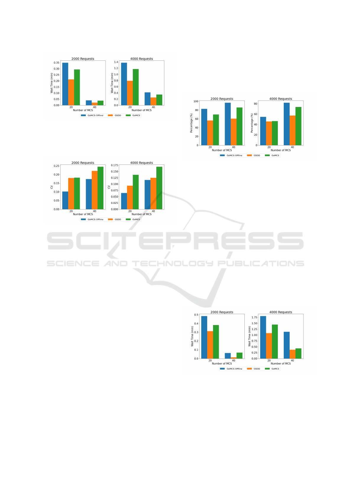
Figure 2: Average Waiting Time of EVs.

the EVs have to wait for free ports to start charging,

which increases the wait time; however this is again

reduced as the number of MCSs increase as expected.

Figure 3: Coefﬁcient of Variance of Requests Served.

Fig. 3 shows the coefﬁcient of variance (CV)

of requests served per MCS with varying number of

MCSs and requests. It is seen that the CV value

decreases with the number of requests and increases

with the number of MCS. This happens because when

there are multiple MCSs and fewer requests in the

same area, some MCSs may remain idle, leading to

a higher CV. GoMCS-Ofﬂine has the least variation,

which is expected as with exact knowledge of future

requests, it can distribute the requests to MCSs more

evenly.

5.2 Scenario 2: Urban Commute

Charging Requests

In this scenario, charging requests are simulated from

EVs traveling in a pattern similar to commuter pat-

terns in a metropolitan city. In the ﬁrst half of the

day, people move from the suburbs (outskirts) to the

central part of the city for jobs, business etc., and the

opposite happens in the second half of the day. While

generating the dataset, the probability of picking up

a location as the starting or ending point is adjusted

according to its distance from the city center. In the

ﬁrst half, the starting point of a request is chosen with

a probability that is directly proportional to its dis-

tance from the city center. Similarly, while picking

the destination, it is taken as inversely proportional to

the distance from the city center. This dataset tries

to represent the charging needs across a typical big

city, where the deployment of MCSs makes the most

sense.

Figure 4: Percentage of requests served.

Fig. 4 shows the percentage of requests served

for varying number of MCSs and requests. It is seen

that as we increase the number of MCSs, the percent-

age of requests served always increases as expected.

The GoMCS algorithm performs much better than

GSDD in this case also. One change to note is that

across most cases, the percentage of served requests

decreases from Scenario 1. This is because the MCSs

are not distributed according to the trafﬁc patterns,

causing variation in use of MCSs.

Fig. 5 shows the average waiting time of an EV

for varying number of MCSs and requests. The trends

are similar to that in Scenario 1, for similar reasons.

The waiting time for all cases increases compared to

Scenario 1 as if the trafﬁc is congested in a speciﬁc

area and a limited number of MCSs are in that area,

then the EVs will need to wait for a longer time. The

trends for the coefﬁcient of variation are also similar

and is not shown separately here again.

Figure 5: Average Waiting Time of EVs.

Dynamic Charging on the Go: Optimizing Mobile Charging Stations for Electric Vehicle Infrastructure

471

5.3 Scenario 3: Repetitive Random

Charging Requests

In this dataset, for the ﬁrst few days, we generate re-

quests from EVs occurring at random locations with

random destinations without any discernible pattern

or correlation between successive requests. Then,

from a particular day onward, the requests lie within

a certain time and distance bound of the requests that

occur on the previous day and thus are similar. A

similarity index (s

) is deﬁned which decides these

bounds on the time and distance, with 0 indicating

that the request pattern is completely random and 1

indicating that the request pattern of consecutive days

are exactly the same. The time and distance bounds

are set as 30 × (1 − s

) minutes and 5000 × (1 − s

)

meters respectively, where s

varies from 0 to 1.

Figure 6: Percentage of requests served.

Fig. 6 shows the percentage of requests served for

different number of MCSs and number of requests.It

is seen that as we increase the number of MCSs, the

percentage of requests served always increases for

the same reason as described earlier. GoMCS per-

forms much better than GSDD in this case also. One

change to note in this case is that although the val-

ues for GoMCS-Ofﬂine remain almost the same, the

performance of both GoMCS abd GSDD algorithms

improves, with GoMCS performing almost as well as

GoMCS-Ofﬂine. This happens as the heuristic is able

to learn from past request patterns effectively.

Fig. 7 shows the average waiting time of EVs for

varying number of MCSs and requests. From Fig. 2

and Fig. 7, it is seen that although the percentage of

requests served increases for GoMCS and GSDD, the

waiting times remain almost the same or decrease in

some cases. This shows that the algorithms are able

to better distribute the MCSs according to the trafﬁc

patterns.

Figure 7: Average Waiting Time of EVs.

Fig. 8 shows the coefﬁcient of variance (CV)

of requests served per MCS. for varying number of

MCSs and requests. The CV of GoMCS and GSDD

are both slightly less compared to Scenario 1, due to

better prediction of demand resulting in more even

distribution.

Figure 8: Coefﬁcient of Variance of Requests Served.

For this scenario, the robustness of GoMCS to

deviations in the recurring spatiotemporal pattern of

requests is also evaluated for 2000 requests and 20

MCSs. GoMCS is run normally for a few days and

then, for a certain day, the request pattern is changed

to different patterns. In the ﬁrst case, the start and end

points of the requests are generated randomly across

the city on each day. In the second case, the re-

quests are generated with the start points being closer

to the city center and the end points being away from

the city center. In the third case, the start points are

chosen away from the city center and the end points

closer to the city center. Table 3 shows the results.

As the MCSs are almost evenly distributed on a nor-

mal day, performance difference for the ﬁrst case is

not signiﬁcant. In the second case, the EVs are near

the center of the city, so the MCSs located in the out-

skirts are underutilized, and those near the center are

overloaded, which reduces the percentage of requests

served. When EVs move from outskirts of the city,

many trips still pass through the center of the city

so the MCSs in the city center are less underutilized;

hence the fall in performance is much less.

VEHITS 2025 - 11th International Conference on Vehicle Technology and Intelligent Transport Systems

472

Table 3: Robustness with Request Patterns.

Request Pattern % Served

Normal day (Recurring) 80.1

Random requests 78.8

Request mainly near city center 74.9

Request mainly from outskirts 77.1

REFERENCES

Atmaja, T. D. and Mirdanies, M. (2015). Electric vehicle

mobile charging station dispatch algorithm. Energy

Procedia, 68:326–335. 2nd International Conference

on Sustainable Energy Engineering and Application

(ICSEEA) 2014.

Cui, S., Zhao, H., and Zhang, C. (2018). Multiple types

of plug-in charging facilities’ location-routing prob-

lem with time windows for mobile charging vehicles.

Sustainability, 10(8).

El-Fedany, I., Kiouach, D., and Alaoui, R. (2021). A smart

coordination system integrates mcs to minimize ev

trip duration and manage the ev charging, mainly at

peak times. International Journal of Intelligent Trans-

portation Systems Research, 19.

Jeon, S. and Choi, D.-H. (2021). Optimal energy manage-

ment framework for truck-mounted mobile charging

stations considering power distribution system oper-

ating conditions. Sensors, 21(8).

Kaggle (2023). Ev charging station usage of california city.

https://www.kaggle.com/ds/3417518.

Kong, P.-Y. (2019). Autonomous robot-like mobile chargers

for electric vehicles at public parking facilities. IEEE

Transactions on Smart Grid, 10(6):5952–5963.

Liu, L., Xi, Z., Zhu, K., Wang, R., and Hossain, E. (2022).

Mobile charging station placements in internet of elec-

tric vehicles: A federated learning approach. IEEE

Transactions on Intelligent Transportation Systems,

23(12):24561–24577.

Liu, Q., Li, J., Sun, X., Wang, J., Ning, Y., Zheng, W.,

Li, J., and Liu, H. (2018). Towards an efﬁcient and

real-time scheduling platform for mobile charging ve-

hicles. In Vaidya, J. and Li, J., editors, Algorithms and

Architectures for Parallel Processing, pages 402–416.

Springer International Publishing.

Moghaddam, V., Ahmad, I., Habibi, D., and Masoum,

M. A. (2021). Dispatch management of portable

charging stations in electric vehicle networks. eTrans-

portation, 8:100112.

OSRM (2024). Open source routing machine.

https://project-osrm.org/.

Raboaca, M.-S., Bancescu, I., Preda, V., and Bizon, N.

(2020). An optimization model for the temporary

locations of mobile charging stations. Mathematics,

8(3).

Tang, P., He, F., Lin, X., and Li, M. (2020). Online-to-

ofﬂine mobile charging system for electric vehicles:

Strategic planning and online operation. Transporta-

tion Research Part D: Transport and Environment,

87:102522.

Wang, F., Chen, R., Miao, L., Yang, P., and Ye, B.

(2019). Location optimization of electric vehicle

mobile charging stations considering multi-period

stochastic user equilibrium. Sustainability, 11(20).

Zhang, X., Cao, Y., Peng, L., Li, J., Ahmad, N., and Yu, S.

(2020). Mobile charging as a service: A reservation-

based approach. IEEE Transactions on Automation

Science and Engineering, 17(4):1976–1988.

Dynamic Charging on the Go: Optimizing Mobile Charging Stations for Electric Vehicle Infrastructure

473