Landmark-Based Geopositioning with Imprecise Map
No
¨
el Nadal
a
, Jean-Marc Lasgouttes
b
and Fawzi Nashashibi
c
Inria, France
Keywords:
Autonomous Navigation, Autonomous Vehicles, Landmark-Based Localization, Fusion and Estimation.
Abstract:
This paper introduces a novel approach for real-time global positioning of vehicles, leveraging coarse
landmark maps with Gaussian position uncertainty. The proposed method addresses the challenge of precise
positioning in complex urban environments, where global navigation satellite system (GNSS) signals alone
do not provide sufficient accuracy. Our approach is to achieve a fusion of Gaussian estimates of the vehicle’s
current position and orientation, based on observations of the vehicle, and information from the landmark
maps. It exploits the Gaussian nature of our data to achieve robust, reliable and efficient positioning, despite
the fact that our knowledge of the landmarks may be imprecise and their distribution on the map uneven. It
does not rely on any particular type of sensor or vehicle. We have evaluated our method through our custom
simulator and verified its effectiveness in obtaining good real-time positional accuracy of the vehicle, even
when the GNSS signal is completely lost, even on the scale of a large urban area.
1 INTRODUCTION
Global positioning or geopositioning (Kumar and
Muhammad, 2023) is one of the fundamental tasks re-
quired for autonomous vehicle navigation. The need
is to be able to obtain a decimeter or even a centimeter
position accuracy, in terms of global accuracy. Satel-
lite signal receivers (GNSS) such as Galileo, GPS,
Glonass or Baidu are widely used for less precise ge-
olocation. However, when it comes to navigation in
urban environments, these solutions suffer from un-
availability and conceptual failures (Bresson et al.,
2017): multiple paths due to urban canyons, unfavor-
able satellite configurations, atmospheric conditions,
etc. On the other hand, solutions based on GNSS RTK
with centimeter accuracy are very expensive.
In order to remedy this, the positioning solutions
envisaged are based on the use of on-board and re-
mote digital maps (Chalvatzaras et al., 2022; Elghaz-
aly et al., 2023). Such maps are assumed to provide
the autonomous vehicle with information, some of
which can be perceived by their sensors and repre-
sented by point clouds (Li et al., 2021), occupancy
grids (Alsayed et al., 2015), or lane graphs (Z
¨
urn
et al., 2021; B
¨
uchner et al., 2023).
a
https://orcid.org/0009-0005-0340-6836
b
https://orcid.org/0000-0001-7507-0378
c
https://orcid.org/0000-0002-4209-1233
Another possibility is to use maps holding geopo-
sitioned local information (or landmarks) (Qu et al.,
2018). These landmarks can be modeled as two-
or three-dimensional points (Stoven-Dubois, 2022;
Zhang et al., 2023) or as more complex geometric
shapes (Ruan et al., 2023), and should be natural fea-
tures (e.g. trees) or artificial features (e.g. poles, road
signs, traffic lights, building corners, road markings)
that are easily recognizable by vehicles on the road. In
order to estimate a geo-referenced position, a vehicle
uses its on-board perception sensors to detect certain
landmarks in the immediate environment, either on its
own (Stoven-Dubois, 2022; Weishaupt et al., 2024)
or collaboratively (Chen et al., 2020), and then pro-
ceeds with matching them with the ones stored in the
map. Naturally, the more vehicles detect landmarks,
the more there will be in the map, which requires per-
formance issues to be tackled as well (Alsayed et al.,
2015). Another challenge is then to keep the land-
marks map robust and accurate (Dissanayake et al.,
2002; Sun et al., 2022; He et al., 2022).
In this paper, we assume that we have at our dis-
posal a map of the urban road environment and an
associated landmark map with Gaussian uncertainty
(the reason for this choice will be explained later).
Each landmark comes with a Gaussian error and we
propose a global positioning method using this impre-
cise information. Here, we are addressing the prob-
474
Nadal, N., Lasgouttes, J.-M. and Nashashibi, F.
Landmark-Based Geopositioning with Imprecise Map.
DOI: 10.5220/0013287300003941
Paper published under CC license (CC BY-NC-ND 4.0)
In Proceedings of the 11th International Conference on Vehicle Technology and Intelligent Transport Systems (VEHITS 2025), pages 474-481
ISBN: 978-989-758-745-0; ISSN: 2184-495X
Proceedings Copyright © 2025 by SCITEPRESS – Science and Technology Publications, Lda.

lem of geopositioning in a city. Landmarks should be
visible and detected with sufficient reliability by the
algorithms at our disposal, despite the specific con-
straints of an urban environment: for instance, the risk
that landmarks can be partially or totally occluded by
surrounding mobile or parked vehicles. The proposed
solution must enable the vehicle to position itself pre-
cisely, and without the help of a GNSS system.
We propose a vehicle geopositioning approach us-
ing landmarks whose precise positions are not neces-
sarily known. This method is effective enough to be
ran in real time, assuming that the vehicle’s speed cor-
responds to what is generally observable in an urban
environment. Based on the sensors’ and the map’s re-
spective accuracy, we are able to determine both the
most likely position of the vehicle and its Gaussian er-
ror. This is not a SLAM (Simultaneous Localization
And Mapping) (Durrant-Whyte and Bailey, 2006) ap-
proach as the construction of the map (which is more
sparse than in most SLAM settings) is handled sepa-
rately, although it influenced the way we defined our
map while working on this approach.
The paper is organized as follows: Section 2 gives
further details regarding our methodology and the
workflow of the method. The experiments performed
on our simulator are then reported and analyzed in
Section 3. Finally, Section 4 outlines future work.
2 METHODOLOGY
2.1 Data Association
We need to associate the perception-based observa-
tions and the landmarks that are already known and
stored in the map. We take into account the covari-
ance between the positions coordinates, in order to
take advantage of the Gaussian model adopted. We
have adopted a GCBB (Geometric-based Compatibil-
ity Branch and Bound) (Neira et al., 2003; Breuel,
2003) algorithm, in order to carry out this type of data
association.
This algorithm attempts to construct a set of pairs,
each consisting of an observation and a landmark, that
satisfy the given compatibility constraints. The search
for the best-fitting such set is performed by incremen-
tally constructing the tree of the solution space, which
allows for efficient search space pruning. Starting
from an empty set, the algorithm proceeds in a depth-
first branch and bound manner. At the leaf level of
the tree, the algorithm checks whether it has come up
with a hypothesis that has a better compatibility score
than the current best one. For this purpose, we con-
sider a unary constraint and a binary constraint.
For the unary constraint, we calculate a compati-
bility score between each observation and each land-
mark. This score depends on both the Euclidean dis-
tance between their positions, and on the covariance
associated with these data. This score is then com-
pared with a threshold, that is set at the beginning of
the experiment, to determine whether or not the as-
sociation is possible, which leads to the unary con-
straint. Formally, let us consider that an observation
is given by a multivariate Gaussian distribution vector
o and a covariance matrix Σ
o
, and a landmark position
by a multivariate Gaussian distribution vector m and
a covariance matrix Σ
m
. We define d = m − o and
Σ
d
= Σ
o
+ Σ
m
. The constraint between this observa-
tion and this landmark is then defined as:
unary(m, o)
def
= d
𝑇
Σ
−1
d
d < 𝜒
2
2, 𝛼
(1)
where 𝜒
2
2, 𝛼
is a 𝜒
2
random variable with two degrees
of freedom, and such that 𝛼 = 0 .95.
While the unary constraint measures the possi-
bility of a match, the binary constraint evaluates the
compatibility between two matches. Given two land-
marks 𝑖 and 𝑗, we denote Σ
m|𝑖 𝑗
the covariance sub-
matrix of Σ
m
using only rows and columns that corre-
spond to 𝑖 and 𝑗. We then define the following.
b
m
𝑖 𝑗
def
= 𝑓
𝑖 𝑗
(m
𝑖
, m
𝑗
) =

𝑚
𝑗 𝑥
− 𝑚
𝑖𝑥
𝑚
𝑗 𝑦
− 𝑚
𝑖𝑦

, (2)
J
m
𝑖
def
=
𝜕 𝑓
𝑖 𝑗
𝜕m
𝑖




(m
𝑖
,m
𝑗
)
, (3)
J
m
𝑗
def
=
𝜕 𝑓
𝑖 𝑗
𝜕m
𝑗




(m
𝑖
,m
𝑗
)
, (4)
P
m
𝑖 𝑗
def
= J
m
𝑖
Σ
m|𝑖 𝑗
J
m
𝑖
𝑇
+ J
m
𝑗
Σ
m|𝑖 𝑗
J
m
𝑗
𝑇
+ J
m
𝑖
Σ
m|𝑖 𝑗
J
m
𝑗
𝑇
+ J
m
𝑗
Σ
m|𝑖 𝑗
J
m
𝑖
𝑇
. (5)
We define similar notations for any two observa-
tions o
𝑙
and o
𝑙
, with covariance matrix Σ
o| 𝑘𝑙
defined
in the same fashion as above.
The binary constraint between the matches
(o
𝑘
, m
𝑖
) and (o
𝑙
, m
𝑗
) is then defined as
binary(o
𝑘
, m
𝑖
, o
𝑙
, m
𝑗
)
def
= (6)
(b
o
𝑘𝑙
− b
m
𝑖 𝑗
)
𝑇
(P
o
𝑘𝑙
+ P
m
𝑖 𝑗
)
−1
(b
o
𝑘𝑙
− b
m
𝑖 𝑗
) < 𝜒
2
2, 𝛼
where again 𝛼 = 0.95.
If more than one possible matches are found, then
the matching score is defined as being the mean of
unary(m, o) and binary(o
𝑖
, m
𝑗
, o
𝑘
, m
𝑙
) values. The
matching with the lowest score is chosen.
In order to optimize its execution time, the algo-
rithm only takes into account landmarks which satisfy
the following property: there is at least one observa-
tion such that the compatibility score between this ob-
servation and the landmarks is below the threshold set
Landmark-Based Geopositioning with Imprecise Map
475

previously. Landmarks that are known to be at a large
distance of the vehicle’s estimated position are dis-
carded beforehand, as they have negligible chance of
being associated to an observation by the algorithm.
Once this data association is performed, ℓ ≤ 𝑚
observations have been matched to an existing land-
mark. For each such observation 𝑖, using the map’s in-
formation regarding the corresponding landmark, we
compute an estimation (𝑥
est
𝑖
, 𝑦
est
𝑖
) of the vehicle’s po-
sition. This leads to a 2ℓ-dimensional Gaussian dis-
tribution vector z, composed of all 𝑥
est
𝑖
followed by
all 𝑦
est
𝑖
.
2.2 Fusion of Gaussian Vectors
Once the data association has been carried out, each
observation provides an estimate of the vehicle’s cur-
rent position, as well as the covariance between these
estimates (which are map data). These estimates are
then merged to determine the most likely vehicle po-
sition, in the form of a Gaussian variable.
In this part, we have 2ℓ measurements (ℓ for each
coordinate), together with the corresponding covari-
ance matrix Σ
ℓ
, and A
ℓ
= Σ
−1
ℓ
the corresponding
precision matrix (both being square matrices of size
2ℓ × 2ℓ). To perform the fusion, we maximize the
probability density of this distribution, by differenti-
ating the associated log-likelihood with respect to the
unknown vehicle position v. A unique maximum is
then found.
Formally, we consider a vector z of estimates of
size 2ℓ, the first ℓ coordinates corresponding to esti-
mates of the x coordinate and the ℓ others to estimates
of the y coordinate. Let, e = (1, . . . , 1)
𝑇
a vector of
size 2ℓ and E of size 2 × 4ℓ defined as
E
def
=

e 0
0 e

. (7)
If the true value measured by the vehicle is v, then
the probability density of our measurements is now
𝑝(z|v) =
1
𝑍
exp

−
1
2
(
Ev − z
)
𝑇
A
ℓ
(
Ev − z
)

, (8)
where 𝑍 is a constant.
We seek to maximize this value by differentiating
the log-likelihood with respect to z, which leads us to
E
𝑇
A
ℓ
Ev − E
𝑇
A
ℓ
z = 0, (9)
which is easily solved to yield the following estima-
tion for the position of the vehicle
v = Mz, with M = (E
𝑇
A
ℓ
E)
−1
E
𝑇
A
ℓ
. (10)
The covariance matrix of v is given by:
Σ
v
= M
𝑇
Σ
ℓ
M (11)
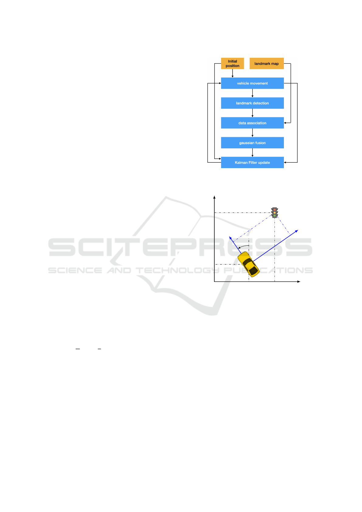
Figure 1: Summary of our approach. The initial position
and the landmark maps are known to the vehicle at the be-
ginning.
𝑥
ℓ
𝑦
ℓ
𝑥
𝑣
𝑦
𝑣
𝑥
𝑜
𝑦
𝑜
𝜃
𝑣
Figure 2: Coordinates of a landmark in global and local
frame of reference.
2.3 Workflow
We assume that the vehicle has local access to a map
with 𝑛 landmarks, whose positions are known up to a
given accuracy. Assuming that the two-dimensional
points describing landmarks follow a multivariate
Gaussian distribution, the map thus represents them
as a 2𝑛-dimensional Gaussian vector, the 𝑛 first coor-
dinates being the 𝑥-coordinates of the landmarks, and
the 𝑛 last coordinates being their 𝑦-coordinates. Let 𝝁
of dimension 2𝑛 be its location, Σ its 2𝑛 × 2𝑛 covari-
ance matrix, and A = Σ
−1
its precision matrix.
Our approach is summarized in Figure 1. Initially,
we assume that our knowledge of the vehicle’s coor-
dinates are accurate up to a centered Gaussian error 𝜖
𝑖
.
The algorithm is run once after each time interval Δ𝑡.
At each iteration, the vehicle is assumed to move on
the map on a straight line, with a speed 𝑣 and an an-
VEHITS 2025 - 11th International Conference on Vehicle Technology and Intelligent Transport Systems
476

gle 𝜃. We apply centered Gaussian errors with stan-
dard deviations 𝜖
𝑣
and 𝜖
𝜃
on these two values, and this
leads to a new estimation of the vehicle’s position.
Then, the vehicle detects 𝑚 ≤ 𝑛 landmarks, ini-
tially not associated to any of the map. We assume
though that the map contains all the landmarks that
could possibly be detected, meaning that any obser-
vation necessarily corresponds to a known landmark.
Each observation corresponds to the position of one of
these landmarks in the vehicle’s frame of reference,
as shown in Figure 2. We take into account the im-
perfection of the sensors used, assuming that they are
correctly calibrated to avoid bias, so that the coordi-
nates of each landmark 𝑙 at time 𝑡 are determined up
to an error that is a centered Gaussian with standard
deviation 𝜖
lmk,𝑙,𝑡
. These coordinates can then be con-
verted into absolute coordinates, which can then be
compared with the coordinates of the map landmarks.
We then perform data association between the
map landmarks and the detected landmarks using the
Geometric Compatibility Branch and Bound (GCBB)
algorithm described in Section 2.1. Each matched ob-
servation leads to an estimation of the vehicle’s cur-
rent position, under the form of a Gaussian vector,
which give us ℓ ≤ 𝑚 such vectors. Right after this data
association we adjust the vehicle’s estimated angle if
this leads to a better score for this specific matching:
we check values above the base estimate with a step
of ΔΘ radians, until the compatibility score no longer
decreases, then do the same for lower values.
These ℓ ≤ 𝑚 vectors are then used to perform a
Gaussian fusion (Section 2.2), that leads to a single
estimation for the vehicle’s position, with the corre-
sponding covariance matrix. Finally, the new vehi-
cle position estimation is obtained through a linear
Kalman Filter (Kalman, 1960), which state space only
contains the vehicle’s coordinates v. The Gaussian fu-
sion estimation, along with the previously estimated
position after the vehicle moved, are used as inputs
to predict and update the vehicle’s coordinates using
results from previous iterations. Then the algorithm
loops with the corrected vehicle position.
3 EXPERIMENTATION
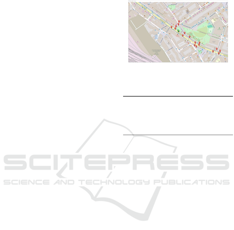
3.1 Simulator
This model was tested using a simulator (see Fig-
ure 3), implemented in C++ using the RTMaps soft-
ware (Nashashibi, 2000). The idea is to have a vehi-
cle move on a local map with a constant speed. This
local map consists in a simplified version of an Open-
StreetMap export of the 12
th
arrondissement of Paris.
Figure 3: Illustration of our simulator. The vehicle (green
marker) geopositions itself thanks to the landmarks (red
markers).
Table 1: Numerical values used for the simulation.
Δ
𝑡
40 ms iteration duration
ΔΘ 0.005 rad angle adjustment step
𝜖
𝑖
0.1 m initial position error
𝜖
𝑚
0.1 m landmark position error (map)
𝜖
𝑣
0.056 m/s vehicle speed error
𝜖
𝜃
0.0044 rad vehicle angle error
We retrieve the information regarding the streets and
their nodes to create an oriented graph on which the
vehicle may move. In addition, we provide a set of
landmarks, which we assume detectable by our simu-
lated vehicle. Such landmarks would correspond in
reality to those detectable by vehicles with current
technology, some of which were listed in Section 1.
Given that these landmarks’ coordinates are a priori
accurate, and in order to simulate the fact that the
landmarks of the actual map will not be accurate, a
centered Gaussian error with a standard deviation of
𝜖
𝑚
is assigned to each coordinate. In this way, the ve-
hicle will detect landmarks at positions that are close
yet different from the ones that are stored in the map
that the vehicle uses to position itself. Even though
our method relies on the GCBB algorithm, the fact
that the landmarks in the map are not correlated im-
plies that the binary constraint of this algorithm is use-
less in this particular simulation setup. In Section 4
we will go back to this point in order to explain how
we intend to build a map with covariance.
The simulator simultaneously determines two po-
sitions: the vehicle’s actual position (where it re-
ally is), and the vehicle’s perceived position (where it
thinks it is). Each time the vehicle moves, the actual
movement and the landmark detection are returned
with additional error, using the numerical values in
Table 1. For the sake of the experimentation, the ve-
hicle moves at a constant speed of 30 km/h.
In these experiments we also tried to simulate the
fact that, in real life, certain landmarks are likely to
Landmark-Based Geopositioning with Imprecise Map
477

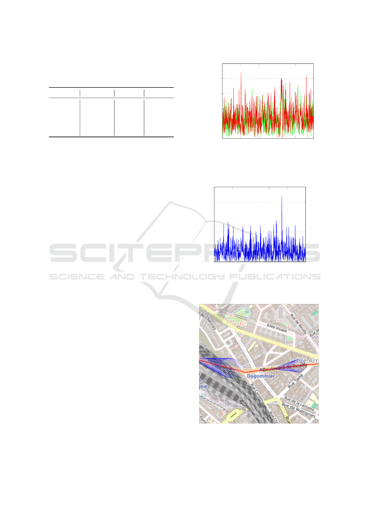
Table 2: Cumulative distribution of the geopositioning er-
rors depending on the landmark density. For example, with
an average of 1 landmark per 10.5m, about 81.2% of the
position estimates have an error of less than 0.1m.
Error (m) 1 p. 10.5m 1 p. 14m 1 p. 21m
< .05 35.2% 35.5% 30.8%
< .1 81.2% 80.8% 75.4%
< .15 96.8% 96.6% 94.2%
< .2 99.6% 99.5% 98.6%
< .4 100% 100% 100%
be hidden (for example, by another vehicle, construc-
tion work, buildings. . . ). To this end, at each iteration
every landmark that is currently visible has a 0.001
probability to become hidden for a given number of
iterations ranging between 1 (40 ms) and 1000 (40 s),
following a uniform law.
For simplicity, we assume that only landmarks
that are less than 50 m away from the vehicle are pos-
sibly visible, regardless of the location and shape of
nearby buildings. Finally, for performance purposes,
we limit the number of landmarks that can be detected
at a given moment to 5: if there are more than 5 vis-
ible landmarks at some point then the 5 landmarks
with the largest estimated distance to the vehicle are
selected. Indeed, in practice, more distant landmarks
yield a better vehicle angle estimation.
The hardware used in practice inevitably has an
impact on the performance of this approach. For in-
stance, the measured errors will necessarily depend
on the type of sensor used to detect the landmarks,
such as cameras, radars, or LiDARs. However, most
of these technical details are modeled in this paper by
the correlation matrix, in Gaussian form. For exam-
ple, irrespective of the sensors used, it is assumed that
the detection of a landmark by a vehicle is represented
by the estimated coordinates of the landmark together
with the corresponding error. Similarly, the issues
surrounding vehicle-server communications are not
studied. Hence, our method does not rely on a spe-
cific type of sensor and may be used without the need
of taking specific technical constraints into account.
As one of our goals is to provide an effective geoposi-
tioning without the use of expensive sensors, we have
deliberately used mediocre values for the mean er-
ror estimations to make sure that the results that we
obtain are still acceptable despite this additional con-
straint and degraded operational conditions.
3.2 Results
The numerical results presented here correspond to a
1 h simulated ride, using a map which contains land-
marks that were generated for the sake of the ex-
10 11 12 13 14
15
0
0.05
0.1
0.15
0.2
0.25
Traveled distance (km)
Error (m)
Figure 4: Evolution of the positioning error for the fusion
estimation (green) and on the Kalman filter estimation (red)
between kilometer 10 and kilometer 15 (restricted for clar-
ity). Average landmark density is one every 21 m.
10 11 12 13 14
15
0
0.01
0.02
Traveled distance (km)
Error (rad)
Figure 5: Evolution of the error on vehicle’s angle estima-
tion between kilometer 10 and kilometer 15 (restricted for
clarity). Average landmark density is one every 21 m.
Figure 6: Evolution of the position estimation standard de-
viation (in blue) on a short portion of the simulation (not
to scale, maximum standard deviation is slightly less than
15 cm in practice). The vehicle’s trajectory is in red.
VEHITS 2025 - 11th International Conference on Vehicle Technology and Intelligent Transport Systems
478

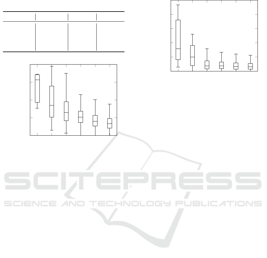
Table 3: Cumulative distribution of the angle errors depend-
ing on the landmark density.
Error (rad) 1 p. 10.5m 1 p. 14m 1 p. 21m
< .005 71.7% 71.9% 70.8%
< .01 96.9% 96.8% 96.1%
< .015 99.9% 99.9% 99.7%
< .05 100% 100% 100%
0 1 2 3 4 5
0
0.1
0.2
0.3
0.4
Number of detected landmarks
Error (m)
Figure 7: Boxplots (median/quartiles/1.5*IQR) of the
geopositioning error of the Kalman filter’s estimation, con-
ditionally on the number of detected landmarks. Average
landmark density is one every 21 m.
periment. In order to explore the impact of varying
landmark densities in the urban environment, each
of these experiments features a different number of
known landmarks on the map. These landmarks are
generated randomly, with an algorithm that ensures
that they are sufficiently close to the roads on which
the vehicle is likely to travel. The maps that have
been produced for this experiment contain respec-
tively 2000, 3000 and 4000 landmarks. If we assume
that all these landmarks are supposed to be on the side
of a road, we can translate this into the average num-
ber of meters of road per landmark: respectively one
landmark per 10.5 m, 14 m and 21 m. Another way to
describe it is that landmark densities are respectively
2185, 1639 and 1092 per square kilometer, based on
the area exported from OpenStreetMap.
Table 2 and Table 3 respectively show the distri-
bution of the vehicle’s position and angle errors val-
ues. Except for these two tables, the results reported
in this section correspond to the less dense landmark
map, with 2000 items.
Figure 4 and Figure 5 respectively show the evo-
lution of the distance between the vehicle’s estimated
coordinates and the real coordinates and the absolute
difference between the vehicle’s estimated headway
and the real angle during the 1 h long runs.
Figure 6 shows the evolution of the standard de-
0 1 2 3 4 5
0
0.01
0.02
0.03
0.04
0.05
Number of detected landmarks
Error (rad)
Figure 8: Boxplots (median/quartiles/1.5*IQR) of the angle
error of the Kalman filter’s estimation, conditionally on the
number of detected landmarks. Average landmark density
is one every 21 m.
viation of the position estimation on a short portion
of the simulation. We can see that the standard de-
viation increases gradually until a landmark is found,
then stays very low until no landmark is found any-
more.
Figure 7 shows the evolution of accuracy as a
function of the number of landmarks the vehicle de-
tects and matches to the map landmarks. Figure 8
describes the angle estimation error, again depending
on the number of landmarks the vehicle detects and
matches to the map landmarks.
3.3 Analysis
In terms of performance, each iteration of the algo-
rithm runs in less than 40 ms, which means that our
method can be used in real time. As expected, the data
association part of the algorithm is the most CPU-
consuming part, and taking into account more than
5 landmarks at once could cause the running time to
grow drastically. the other CPU-intensive step in the
algorithm is the initialization of the data association,
which takes place in linear time in the number of land-
marks in the map, which can increase significantly
as we scale up the map size. Although this is not
a primary focus of this paper, robust solutions exist
to handle large urban environments, such as in (Al-
sayed et al., 2015), and can be easily integrated into
our current work. Gaussian estimation fusion per-
forms a number of matrix inversions and multiplica-
tions bounded by a constant, and the size of the matri-
ces is the number of estimates resulting from the pre-
vious data association (which is less than 5), so this
will never be a performance issue.
Regarding the vehicle’s position and angle estima-
tion error: while the results using 3000 (1 p. 14 m)
Landmark-Based Geopositioning with Imprecise Map
479

and 4000 (1 p. 10.5 m) landmarks were very simi-
lar, it seems that switching from 2000 (1 p. 21 m) to
3000 improves the results a little bit. Despite these
differences, we can see that our goal of keeping the
distance error below 10 cm is achieved at least 96%
of the time.
While this error stays below 0.15 m most of the
time, we notice that it occasionally spikes. A deeper
analysis of the data reveals that this happen in a few
specific areas of the map the vehicle drives in.
As expected, errors are likely to increase in areas
where the number of detected landmarks is low. For
example, when the vehicle detects only one landmark,
the error on the vehicle’s position is highly dependent
on the error on the single detected landmark. This is
likely to occur when the concentration of landmarks is
too low: in practice, for example, traffic lights tend to
be grouped around major junctions, while bus stops
are more isolated from each other. Even when the
vehicle is travelling through an area with a satisfac-
tory number of landmarks, it may happen that some
or all of these landmarks are temporarily hidden, so
that position accuracy may deteriorate for a short time
in such an area. In these experiments, the vehicle de-
tected 3 or more landmarks at least 98% of the time.
In our experimental setting, decimeter accuracy is
unlikely to be achieved consistently if there are not al-
ways enough landmarks visible at the same time. The
question then arises as to how to make the most of the
urban environment to keep the number of landmarks
detectable by a moving vehicle to a maximum.
Regarding the impact of the number of landmarks
observed at once by the vehicle, although the results
for 0 landmark are not necessarily very representative,
given the rarity of such a situation, we can neverthe-
less see that, as expected, the results improve with the
number of matches with known landmarks from the
map. In the specific case of the vehicle’s angle’s esti-
mation, two landmarks seem to be already enough to
significantly improve the estimation’s accuracy.
Although this is rare, we have observed that the
error can occasionally be significant even with a large
number of landmarks observed and associated with
the map. First of all, it should be noted that, as the
number of detected landmarks increases, it generally
takes a few iterations for the error to converge to a
more satisfactory value, which explains why there can
still be significant errors for 1 or more landmarks de-
tected (this also explains why there can be very small
errors for 0 or 1 landmarks detected, which is not a
major issue since we are interested in the maximum
error). Another explanation is that when the number
of landmarks observed is large, the density of land-
marks in the area through which the vehicle is pass-
ing may be higher than average. This implies that
some landmarks are very close to each other, lead-
ing to more frequent association errors than usual, and
therefore to more position estimation errors.
We also investigated the question of whether the
data association errors may have a significant im-
pact on our method’s accuracy. Generally speak-
ing, matching errors involved landmarks that were
generated very close to each other. Therefore, such
wrong matches have a very minor impact on the ve-
hicle’s position estimation and alone do not compro-
mise the goal of decimetric precision. Furthermore,
some common practical methods to improve the data
association, such as defining the landmarks’ orienta-
tion, type (e.g. traffic sign vs. traffic light) or height
have not been used in this simulator, which leave a
lot of room for improvement in the event the accuracy
of this data association algorithm becomes a critical
issue.
Regarding the fact that we only consider at most
5 landmarks at once: in practice, it does not seem
like increasing this threshold significantly improves
the results when using the aforementioned numerical
values. However, since the target is generally to have
a decimeter or better precision, it may be necessary
to increase that threshold when the map is too inaccu-
rate. Future work could include the study of some of
the hyperparameters of this simulation in order to un-
derstand more precisely how, for example, depending
on the accuracy of the map, to find a compromise be-
tween the performance of the algorithm and the num-
ber of observations used to estimate the vehicle’s po-
sition.
4 CONCLUSION
This paper shows how an imprecise landmark map
can contribute in geopositioning an autonomous ve-
hicle. The results obtained using our simulator show
that, depending on the accuracy of the landmark map
and the landmark density, the error in the vehicle’s
coordinates is small enough to replace a GNSS ser-
vice in urban scenarios where such data is unreliable
or unavailable.
We plan to test our method on data collected from
a real vehicle in the near future: this will be facilitated
by the use of the RTMaps software, which allows real
data to be easily collected. One of the challenges will
be to identify families of landmarks that are conve-
nient to detect in an urban setting and dense enough
for our needs.
For the purposes of this work, we have assumed
that we are in possession of a map based on real land-
VEHITS 2025 - 11th International Conference on Vehicle Technology and Intelligent Transport Systems
480

marks that can be detected in practice using exist-
ing technology, but the imprecision of the position
of these landmarks has been artificially defined. In
the longer term, our goal is to use the measurements
made by individual vehicles as crowd-sourced data
for improving the map. In such a system, the vehicles
send all the data that they obtained during a day to a
central server that will consolidate and process them
in order to produce a new landmarks map that will
be sent back to all vehicles. The goal is to improve
on the work of (Stoven-Dubois, 2022) to handle city-
scale maps. Eventually, this will lead to a methodol-
ogy for the creation of precise landmark maps from
coarse ones without resorting to expensive solutions
like GNSS RTK.
REFERENCES
Alsayed, Z., Bresson, G., Nashashibi, F., and Verroust-
Blondet, A. (2015). PML-SLAM: a solution for local-
ization in large-scale urban environments. In PPNIV-
IROS 2015.
Bresson, G., Alsayed, Z., Yu, L., and Glaser, S. (2017).
Simultaneous localization and mapping: A survey of
current trends in autonomous driving. IEEE Transac-
tions on Intelligent Vehicles, 2(3):194–220.
Breuel, T. M. (2003). Implementation techniques for geo-
metric branch-and-bound matching methods. Com-
puter Vision and Image Understanding, 90(3):258–
294.
B
¨
uchner, M., Z
¨
urn, J., Todoran, I.-G., Valada, A., and
Burgard, W. (2023). Learning and aggregating lane
graphs for urban automated driving. In Proceedings
of the IEEE/CVF Conference on Computer Vision and
Pattern Recognition, pages 13415–13424.
Chalvatzaras, A., Pratikakis, I., and Amanatiadis, A. A.
(2022). A survey on map-based localization tech-
niques for autonomous vehicles. IEEE Transactions
on intelligent vehicles, 8(2):1574–1596.
Chen, S., Zhang, N., and Sun, H. (2020). Collaborative lo-
calization based on traffic landmarks for autonomous
driving. In 2020 IEEE International Symposium on
Circuits and Systems (ISCAS), pages 1–5. IEEE.
Dissanayake, G., Williams, S. B., Durrant-Whyte, H., and
Bailey, T. (2002). Map management for efficient si-
multaneous localization and mapping (SLAM). Au-
tonomous Robots, 12:267–286.
Durrant-Whyte, H. and Bailey, T. (2006). Simultaneous lo-
calization and mapping: part I. IEEE robotics & au-
tomation magazine, 13(2):99–110.
Elghazaly, G., Frank, R., Harvey, S., and Safko, S. (2023).
High-definition maps: Comprehensive survey, chal-
lenges and future perspectives. IEEE Open Journal
of Intelligent Transportation Systems.
He, L., Jiang, S., Liang, X., Wang, N., and Song, S.
(2022). Diff-net: Image feature difference based high-
definition map change detection for autonomous driv-
ing. In 2022 International Conference on Robotics
and Automation (ICRA), pages 2635–2641. IEEE.
Kalman, R. E. (1960). A new approach to linear filtering
and prediction problems. Journal of Basic Engineer-
ing, 82(1):35–45.
Kumar, D. and Muhammad, N. (2023). A survey on local-
ization for autonomous vehicles. IEEE Access.
Li, L., Wang, R., and Zhang, X. (2021). A tutorial review
on point cloud registrations: principle, classification,
comparison, and technology challenges. Mathemati-
cal Problems in Engineering, 2021(1):9953910.
Nashashibi, F. (2000).
𝑅𝑇
𝑚𝑎 𝑝𝑠: a framework for proto-
typing automotive multi-sensor applications. In IEEE
Proceedings of the IEEE Intelligent Vehicles Sympo-
sium 2000, pages 99–103. IEEE.
Neira, J., Tard
´
os, J. D., and Castellanos, J. A. (2003). Lin-
ear time vehicle relocation in SLAM. In ICRA, pages
427–433.
Qu, X., Soheilian, B., and Paparoditis, N. (2018). Landmark
based localization in urban environment. ISPRS Jour-
nal of Photogrammetry and Remote Sensing, 140:90–
103.
Ruan, J., Li, B., Wang, Y., and Sun, Y. (2023). Slamesh:
Real-time lidar simultaneous localization and mesh-
ing. In 2023 IEEE International Conference on
Robotics and Automation (ICRA), pages 3546–3552.
IEEE.
Stoven-Dubois, A. (2022). Robust Crowdsourced Mapping
for Landmarks-based Vehicle Localization. PhD the-
sis, Universit
´
e Clermont Auvergne.
Sun, S., Jelfs, B., Ghorbani, K., Matthews, G., and Gilliam,
C. (2022). Landmark management in the application
of radar SLAM. In 2022 Asia-Pacific Signal and In-
formation Processing Association Annual Summit and
Conference (APSIPA ASC), pages 903–910. IEEE.
Weishaupt, F., Tilly, J. F., Appenrodt, N., Fischer, P., Dick-
mann, J., and Heberling, D. (2024). Landmark-based
vehicle self-localization using automotive polarimet-
ric radars. IEEE Transactions on Intelligent Trans-
portation Systems.
Zhang, Y., Severinsen, O. A., Leonard, J. J., Carlone,
L., and Khosoussi, K. (2023). Data-association-
free landmark-based SLAM. In 2023 IEEE In-
ternational Conference on Robotics and Automation
(ICRA), pages 8349–8355. IEEE.
Z
¨
urn, J., Vertens, J., and Burgard, W. (2021). Lane graph
estimation for scene understanding in urban driving.
IEEE Robotics and Automation Letters, 6(4):8615–
8622.
Landmark-Based Geopositioning with Imprecise Map
481