Towards the Automated Selection of ML Models for Time-Series Data
Forecasting
Yi Chen
a
and Verena Kantere
School of Electrical Engineering and Computer Science, University of Ottawa, Ottawa, Canada
Keywords:
Model Selection, Deep Learning, Time-Series Data.
Abstract:
Analyzing and forecasting time-series data is challenging since the latter always comes with characteristics,
such as seasonality, which may impact models’ performance but are frequently unknown before implementing
models. At the same time, the abundance of ML models makes it difficult to select a suitable model for
a specific dataset. To solve this problem, research is currently exploring the creation of automated model
selection techniques. However, the characteristics of the datasets have yet to be considered. Toward this goal,
this work aims to explore the appropriateness of models concerning the features of time-series datasets. We
collect a wide range of models and time-series datasets and choose some of them to conduct experiments to
explore how different elements affect the performances of selected models. Based on the results, we formulate
several outcomes that are helpful in time-series data forecasting. Further, we design a decision tree based on
these outcomes, which can be used as a first step toward creating an automated model-selection technique for
time-series forecasting.
1 INTRODUCTION
Data is recorded and stored over time in a wide range
of domains. These observations lead to a collection
of organized statistics called time-series data, a set of
data points ordered in time (Esling and Agon, 2012;
Peixeiro, 2022). Time-series data analysis and fore-
casting are significant for many applications in busi-
ness and industry, such as the stock market and ex-
change, weather forecasting, and electricity manage-
ment (Mahalakshmi et al., 2016).
The analysis of time series has inherent complex-
ity: 1. Most time series exhibit seasonality or elab-
orate cyclical patterns. 2. Time-series data is often
affected by external factors that should be considered
during analysis. 3. The forecasting of time-series data
usually relies on previous time points, so it is sensi-
tive to variation in time. For these reasons, analyz-
ing and forecasting time-series data has become vi-
tal but challenging. Nevertheless, several methods for
time-series data analysis have been proposed, such as
Autoregressive Integrated Moving Average(ARIMA)
(Box and Tiao, 1975), Prophet (Schuster and Paliwal,
1997), as well as Deep Learning (DL) models.
To perform forecasting with ML models, it is nec-
essary to implement a model appropriate for the char-
a
https://orcid.org/0009-0003-9868-4286
acteristics of the input datasets. However, this is
a challenging task since there is a wide variety of
ML models to choose from and users may not know
the characteristics of the input time-series dataset.
Thus, selecting the appropriate model can be time-
consuming or even inaccurate.
Proposed Solution. To solve the problem of model
selection for time-series data forecasting, we explore
the association of the suitability of models with the
characteristics of input time-series datasets, which
can lead to the design of techniques to select the ap-
propriate model in an automated manner, given an es-
timation of the characteristics of the time-series data.
Toward this end, we have designed a series of exper-
iments that consider various models used for time-
series data forecasting and have selected the most ap-
propriate one based on the characteristics of the input
datasets. Our exploratory experimental analysis leads
to the formation of specific outcomes that can be used
as guidelines for the appropriate selection of models.
In the rest of this paper, Section 2 summarizes re-
lated work and Section 3 gives an overview of our
methodology for creating our exploratory experimen-
tal study. Section 4 describes the evaluation of the
ML/DL models, and Section 5 presents the imple-
mentation of the models. Section 6 presents the ex-
perimental results, and Section 7 describes the pro-
Chen, Y. and Kantere, V.
Towards the Automated Selection of ML Models for Time-Series Data Forecasting.
DOI: 10.5220/0013296100003929
Paper published under CC license (CC BY-NC-ND 4.0)
In Proceedings of the 27th International Conference on Enterprise Information Systems (ICEIS 2025) - Volume 1, pages 813-819
ISBN: 978-989-758-749-8; ISSN: 2184-4992
Proceedings Copyright © 2025 by SCITEPRESS – Science and Technology Publications, Lda.
813

posed outcomes and discusses their possible applica-
tion, showcasing it in the design of a decision tree.
Section 8 concludes the paper and discusses the di-
rection for future work.
2 RELATED WORK
Automated model selection is a topic in ML re-
search that has attracted much interest.In 1994, Yumi
Iwasaki and Alon Y. Levy proposed an algorithm
for selecting model fragments automatically for sim-
ulation (Iwasaki and Levy, 1994). They designed
the algorithm based on relevance reasoning, which is
used to determine which phenomenon can affect the
query (Iwasaki and Levy, 1994). In 2010, Vincent
Calcagno designed and implemented an R package
glmulti to select generalized linear models automat-
ically (Calcagno and de Mazancourt, 2010). In 2016,
Gustavo Malkomes et al. employed Bayesian opti-
mization for automated model selection (Malkomes
et al., 2016). They constructed a novel kernel be-
tween models to explain a given dataset (Malkomes
et al., 2016). Lars Kotthoff et al. released the source
of Auto-WEKA, the addition of automatic selection
technology to the original platform (Kotthoff et al.,
2017). They used the Bayesian optimization method
to help users identify the best approach for their par-
ticular datasets. In recent years, Abdelhak Bentaleb
et al. proposed a kind of Automated Model selection
technique, which is used for predicting network band-
width (Bentaleb et al., 2020).
The automated model selection technique is also
a valuable topic in the time-series data area. In
2020, Yuanxiangyin et al. presented an automated
model selection framework to find the most suitable
model for time series anomaly detection by invoking
a pre-trained model selector and a parameter estima-
tor (Ying et al., 2020). In 2022, Chunnan Wang et
al. proposed an algorithm, AutoTS, which is used
for designing a suitable forecasting model for the
given time-series dataset. They constructed a search
space at first, then employed a two-stage pruning
and a knowledge graph analysis method (Wang et al.,
2022). In 2023, Shehan Saleem and Sapna Kumara-
pathirage created a framework for automated model
selection in natural language processing (Saleem and
Kumarapathirage, 2023). They conducted trials on
two models (BOWRF and FastText) to select the best-
performing models and evaluated the performance by
F1 macro and time (Saleem and Kumarapathirage,
2023). Amazon Web Services released AutoGluton-
TimeSeries, which is a part of AutoGluton framework
(Shchur et al., 2023). It combines classic statistic and
deep learning models with an ensembling technique
and helps users achieve time-series forecasting more
efficiently and simply.
Although several automated model selection tech-
niques have been proposed, most target various areas,
not specifically time-series data. Furthermore, those
techniques that focus on time-series data do not con-
sider the characteristics of time-series datasets, and
they only train the models without this information.
In this work, we fill this gap by conducting experi-
ments and acquiring several outcomes that can be ap-
plied to time-series data forecasting.
3 METHODOLOGY OF
EXPERIMENTS
To extract valuable outcomes for designing an auto-
mated model-selection technique for time-series fore-
casting, we devised a four-step methodology: review
of models, collection and review of datasets, selec-
tion of models and datasets, conduct experiments and
analyze results.
In the following, we give details about the first
three steps of our methodology. The rest of the steps
are summarized in the following sections.
• Review of Models. Various models can be used
for time-series data forecasting. The Autore-
gressive and Moving Average (ARMA) model
is a meaningful way to study time series (Mon-
dal et al., 2014). Based on this, the ARIMA,
one of the most popular algorithms in time-series
data prediction, was proposed (Box and Tiao,
1975).Besides, DL models are available for time-
series data forecasting as well, such as LSTM,
GRU, and Convolutional Neural Network (CNN).
There are also some variations of these models,
like Bidirectional LSTM, Bidirectional GRU, and
CNN LSTM, which are an upgrade of traditional
ones.
• Collection and Review of Datasets. Beyond the
models, we considered the possible characteris-
tics of time-series datasets, especially those time-
series-specific characteristics. A prevalent one
is related to whether the dataset is stationary or
not. Also, time-series datasets may exhibit sea-
sonality. After a thorough search, we obtained
six complete time-series datasets: AEP hourly
(Robikscube, 2023), Air Passengers (Peixeiro,
2022), Steel industry data (csafrit2, 2023), Cana-
dian climate history (bmonikraj, 2023), micro-
data (Peixeiro, 2022), and DailyDelhiClimate
(sumanthvrao, 2023).
ICEIS 2025 - 27th International Conference on Enterprise Information Systems
814

• Selection of Models and Datasets. Then, it
comes to choose some models and datasets to con-
duct an experimental evaluation. We chose sev-
eral types of DL models as these can be effective
for processing non-stationary data. We considered
three categories of such models based on their ar-
chitectures: standard DL networks, bidirectional
networks, and hybrid networks. Due to their ar-
chitectural differences, these categories can have
a complementary performance on various time-
series data. Concerning standard DL networks,
we selected LSTM and GRU. LSTM is a pow-
erful tool for tasks with long-term dependencies,
which is suitable for time-series data. GRU is a
modification of LSTM but with a more straight-
forward structure. Furthermore, we selected the
corresponding bidirectional networks of these two
models to make a 1-1 comparison of their perfor-
mance. Finally, CNN-LSTM represents the hy-
brid neural networks category. CNN-LSTM is one
of the most popular hybrid networks since it com-
bines the capabilities of CNN for spatial feature
extraction and LSTM for processing time-series
data. Besides models, we also selected two of
the six datasets we explored. Since we focus on
time-series datasets, we needed the datasets to ex-
hibit the basic and most important characteristics
of time-series datasets, i.e. stationarity and sea-
sonality. After conducting the ADF Test (Test of
stationarity) (Peixeiro, 2022) and decomposition
on all datasets, we chose DailyDelhaClimate and
Steel industry data. Moreover, these two datasets
are most appropriate because they involve climate
and energy consumption data, which may be af-
fected by external factors.
4 DESIGN OF THE MODEL
EVALUATION
In this section, we describe the datasets and the met-
rics we used in our experimental evaluation, as well
as the design of the experiments.
4.1 Dataset
We have conducted experiments using two datasets
with different characteristics: Steel industry data and
DailyDelhiClimateTrain. Steel industry data is a
dataset about the energy consumption in the steel in-
dustry. This dataset is sourced from the UCI Machine
Learning Repository (csafrit2, 2023).
The DailyDelhiClimateTrain dataset provides
users with the Delhi climate from January 1st, 2013,
to April 24th, 2017. This dataset is collected from
Weather Underground API (sumanthvrao, 2023). The
climate data in a city is a bit regular each year, and its
seasonal composition in STL also indicates it is sea-
sonal.
4.2 Metrics
In our study, we used metrics to evaluate the models in
terms of two aspects: time and accuracy. We use two
metrics of accuracy: the Mean Absolute Percentage
Error (MAPE) and the Mean Squared Error (MSE).
They are employed in both the training and the test
phases to measure the accuracy of the results and help
us understand the suitability of models for the input
datasets.
Beyond these two metrics, we also measured the
epochs in each training process of models, which is a
measurement of processing time.
4.3 Design of Experiments
For our evaluation, we implemented five kinds of neu-
ral network models. These models are used to process
datasets in eight types of phenomena to analyze if dif-
ferent horizons and numbers of features will affect the
performance of the models. Table 1 shows eight ex-
periments with each model.
Table 1: Experiments in Each Model.
Models Experiments
LSTM 1 feature + horizon (1)
Bi-LSTM 1 external feature + horizon (5)
GRU 1 external feature + date features + horizon (1)
Bi-GRU 1 external feature + date features + horizon (5)
CNN-LSTM 2 external features + horizon (1)
2 external features + horizon (5)
2 external features + date features + horizon (1)
2 external features + date features + horizon (5)
In Table 1, the ‘horizon’ is the length of time for
which forecasts are generated. Another factor we con-
sider is the ‘date’ feature, which encapsulates the date
and time of the data collection. For example, elec-
tricity consumption may present some kinds of sea-
sonality and has higher values in summer and lower
values in spring. Moreover, employing ‘external fea-
tures’ while training the model may positively impact
the prediction. For instance, in a factory, energy con-
sumption may result in a change of temperature in-
side, so the data on temperature contributes to the pre-
diction of the amount of energy. Therefore, our exper-
iments also consider either 1 or 2 ‘external features.’
The eight types of experiments are implemented for
each of the five models shown in Table 1. In the fol-
lowing description, these eight kinds of experimental
setups are represented by EXP.1 to EXP.8.
Towards the Automated Selection of ML Models for Time-Series Data Forecasting
815

5 DESCRIPTION OF MODEL
IMPLEMENTATION
In the following, we give details of the implementa-
tion of the models, focusing on scaling and inversing,
as well as windowing.
5.1 Scaling and Inversing
Feature scaling, known as data normalization, is
generally performed during the data preprocessing
step (dotdata, 2024). Scaling the data can help to bal-
ance the impact of all variables on the distance calcu-
lation and can help to improve the performance of the
algorithm (atoti, 2024). In this work, we choose the
MinMaxScaler to normalize the data. Implementating
MinMaxScaler is simple since there is a MinMaxS-
caler class in the preprocessing class of the Sklearn
library that can be imported directly. What we should
only do is fit the data we want to scale on the scaler
and then define the boundary of scaling. After nor-
malization, it is necessary to convert the scaled data
back to the original data range for subsequent analy-
sis and interpretation. This process is called inversing,
and it usually happens after predicting and before the
evaluation of the model.
5.2 Window
Applying DL for forecasting relies on creating appro-
priate time windows, allowing us to correctly format
the data to be fed to neural network models. Data
windowing is a process in which users define a se-
quence of time-series data and separate them into two
parts: inputs and labels (Peixeiro, 2022). In this work,
a function of create_dataset is defined to achieve
this. The create_dataset function receives two pa-
rameters: dataset and look_back. The dataset is the
input dataset that users want to feed to the model
and do the forecasting, and look_back means a ret-
rospective period which indicates the number of pre-
vious points in time used to predict the next point.
At the beginning of the function, it initializes two
lists: dataX and dataY. DataX is used to store the
input features, while dataY stores the correspond-
ing target values. Then, it will come to a loop that
aims to traverse the whole dataset. However, it is
needed for the number of look_back time points to
complete the prediction so that the loop will end un-
til len(dataset) - look_back. Then one line of
a = dataset[i : i + look_back] is used for ex-
tracting the look_back time points starting from in-
dex i from the dataset, and these data will be pro-
cessed for the next value predicting. Then the feature
data a will be added to dataX by append, while the
data at the point in time immediately after look_back
time point is a target which should be added to dataY.
In the end, the two lists initialized at the beginning
will be returned as output.
6 EXPERIMENTAL RESULTS
We present our experimental results for the two se-
lected datasets, namely the DailyDelhaClimate and
the Steel Industry datasets.
6.1 Results of DailyDelhaClimate
Dataset
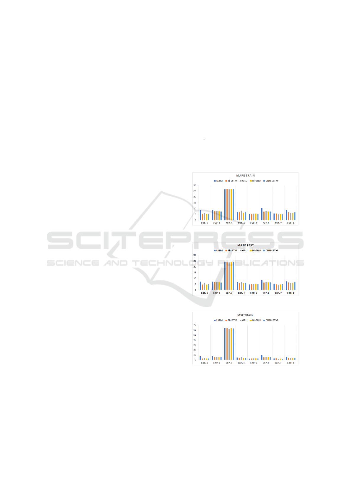
Figure 1: MAPE Train of DailyDelhiClimateTrain.
Figure 2: MAPE Test of DailyDelhiClimateTrain.
Figure 3: MSE Train of DailyDelhiClimateTrain.
The results of the first dataset, DailyDelhaCli-
mate, are shown from Fig.1 to Fig.5. Five metrics:
MAPE Train, MAPE Test, MSE Train, MSE Test,
and epoch are shown separately. The more accurate
model is BiGRU, which achieves the lowest error rate
in experiments 1, 4, and 8, and there are more low er-
ror rates in BiGRU. In contrast, LSTM is less precise
ICEIS 2025 - 27th International Conference on Enterprise Information Systems
816

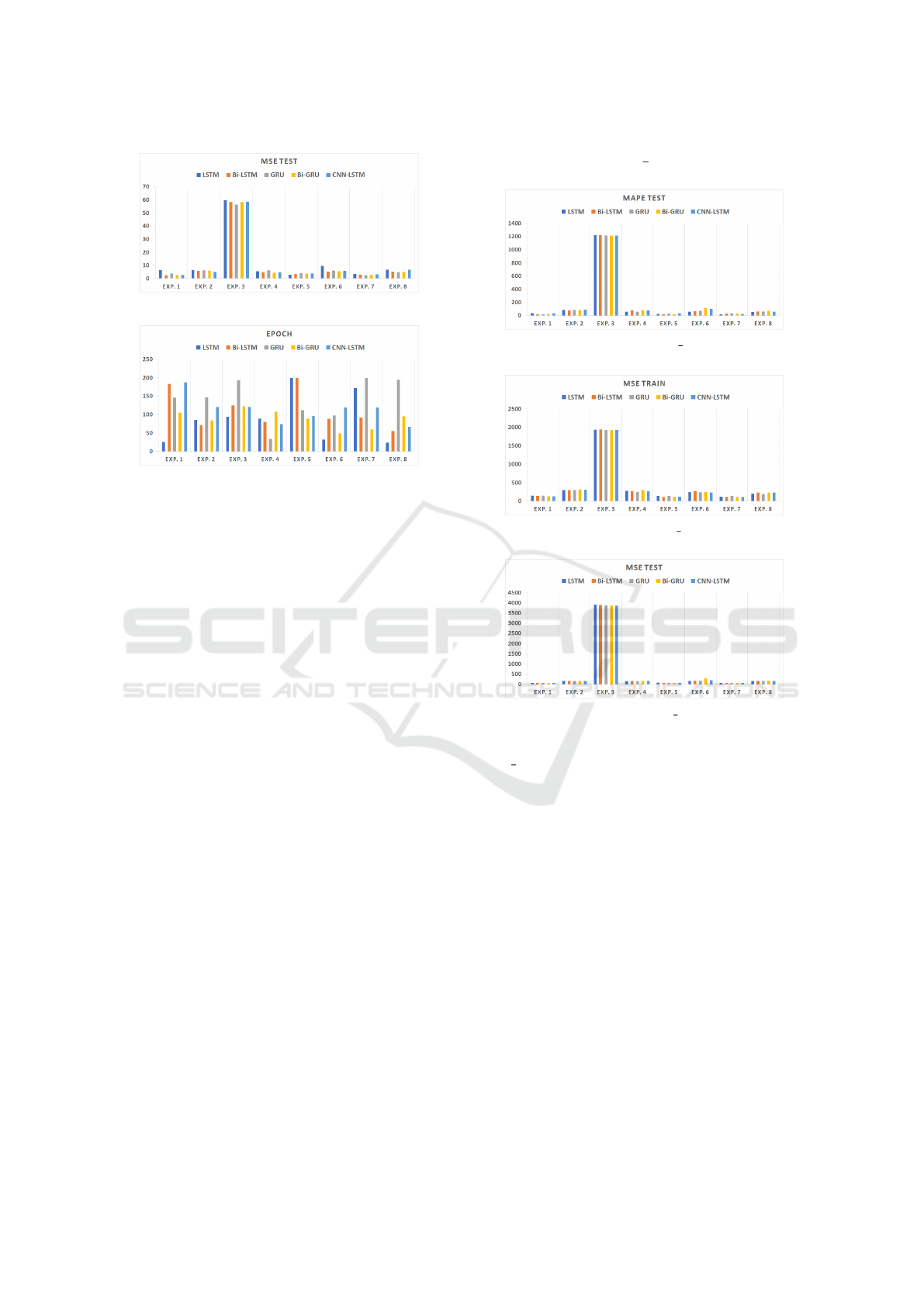
Figure 4: MSE Test of DailyDelhiClimateTrain.
Figure 5: Epoch of DailyDelhiClimateTrain.
than other models but has the fewest training epochs.
We can make some general observations based on
the results of all eight experiments. All highest er-
rors occurred in experiment 3, for which the horizon
value is one and which uses date as an additional fea-
ture. This is because the models are more likely to
rely on the recent observations when the horizon is
one, and date features may not provide direct infor-
mation about upcoming changes but may introduce
some unwanted noise into the model.Thus, the results
are better in most experiments where the horizon is
one if there are no date features. However, if the hori-
zon is five, which means long-term forecasting, the
results are better with date features.
Additionally, the results are more accurate when
the horizon is one than when the horizon is five in
most experiments. Usually, it is easier and more pre-
cise to predict points that are close in the future than
those that are farther away since near-term data are
more reflective of the current patterns and trends and
the farther a data point is in the future, the less it may
be affected by such patterns and trends and the more
it may be affected by other factors. The longer a pre-
diction is, the higher the risk of error because each
prediction of the model relies on the predictions of
the previous time step.
Concerning the number of features, we observe
that the higher the number of features, the more ac-
curate a prediction is since the model can learn the
data more holistically. At the same time, the results
of experiments with date features are better than those
without these features, except for experiment 3. To a
certain extent, date features help models understand
and capture the seasonality and trends of this dataset.
6.2 Results of Steel Industry Dataset
Figure 6: MAPE Test of Steel Industry Dataset.
Figure 7: MSE Train of Steel Industry Dataset.
Figure 8: MSE Test of Steel Industry Dataset.
We present results on the stationary dataset
Steel Industry from Fig.6 to Fig.9. There is a zero in
the training set, which results in the inf of the MAPE
train. We observe that LSTM is the best model for this
dataset in almost all experiments except experiments
1 and 2. Similarly, CNN-LSTM is also one of the
models that perform well in forecasting this dataset
since its result is above the average level among the
five models. On the other hand, the performance
of BiGRU is not as outstanding as it is for the first
dataset, especially in experiments 2, 4, 6, and 8. Yet,
BiGRU training usually takes a shorter time.
From the results on this dataset, the performance
of the models with a horizon of one is better than five.
This means the models are better at short-term fore-
casting, and the horizon may affect their precision.
Models targeting short-term forecasts are often sim-
pler because they only need to capture patterns in re-
cent data. Meanwhile, each model prediction depends
on the previous output in long-term forecasting, so er-
rors may propagate over time and result in a signifi-
Towards the Automated Selection of ML Models for Time-Series Data Forecasting
817

Figure 9: Epoch of Steel Industry Dataset.
cant error rate. Moreover, the results of each experi-
ment in these models present almost the same pattern:
results of experiment 7 often achieve the lowest er-
ror rate. In experiment 7, models will train with two
features and date features, which can give them more
information about the pattern and relationship of the
dataset so that the model can learn it more compre-
hensively.
7 APPLICATIONS OF
EXPERIMENTAL RESULTS
In this section, the primary outcomes we obtained
from the experiments are introduced first. Then, we
proposed phenomenons to use these outcomes in real
forecasting.
7.1 Outcomes
Based on the thorough analysis of results, we can
extract several outcomes to summarize how to se-
lect a model according to the characteristics of input
datasets. The outcomes are listed below:
-Outcome 1: Choose GRU and BiGRU for process-
ing small time-series datasets.
-Outcome 2: Choose LSTM for processing large
time-series datasets.
-Outcome 3: Extract date features and use them for
training if the dataset comes with seasonality.
-Outcome 4: Use more time-dependent features in
training if the datasets have more features except for
the target feature.
-Outcome 5: Choose to perform short-term forecast-
ing instead of long-term forecasting for time-series
data.
These five outcomes give us directions for choosing
suitable types of models for time-series data forecast-
ing and how to define their parameters.
7.2 Applications of Outcomes
7.2.1 Propose a Decision Tree to Design a Model
Selection Technique
The outcomes above provide a new way to select
a suitable model for time-series data forecasting.
Therefore, we can employ a decision tree to present
these conditions and design a Model Selection Tech-
nique. The decision tree for the whole process is
shown in Fig.10.
According to outcomes 1 and 2, the length of
datasets determines the type of models used for fore-
casting later. Then, it comes to whether the number of
features is more than one and whether there is season-
ality in the datasets. If the datasets come with more
than one feature, two features are employed to train
the models. Priority is given to this kind of feature, es-
pecially if it contains another time-dependent feature,
since it may be an external factor of the target feature.
This tree chooses different models based on a series
of outcomes if the input meets various conditions. For
example, in the left part of the figure where the size
of the input is large, the LSTM model with several
pieces of setup (horizon =1, training with Date fea-
tures and two features) is selected if the input comes
with seasonality and more than one feature, which is
the first output of the left part of the figure. Therefore,
an Automated Model Selection Technique can be de-
signed in this way, which achieves selecting a suitable
model for the input automatically based on the analy-
sis of the characteristics of datasets and the outcomes
we got.
7.2.2 Used as Meta-Information to Design an
Automated Model Selection Technique
Several different Automated Model Selection Tech-
niques are proposed to meet the need of selecting a
suitable model. Most of them are designed based on
training models on a large number of meta-datasets
and get related results. This is a valuable method to
acquire accurate information. However, they do not
consider the features of datasets, which have an im-
pact on the performances of models. Therefore, our
Outcomes can be used as meta-information, which is
involved in the training process.
8 CONCLUSION AND FUTURE
WORK
Time-series data is related to various domains, how-
ever, several specific characteristics of time-series
ICEIS 2025 - 27th International Conference on Enterprise Information Systems
818

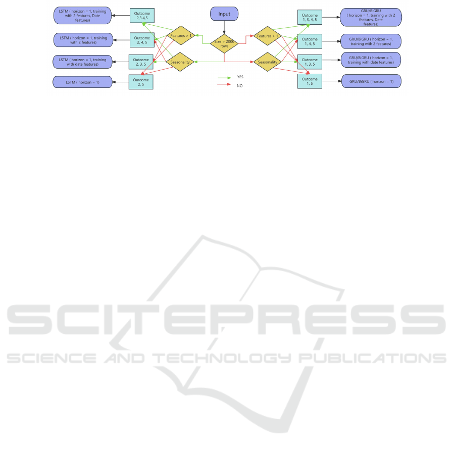
Figure 10: Decision Tree of Model Selection.
data make it challenging to analyze. Choose a suit-
able model among an abundance of proposed mod-
els is difficult. We conducted a series of experiments
to explore the relationship between the features of
datasets and the models and to thoroughly inquire if
we can select a suitable model based on the character-
istics of input datasets. We chose five kinds of mod-
els and two datasets with different characteristics to
conduct experiments and applied eight types of set-
tings for each model, aiming to find the best parame-
ters setup. Finally, we acquired a series of outcomes
that are the foundation for selecting a proper model
for a time-series dataset. We also proposed several
phenomenons on how these outcomes can be used
correctly. We designed a decision tree that outputs
a recommendation of the most suitable model based
on the characteristics of the input dataset. Moreover,
these outcomes can be used as meta-information in
the training process to design an Automated Model
Selection Technique.
We continue working on the outcomes we got. We
intend to employ more datasets and models to acquire
more accurate and general outcomes. At the same
time, some test experiments can be employed to ex-
amine the accuracy of outcomes.
REFERENCES
atoti (2024). When to perform a feature scaling. Accessed:
2024-01-24.
Bentaleb, A., Begen, A. C., Harous, S., and Zimmermann,
R. (2020). Data-driven bandwidth prediction models
and automated model selection for low latency. IEEE
Transactions on Multimedia, 23:2588–2601.
bmonikraj (2023). Medium-ds-unsupervised-anomaly-
detection-deepant-lstmae. Accessed: 2023-12-21.
Box, G. E. and Tiao, G. C. (1975). Intervention analy-
sis with applications to economic and environmental
problems. Journal of the American Statistical associ-
ation, 70(349):70–79.
Calcagno, V. and de Mazancourt, C. (2010). glmulti: an
r package for easy automated model selection with
(generalized) linear models. Journal of statistical soft-
ware, 34:1–29.
csafrit2 (2023). Steel industry energy consumption. Ac-
cessed: 2023-12-21.
dotdata (2024). Practical guide for feature engineering of
time series data. Accessed: 2024-02-02.
Esling, P. and Agon, C. (2012). Time-series data mining.
ACM Computing Surveys (CSUR), 45(1):1–34.
Iwasaki, Y. and Levy, A. Y. (1994). Automated model selec-
tion for simulation. In AAAI, pages 1183–1190. Cite-
seer.
Kotthoff, L., Thornton, C., Hoos, H. H., Hutter, F., and
Leyton-Brown, K. (2017). Auto-weka 2.0: Auto-
matic model selection and hyperparameter optimiza-
tion in weka. Journal of Machine Learning Research,
18(25):1–5.
Mahalakshmi, G., Sridevi, S., and Rajaram, S. (2016). A
survey on forecasting of time series data. In 2016
international conference on computing technologies
and intelligent data engineering (ICCTIDE’16), pages
1–8. IEEE.
Malkomes, G., Schaff, C., and Garnett, R. (2016). Bayesian
optimization for automated model selection. Ad-
vances in neural information processing systems, 29.
Mondal, P., Shit, L., and Goswami, S. (2014). Study of
effectiveness of time series modeling (arima) in fore-
casting stock prices. International Journal of Com-
puter Science, Engineering and Applications, 4(2):13.
Peixeiro, M. (2022). Time series forecasting in python. Si-
mon and Schuster.
Robikscube (2023). Hourly energy consumption. Accessed:
2023-12-20.
Saleem, S. and Kumarapathirage, S. (2023). Autonlp: A
framework for automated model selection in natural
language processing. In 2023 18th Iberian Conference
on Information Systems and Technologies (CISTI),
pages 1–4. IEEE.
Schuster, M. and Paliwal, K. K. (1997). Bidirectional re-
current neural networks. IEEE transactions on Signal
Processing, 45(11):2673–2681.
Shchur, O., Turkmen, A. C., Erickson, N., Shen, H.,
Shirkov, A., Hu, T., and Wang, B. (2023). Autogluon–
timeseries: Automl for probabilistic time series fore-
casting. In International Conference on Automated
Machine Learning, pages 9–1. PMLR.
sumanthvrao (2023). Daily climate time series data. Ac-
cessed: 2023-12-21.
Wang, C., Chen, X., Wu, C., and Wang, H. (2022). Au-
tots: Automatic time series forecasting model de-
sign based on two-stage pruning. arXiv preprint
arXiv:2203.14169.
Ying, Y., Duan, J., Wang, C., Wang, Y., Huang, C., and Xu,
B. (2020). Automated model selection for time-series
anomaly detection. arXiv preprint arXiv:2009.04395.
Towards the Automated Selection of ML Models for Time-Series Data Forecasting
819