Neural Architecture Search: Tradeoff Between Performance and
Efficiency
Tien Dung Nguyen
1
, Nassim Mokhtari
2 a
and Alexis N
´
ed
´
elec
2 b
1
University of Western Brittany, Brest, 29200, France
2
European Center for Virtual Reality, Brest National School of Engineering, Brest, 29200, France
Keywords:
Neural Architecture Search, Training-Free, Efficient Neural Network, AutoML, Multi-objectives
Optimization.
Abstract:
Many Neural Architecture Search (NAS) methods have designed models that outperform manually configured
networks on various tasks. Due to computational cost of model’s training, recent trend includes performing
NAS without training candidate networks in the process. Many such methods have proven that training-free
metrics are an effective way to assess model’s performance, especially if they are combined together. Multi-
training-free-objectives NAS methods usually construct a Pareto front that gives a wide range of solutions.
However, only one solution is chosen in the end. We introduce the Rank-based Improved Firefly Algorithm
(RB-IFA), which focuses the search in a single direction by converting multiple objective ranks into one
weighted sum. Weights are derived from a performance-efficiency tradeoff. Our search algorithm is based on
an Improved Firefly Algorithm (IFA). IFA effectively explores the NAS landscape by combining the Firefly
Algorithm, which has fast convergence, with a genetic algorithm, which improves the ability to overcome
local optima. RB-IFA NAS identifies highly efficient architectures with competitive performance within 8
minutes. These results highlight the potential of multi-training-free metrics and a rank-based approach in
finding efficient neural networks.
1 INTRODUCTION
Deep learning has found application in increasingly
complex problems, necessitating the development of
larger and more intricate models to effectively cap-
ture complex patterns and representations (Wei et al.,
2022; Simonyan and Zisserman, 2015). This shift has
made the manual design of new architectures increas-
ingly time-consuming (Elsken et al., 2019), which
motivates the community to automate the design pro-
cess by introducing new methods, such as Neural Ar-
chitecture Search (NAS).
Neural architecture search, a sub-field of auto-
mated machine learning (AutoML), involves auto-
matically seeking high quality deep neural networks
(DNNs) for a specific task on certain datasets (Elsken
et al., 2019). NAS generally consists of three steps:
first defining a search space in which a solution (ar-
chitecture) can be found; then defining a strategy to
sample candidates from the search space; and finally
a
https://orcid.org/0000-0002-9402-3638
b
https://orcid.org/0000-0003-3970-004X
assessing their performance. The sampling could be
repeated until the best solution is found, or a condition
is met.
In recent years, the field of Neural Architecture
Search has gained significant attention in the machine
learning community. Besides, the exponential growth
in computational resources required for training and
evaluating neural networks has led researchers to seek
alternative approaches that can identify optimal archi-
tectures without the need for extensive training cycles
(Mellor et al., 2021). More recently, a NAS approach
has been successfully applied to find image classifica-
tion models without training by using an Intra-Cluster
Distance (ICD) based metric to asses models’ qual-
ity, combined with an improved version of the Firefly
Algorithm (IFA) used as a search strategy (Mokhtari
et al., 2022).
Moreover, the energy consumption and CO
2e
emission of the training and the use of deep neural
network is also a concern to the environment (Strubell
et al., 2019). Thus, we need to prioritize efficiency
alongside performance when searching for new archi-
tectures. In this work, we explore the emerging land-
1154
Nguyen, T. D., Mokhtari, N. and Nédélec, A.
Neural Architecture Search: Tradeoff Between Performance and Efficiency.
DOI: 10.5220/0013296900003890
Paper published under CC license (CC BY-NC-ND 4.0)
In Proceedings of the 17th International Conference on Agents and Artificial Intelligence (ICAART 2025) - Volume 3, pages 1154-1163
ISBN: 978-989-758-737-5; ISSN: 2184-433X
Proceedings Copyright © 2025 by SCITEPRESS – Science and Technology Publications, Lda.

scape of training-free NAS methods, with a particular
focus on incorporating efficiency as a key criterion in
the search process.
Because NAS usually deals with balancing con-
flicting objectives like performance and efficiency, it
often uses Multi-objective Optimization (MOO) (Lu-
ong et al., 2024; Do and Luong, 2021). As no sin-
gle solution typically optimizes all objectives, the fo-
cus is on Pareto optimal solutions - those that can’t
be improved in one objective without compromising
another. Evolutionary Multi-objective Optimization
(EMO) algorithms (Zitzler, 2012), including those
in NAS, use Pareto-based ranking to evaluate solu-
tions (Abdelfattah et al., 2021; Luong et al., 2024).
While Pareto-based NAS methods provide a range of
near-optimal models representing different trade-offs,
practical applications often require selecting only a
single best model.
The main contribution of this paper is the imple-
mentation of rank-based IFA with multiple training-
free metrics. We used two training-free metrics (Intra-
Cluster Distance (ICD) (Mokhtari et al., 2022) and
Synaptic Flow (Synflow) (Tanaka et al., 2020)) as
performance indicators, Floating Point Operations
(FLOPs) as cost penalty. However, instead of find-
ing a Pareto front of all near-optimal solutions and
discard most of them later, our method first decide
what the best performance-efficiency tradeoff is, then
search only in that direction.
The rest of the document is organised as follows:
Section 2 introduces a synthesis of the various works
relating multi-objectives training-free NAS. Section 3
will present the Rank-based Improved Firefly Algo-
rithm and its ranking mechanism. In Section 4, we
will present and discuss the results obtained on two
NAS benchmarks, showing the effectiveness of our
method. Finally, we will summarize in Section 5 the
conclusions of this work as well as the possible im-
provements.
2 RELATED WORKS
In this section we will review existing work related to
training-free multi-objectives optimization to search
for efficient neural architectures. First, we will ex-
plain Neural Architecture Search in general. Then,
we present existing methods for each component of
training-free NAS: search space, search strategy and
score functions.
2.1 Neural Architecture Search
If we oversimplify NAS as ”finding values of variable
X that minimize/maximize f (X)”, then:
1. The search space is analogous to the domain of
variable X, where each value of X represents a
possible architecture. In another word, the search
space of Neural Architecture Search refers to the
set of all possible neural network architectures
that can be explored and evaluated to find an opti-
mal architecture for a given task.
2. The search strategy is an algorithm or heuristic
that helps us find the architecture X that maxi-
mizes or minimizes f ().
3. f () is the metric that tells us if the architecture
X is good enough. This could be the test ac-
curacy of the network, or performance indica-
tor, or a combination of multiple metrics f (X) =
g( f
′
1
(X), f
′
2
(X), ..., f
′
n
(X)), where f
′
i
() are usually
performance indicators, but they could also be ef-
ficiency indicators.
2.2 Search Space
The first dimension of NAS is the search space. A
search space of NAS is a domain containing all possi-
ble neural architectures that NAS method might dis-
cover. A search space is typically defined by various
architectural hyper-parameters such as the number of
layers, types of operation for each layer, their configu-
rations and their connections. This causes the number
of possible architectures in the search space explodes
as the configuration freedom and the size of individ-
ual architectures increases. Thus, designing a search
space comes down to a exploration-exploitation trade-
off: exploring a smaller search space is less compu-
tationally expensive, but might limit the discovery of
truly novel and optimal architectures.
There are several NAS search spaces, such as
NAS-BENCH-101 (Ying et al., 2019) and NAS-
BENCH-201 (Dong and Yang, 2020). Both of them
are based on the repetition of blocks (stacks and cells)
and operations (see Figure 1).
These search spaces enable direct comparison
with existing NAS research, guaranteeing credible
and easily comparable results. These benchmarks
also provide pre-calculated performance metrics, re-
ducing computational costs and accelerating the de-
velopment cycle by eliminating the need for repeated
training.
Neural Architecture Search: Tradeoff Between Performance and Efficiency
1155

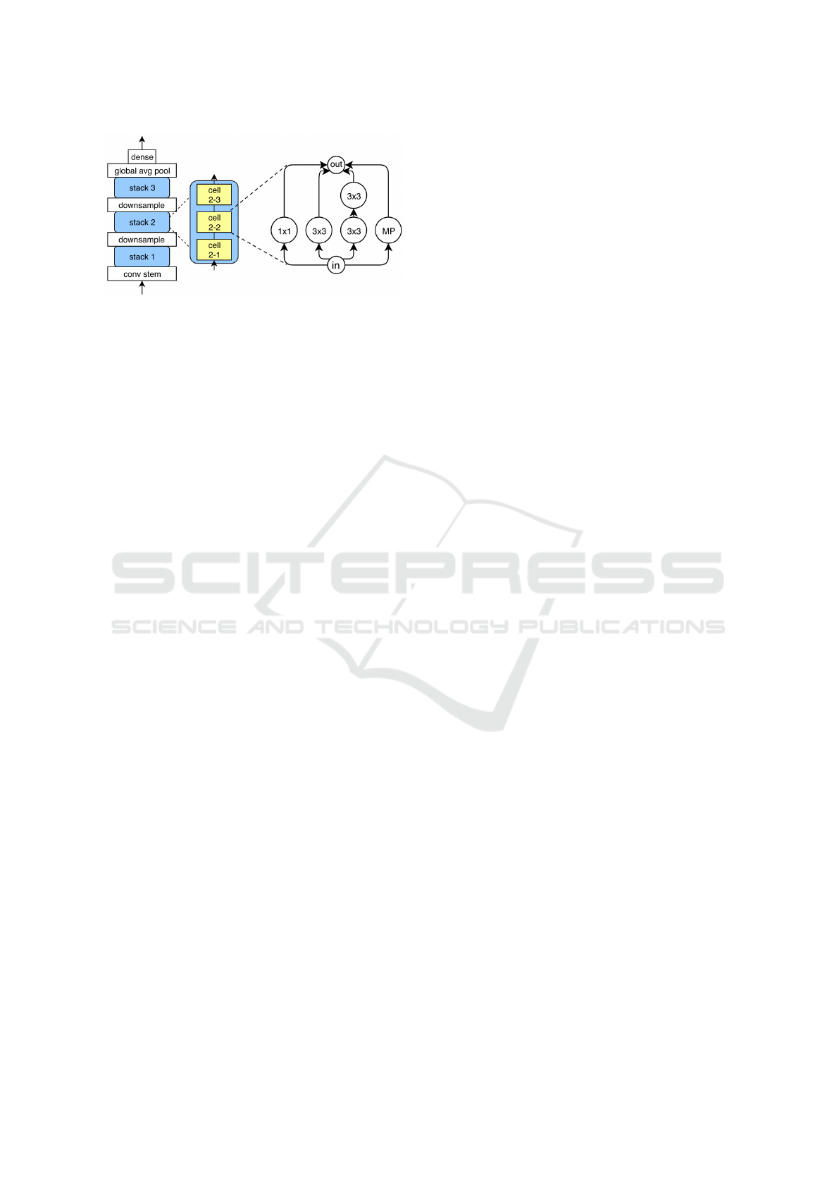
Figure 1: NASBench 101 architecture, (left) The outer
skeleton of each model. (right) An Inception-like cell with
the original 5x5 convolution approximated by two 3x3 con-
volutions (concatenation and projection operations omitted)
(Ying et al., 2019).
2.3 Search Strategy
The second and arguably the most important dimen-
sion of NAS is its search strategy. (Elsken et al., 2017)
propose a simple greedy search algorithm called hill
climbing that could serve as a good baseline search
strategy. (Elsken et al., 2017) theorize that because
NAS landscapes have a relatively low number of local
optima, this algorithm discovers high quality architec-
tures by simply moving toward direction of better per-
formance. (Phan and Luong, 2021) find better archi-
tectures by performing local search after finding po-
tential candidates, further prove that the search space
is rather smooth.
Early NAS method often use Reinforcement
Learning (RL), where a controller (agent) learns to
explore the search space efficiently (Zoph and Le,
2017; Zoph et al., 2018; Baker et al., 2017). The
generation of a neural architecture can be considered
to be the agent’s action, with the action space identi-
cal to the search space. For example, (Zoph and Le,
2017) use a recurrent neural network (RNN) policy to
sequentially sample a string that encodes the neural
architecture.
Beside RL, Evolutionary Algorithms (EAs) are
widely used due to the discreet nature of NAS search
spaces and their ease of implementation. Inspired by
the process of natural selection, EAs follow the prin-
ciple of Darwinism. In each population, individuals
with better fit have a higher chance of survival, op-
tionally mate and give offspring, who inherit charac-
teristics of their parents. This selection and inheri-
tance mechanism ensures the overall fit of the popu-
lation evolves over generations (iterations). There is
also a notion of mutation that potentially introduces
new characteristics to the population, avoiding local
optima.
(Mokhtari et al., 2022) combined Genetic Al-
gorithm (GA) with Firefly Algorithm (FA) (Yang,
2010b) creating Improved Firefly Algorithm (IFA). In
FA, a firefly is equivalent to a neural network. Each
firefly’s position corresponds to the architecture’s po-
sition in the search space. Fireflies that are close to-
gether represent architectures with similar structure.
Each firefly is attracted to brighter (better fitted) ones,
and move toward them. Light intensity is decrease
over long distance, this decrease depends on a light
absorption coefficient γ. IFA has the same mecha-
nism, but once the algorithm gets stuck in a local op-
timum, (Mokhtari et al., 2022) introduce a genetic it-
eration (selection, mating and mutation).
(Real et al., 2019) compare RL and EA and found
that they perform equally well in terms of test accu-
racy of architectures found. But EA have a better any-
time performance and find smaller architectures.
We decided to use the IFA as a search strategy,
as according to (Elsken et al., 2017), greedy search
might be a good strategy to achieve faster conver-
gence while not sacrificing a lot of performance. IFA
is the perfect candidate to test that hypothesis: it is
easy to adjust the greediness of FA so that it behaves
similarly to different metaheuristics, from random
search to Particle Swarm Optimization (PSO) (Yang,
2010a). For example, if we set the light absorption
coefficient γ to ∞, the fireflies do not see light, thus
there is no attractiveness and they wander randomly,
making FA behaves like random search. If γ is set
to 0, every firefly will see the global best and move
toward it, FA in this case is similar to PSO. Moder-
ate γ would make fireflies to aggregate closely around
different local optima. The genetic iteration in IFA
acts as a safety measure to avoid getting stuck in a lo-
cal optima for too long, which is common in greedy
search algorithms.
2.4 Performance Metrics
Traditionally, f () is the test accuracy of the network
after fully trained (Zoph and Le, 2017; Zoph et al.,
2018; Real et al., 2018). Then, to reduce computation
cost, NAS methods use single proxy function f
′
() to
estimate the real performance of networks without or
with very little training (Mellor et al., 2021; Mokhtari
et al., 2022; Abdelfattah et al., 2021). In recent pa-
per, (Luong et al., 2024) proves multi-training-free
metrics (Synflow (Mellor et al., 2021), Jacov (Tanaka
et al., 2020)) to be superior to single metric at esti-
mating model’s performance, while being extremely
fast.
Below is a brief description of the measures iden-
tified in our research :
1. Jacobian Covariance (JACOV) (Mellor et al.,
2021): This indicator assesses network perfor-
ICAART 2025 - 17th International Conference on Agents and Artificial Intelligence
1156

mance by measuring dissimilarity between binary
activation patterns of two inputs at each ReLU
layer. It evaluates the network’s ability to disen-
tangle input data, since for the same batch of data,
networks with higher capacity to distinguish two
inputs is more likely to have dissimilar activation
patterns. Given a mini-batch of data X = {x
i
}
N
i=1
mapped through the neural network, the binary
code c
i
associated with input x
i
defines the linear
region in which x
i
lies. The Hamming distance
d
H
(c
i
, c
j
) between the binary codes c
i
and c
j
for
two inputs x
i
and x
j
measures the dissimilarity as-
sociated with these inputs. One of the limitations
of JACOV is that it can only be used in ReLU net-
works, and can be computationally very expen-
sive, especially for large networks and large batch
sizes.
2. ICD: (Mokhtari et al., 2022) argue that a bi-
nary code generated from other layers than ReLU
could also be used to assess the way models inter-
prets the inputs. To measure the dissimilarity be-
tween binary activation, they compute ICD which
is the Euclidean distance d between each binary
code c
i
and the center
¯
c
ICD =
1
N
N
∑
i=1
d(
¯
c, c
i
) (1)
3. SNIP (Single-shot Network Pruning) (Lee et al.,
2019): SNIP is a method for pruning network
weights based on their saliency, a sensitivity cri-
terion to evaluate how much each weight con-
tributes to the loss function at initialization. It is
computed using the gradient of the loss with re-
spect to each weight’s mask c. The saliency for
a weight S
p
(w) is defined as the Hadamard prod-
uct (element-wise multiplication) ⊙ of the weight
value w and its mask’s gradient
∂L
∂c
. The overall
snip score for the entire network S
n
is obtained
by summing their saliency S
p
values over all pa-
rameters (N):
S
n
=
N
∑
i=1
S
p
(w
i
) (2)
This network score is also computed in the same
manner for other metrics that rely on saliency.
SNIP is simple to implement, but it approximate
the change in loss by considering only the gradi-
ent of the masks when they are all 1.
4. Synaptic Flow (Synflow) (Tanaka et al., 2020):
The key intuition is based on the principle of con-
serving the ”flow” of synaptic strength through
the network. This flow is analogous to the flow of
current in electrical circuits. Unlike other metrics
that depend on the training data, synflow passes
an input with all values equal to 1 through the net-
work. The output will be equal to the product of
every layer’s parameters, and will be used as the
loss. This loss function L is given by:
L = 1
T
L
∏
l=1
|θ
[l]
|
!
1 (3)
where 1 is the all-one vector, θ denotes the param-
eters of the network, and θ
[l]
represents the param-
eter values in the l-th layer.
The synflow saliency score for an architecture
with n parameters is computed as the element-
wise product ⊙ of the gradient of the loss function
L with respect to the parameter θ and the param-
eter’s value θ:
S
p
(θ) =
∂L
∂θ
⊙ θ (4)
Synflow is data-independent, however, it may suf-
fer from gradient explosion. But that could be al-
leviated by computing the log of gradient instead
(Cavagnero et al., 2023).
(Luong et al., 2024) showed that the quality of ap-
proximation fronts obtained using Synflow as objec-
tives is significantly better than those obtained when
optimizing other training-free performance metrics
(i.e, SNIP, GRASP (Wang et al., 2020), FISHER
(Theis et al., 2018) and JACOV).
Approximation fronts are Pareto fronts obtained
using training-free metrics and one complexity met-
ric. We chose Synflow due to its proven effective-
ness. But Synflow is a data-agnostic metric. Whereas,
according to No Free Lunch Theorem (Goodfel-
low et al., 2016), across different task, no machine
learning algorithm is universally superior to another.
Thus, beside Synflow, we need a metric that cap-
tures data complexity and probability distribution.
ICD is a good candidate since it is data dependant,
but unlike JACOV it is independent on ReLU acti-
vation thanks to its binary code generation mecha-
nism. Furthermore, ICD has good Spearman corre-
lation with test accuracy: 0.52 and 0.63 for archi-
tectures in NAS-Bench-101 and NAS-Bench-201 re-
spectively. While Synflow has Spearman correlation
coefficient of NAS-Bench-101 and NAS-Bench-201
architectures of 0.37 and 0.74 respectively. So we
decided to experiment with Synflow and additionally
ICD as two performance metrics.
2.5 Complexity Measures
Besides performance indicators complexity measures
are often used as penalty in order to find efficient
Neural Architecture Search: Tradeoff Between Performance and Efficiency
1157

architectures in multi-objectives NAS(Luong et al.,
2024):
• Number of parameters: This is a simple yet ef-
fective measure, where complexity is directly pro-
portional to the number of trainable parameters
in the network (Laredo et al., 2019). However,
it doesn’t consider the structure or connectivity
of the architecture, or the recurrence nature of a
network, and measuring model complexity by the
number of trainable parameters has a very lim-
ited effect on deep learning models since deep
learning models are often over-parameterized (Hu
et al., 2021). Parameter count also does not take
into account sequence length in case of a RNN.
• Number of FLOPs (Floating-point Operations)
(Tan and Le, 2020): This measure estimates the
computational cost of the network by counting
the number of basic floating point operations of
the form a ∗ b + c. It provides a better estima-
tion of complexity than parameter count, while
being easy to compute. Thus, this metric is widely
used to assess architecture’s complexity in NAS.
But the first downside of FLOPs is that operations
like divisions, reciprocals, square roots, log, ex-
ponential, etc, are too expensive to include as a
single operation, while activation functions do af-
fect computation complexity, but are not counted
as one operation. Besides, model’s sparsity could
reduce computational cost, but is not reflected in
FLOP count.
• Number of linear regions (Chen et al., 2021):
Linear region is a contiguous area within this in-
put space where the neural network’s behavior can
be represented by a linear function. By dividing
the input space into these linear regions, the neu-
ral network can approximate complex functions.
The more linear regions a neural network can de-
fine, the more flexible and capable it is in captur-
ing intricate patterns in the data. A limitation of
this metric is that it is hard to compute, especially
for large networks.
• Cost to generate a result (Schwartz et al., 2019):
This is the estimation of the cost to produce an
AI result reported in a scientific paper, which of-
ten involves multiple experiments to tune a model
hyperparameters:
Cost(R) ∝ E · D · H (5)
where:
– E is the cost of executing the model on a single
(E)xample,
– D is the size of the training (D)ataset,
– H is the number of (H)yperparameter experi-
ments.
However, since we typically run NAS to find good
architectures for one dataset, and architectures
found also follow the same training pipeline, it is
more practical to take into account only the train-
ing, or inference time of architectures on a single
example.
We opt to use FLOP count as complexity measure due
to its ease to compute, its reliability compared to pa-
rameter count, and its device-agnostic nature.
3 METHOD
Improved Firefly Algorithm (IFA), proposed by
(Mokhtari et al., 2022), results in a focused and accel-
erated search process. Since IFA derives from Fire-
fly Algorithm (Yang, 2010b), which is similar to a
greedy search or local search. Each solution, or fire-
fly, moves towards better solutions based on a combi-
nation of their rank (brightness) and spatial distance
(architecture difference), ensuring that the search is
directed towards promising regions of the solution
space. When the best solution does not change for
some generation, IFA introduces genetic operations:
selection, mating, and mutation, to generate new pop-
ulations, thereby escaping local optima and maintain-
ing diversity in the search process.
To be able to use multiple training-free metrics, to
guide the search to a desired direction and to allevi-
ate the difference in ranges between different metrics
(ICD is in the range of hundreds, FLOPs counted at
millions), we add a new rank based mechanism. Each
Rank-based IFA execution starts with a performance
weight between 0 and 1, configured manually (default
is 0.5). The sum of efficiency weight and performance
weight is 1. Then, each performance metric is at-
tributed a weight by dividing the performance weight
by number of performance metrics. Similarly, for
each efficiency metric, its weight is the factor between
efficiency weight and number of efficiency metrics.
Lastly, for each metric (to minimize), we rank each
solution in ascending order. Each solution’s overall
rank is a weighted sum of its individual metric ranks.
The lower the rank, the better. The following formula
illustrates how the rank of a solution is computed:
R
solution
=
(R
ICD
+ R
Syn f low
) ∗W
p
2
+R
FLOPs
∗W
e
(6)
Where R
solution
is the rank of the solution in the pop-
ulation, R
ICD
, R
Syn f low
and R
FLOPs
are its individual
negative ICD, negative Synflow and FLOPs ranks re-
ICAART 2025 - 17th International Conference on Agents and Artificial Intelligence
1158

spectively, W
p
and W
e
are performance and efficiency
weights (W
p
+W
e
= 1).
Since in the initial population, the overall quality
of solutions is not great, a mediocre solution A could
achieve low ranking (the lower the better). Whereas,
in later generation, a solution B better than A might
not achieve lower ranking than A because B has to
compete with solutions of better quality. Thus, we
have to reset the ranking once the algorithm got stuck
and unable to find a lower rank solution.
To demonstrate the effectiveness of rank-based
IFA, we benchmark it against a Pareto-front IFA (PF-
IFA) (algorithm 1). Instead of incorporating all objec-
tive into one ranking, we construct a Pareto front of
the population using Non-dominated Sort with dom-
inance degree. This is a method used to rank so-
lutions in a population based on their level of non-
domination. Solutions that are not dominated by any
other solutions are assigned rank 0 (the best rank).
Then, these solutions are temporarily removed, and
the process is repeated to find the next set of non-
dominated solutions (rank 1), and so on.
Algorithm 1: Pareto front Improved FireFly Algorithm.
Randomly generate the population
Define MaxChances
Define PopulationSize
chances = MaxChances
population.size = PopulationSize
candidates = [ ]
pareto f ront size = 0
while not Stopping criteria do
Running an iteration of FireFly Algorithm
pareto f ront = current population’s non domi-
nated solutions
if pareto f ront size < size(pareto f ront) then
pareto f ront size = size(pareto f ront)
population.size = PopulationSize +
pareto f ront size
else
chances–
end if
if chances=0 then
Perform an iteration of the Genetic Algorithm
chances = MaxChances
end if
end while
candidates = pareto f ront
Determining the best solution from the candidates
list
We use the size of the Pareto front as a simple in-
dicator to tell if the population advances in the de-
sired direction (minimize all metric), or get stuck in
the metric scores space. Although it is not always the
case that a larger number of solutions in the Pareto
front means better front quality, this approach is much
simpler than using Hyper Volume. The latter is a mea-
sure of the volume between the front’s points and a
worst reference point. It represents more reliably the
advancement of solutions toward better quality, but it
is also costly to compute, especially when the number
of metrics is high.
The source code will be made public upon accep-
tance of the paper.
4 EXPERIMENTATION AND
DISCUSSION
In this section, we will assess the performance of
Rank-Based IFA (RB-IFA), comparing its results to
its counterpart Pareto front IFA (PF-IFA), using ICD,
Synflow and FLOPs as metrics.
First, we will demonstrate the benefit of using
multiple training-free performance metric (ICD, Syn-
flow) instead of one. Then, we will compare the per-
formance of RB-IFA and PF-IFA on NAS-Bench-101
and NAS-Bench-201.
4.1 Multiple Training-Free
Performance Metric
We first run RB-IFA with three different metrics con-
figuration:
• ICD, Synflow, FLOPs
• ICD, FLOPs
• Synflow, FLOPs
For each configuration, we first run the algorithm 50
times: 10 times per performance weight (0.25, 0.33,
0.5, 0.66). The best solutions found amongst 10 runs
(in terms of test accuracy) are showed in figures 2, 3
and 4.
We observe that the first and second configuration
found solutions with better accuracy than the third
one (Synflow-FLOPs). The figures also showed that
method with two performance metrics navigates bet-
ter in the performance-efficiency space. Since the so-
lutions found in the first diagram (figure 2) is ordered
according to their performance-efficiency tradeoff.
Whereas, solutions of Synflow-FLOPs are clumped
up together, and solutions of ICD-FLOPs do not fol-
low the order of their performance weight.
Next we run three similar configurations, but with
PF-IFA, to construct three Pareto fronts. Each con-
figuration is also repeated 10 times. Figure 5 show
Neural Architecture Search: Tradeoff Between Performance and Efficiency
1159

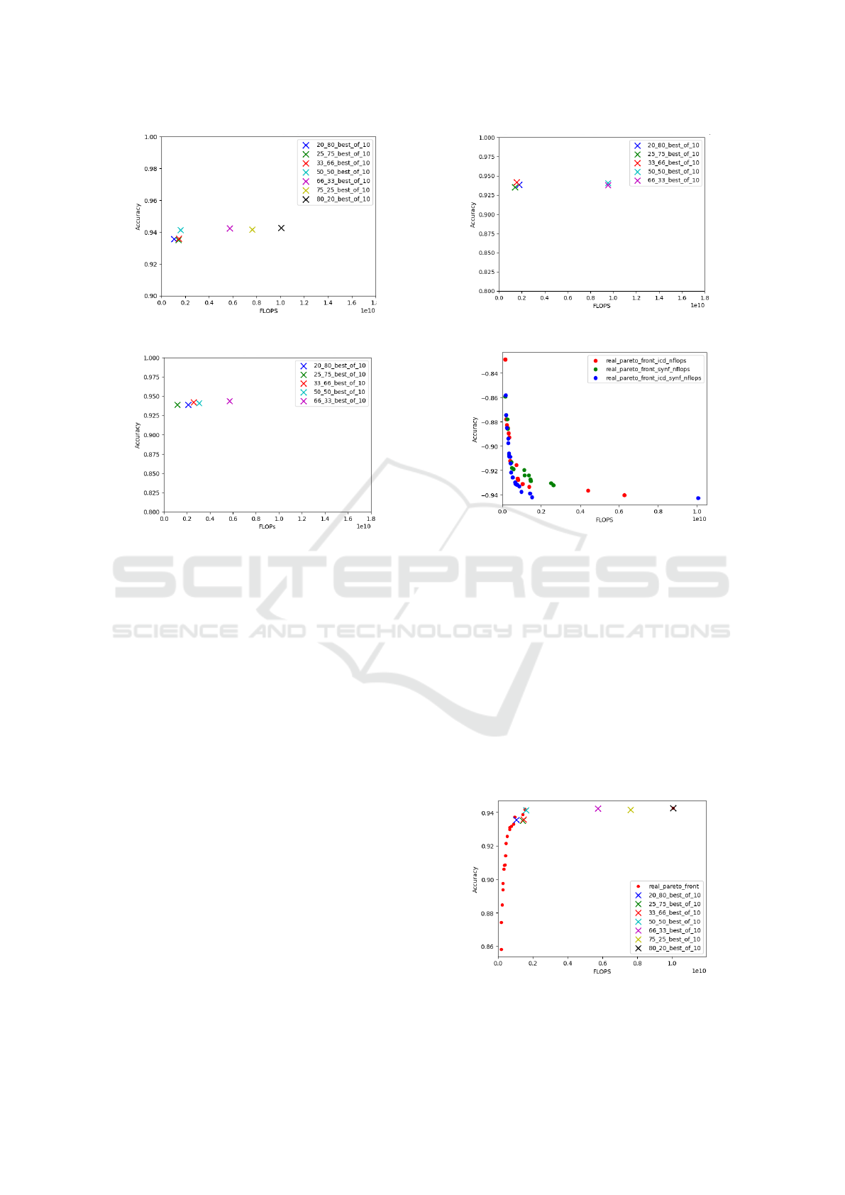
Figure 2: Best solutions obtained by ICD+Synflow+FLOPs.
Figure 3: Best solutions obtained by ICD+FLOPs.
that the Pareto front created by ICD-Synflow-FLOPs
advances faster and further than the others, with ICD-
FLOPs in the second and Synflow-FLOPs comes last.
This result is consistent with the results of (Luong
et al., 2024) and (Abdelfattah et al., 2021).
4.2 RB-IFA vs PF-IFA
Knowing that two performance metrics work better
than single one, we compare three metrics RB-IFA
and three metrics PF-IFA with data we gathered so
far in figure 6. The data showcase that PF-IFA’s so-
lutions lack diversity in plateau regions, whereas RB-
IFA could find solutions in any direction, depending
on the performance weight. This figure also provides
an insight for constructing a pseudo-Pareto front from
the RB-IFA solutions, by running RB-IFA on a wider
range of performance-efficiency tradeoff. And then,
combine their solutions and construct a pseudo-Pareto
front using Dominance Degree Non-Dominated Sort.
If RB-IFA is more focused and progresses faster to-
ward the optima, the Hyper Volume (HV) of the
pseudo-Pareto front after the same runtime will be
greater than that of PF-IFA. This implies that, at a
given time t, the best solution found by RB-IFA is
likely to surpass the Pareto front of PF-IFA. Surpass-
ing a Pareto front means dominating at least one solu-
tion on that front
Figure 4: Best solutions obtained by Synflow+FLOPs.
Figure 5: Three Pareto fonts constructed by three differ-
ent configurations: ICD-Synflow-FLOPs, ICD-FLOPs and
Synflow-FLOPs.
We proceed by running RB-IFA with the NAS-
Bench 101 search space, at 19 different performance
weights, ranging from 0.05 to 1. Then the Hyper Vol-
umes (HV) over time of two algorithms are computed,
and shown in figure 7.
The figure shows that the quality of solution in
the pseudo-front is superior, and advance much faster
than those of the real front. We also obtain the same
results in NASBench 201 (figure 8).
We hypothesized that combining the solutions
from RB-IFA runs with different performance trade-
offs led to the creation of a better Pareto front, primar-
Figure 6: Comparing best solution found by RB-IFA at
different performance-efficiency tradeoff, and Pareto front
found by PF-IFA.
ICAART 2025 - 17th International Conference on Agents and Artificial Intelligence
1160

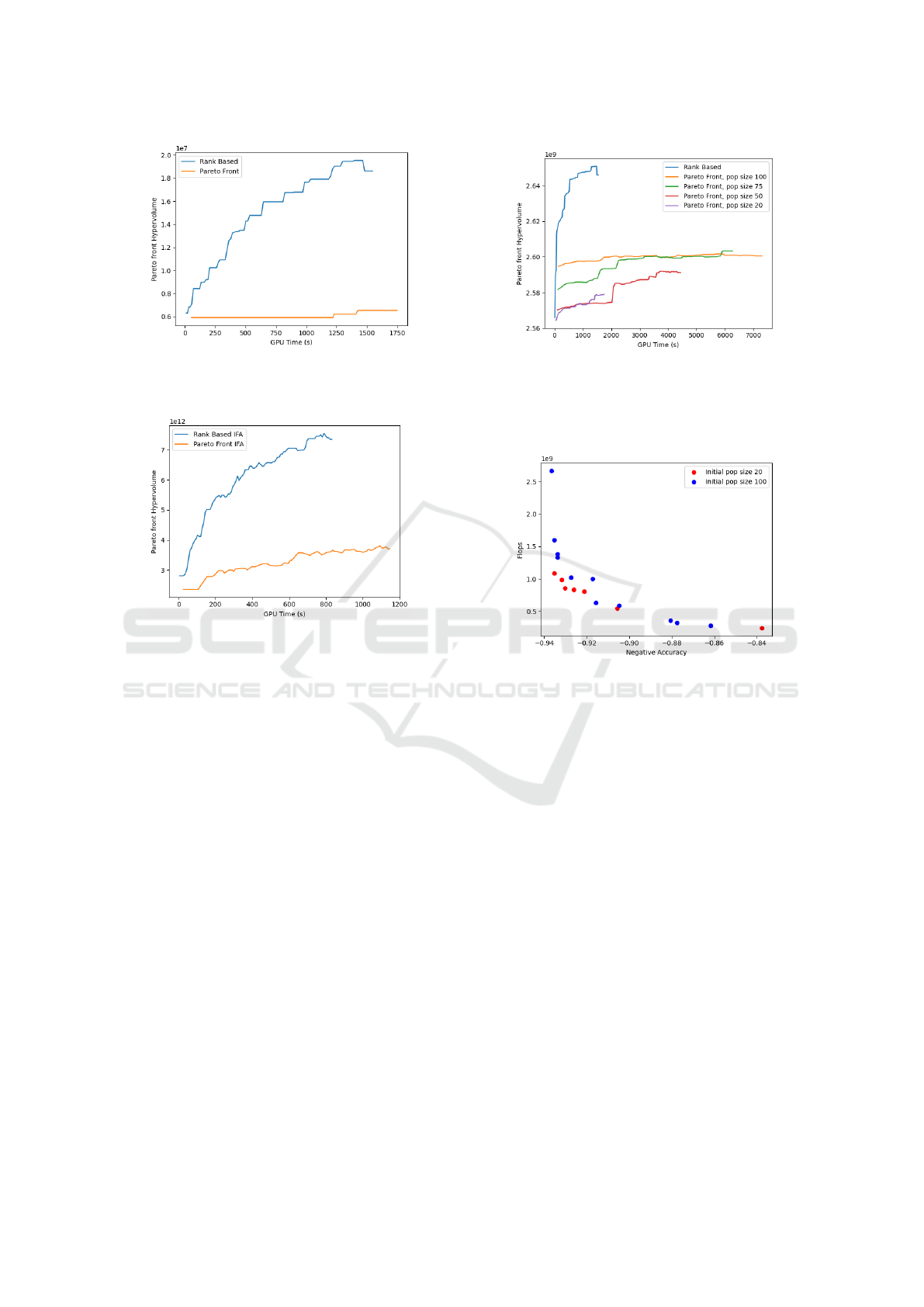
Figure 7: Average Hyper Volume (HV) over time of
pseudo-Pareto font constructed from RB-IFA solutions, and
Pareto front of PF-IFA, NASBench 101.
Figure 8: Average Hyper Volume (HV) over time of
pseudo-Pareto font constructed from RB-IFA solutions, and
Pareto front of PF-IFA, NASBench 201.
ily due to the larger number of solutions. However,
when running PF-IFA with different initial population
sizes (20, 75, 100), the results shows that RB-IFA still
have far faster convergence.
Figure 9 shows that Pareto front with higher pop-
ulation size starts off with bigger Hypervolume (be-
cause initialization time is not counted), but grows
very slowly. This is due to the fact that runs with
higher initial population sacrifice speed for diversity
on the Pareto front.
Figure 10 shows that even after less runtime, PF-
IFA with 100 initial population size found a more di-
verse Pareto front than PF-IFA with 20 initial solu-
tions, but is also gapped more by the pseudo-Pareto
front.
4.3 RB-IFA vs Other Methods
We use NASWOT (Mellor et al., 2021) as a baseline,
since it only select architecture at random and evalu-
ate them using single training-free metric (JACOV).
The results of table 1 are added later using an
NVIDIA GeForce RTX 3060, while figures 7, 8 and
9 are obtained using a NVIDIA GeForce GTX 1070.
Figure 9: Average Hyper Volume (HV) over time of
pseudo-Pareto font constructed from RB-IFA solutions (19
different performance tradeoff, population size 20), and
Pareto front of PF-IFA (initialized at different population
size).
Figure 10: PF-IFA tradeoff between diversity and speed:
after 230s runtime, PF-IFA with bigger initial population
size has a more diverse Pareto front, but converge slower.
Our inability to utilize the same hardware is the cause
of such discrepancy in execution time of our RB-IFA
algorithm.
Efficient Training-Free Multi-Objective Evolu-
tionary Neural Architecture Search (E-TF-MOENAS)
(Luong et al., 2024) is the most recent and also the
closest to our method, however, E-TF-MOENAS uses
NSGA-II and Pareto front, while we use IFA and a
rank-based approach. We also use three training-free
metrics, but with ICD in place of JACOV. To have
a direct comparison between our method and E-TF-
MOENAS , we run E-TF-MOENAS as normal, then
rank the final population using our ranking mecha-
nism (eq. 6). As a result, we also obtain the best archi-
tectures depending on the performance-cost tradeoff.
We focus on the most interesting tradeoffs: (50-50)
and (100-0). Table 1 shows that our method achieve
comparable results while taking much less time than
E-TF-MOENAS. This proves that focusing in one di-
rection from the beginning instead of advancing the
whole Pareto-front will accelerate the convergence of
the search process.
Neural Architecture Search: Tradeoff Between Performance and Efficiency
1161

Table 1: Comparison of different NAS methods on the
NAS-Bench 101 and NAS-Bench 201 search space for the
dataset CIFA10. (50-50) and (100-0) are performance-
complexity tradeoffs.
Algorithm Test Accuracy GFLOPs Cost (sec.)
NAS-Bench 101
Random-walk, single metric, training-free
NASWOT
(Mellor et al.,
2021)
91.77±0.05 0.18±0.02 23
Evolutionary algorithm, single objective, train-based
REA (Real et al.,
2018)
93.87±0.22 0.22±0.01 12 000
Evolutionary algorithm, multi-metrics, training-free
Performance-cost tradeoff: 50-50
E-TF-MOENAS 92.96±0.21 0.04±0.00 4 850
RB-IFA 93.64±0.20 0.05±0.00 484
Performance-cost tradeoff: 100-0
E-TF-MOENAS 93.98±0.08 0.16±0.02 4 850
RB-IFA 93.65±0.30 0.22±0.02 484
NAS-Bench 201
Random-walk, single metric, training-free
NASWOT
(Mellor et al.,
2021)
92.96±0.81 0.30±0.01 307
Evolutionary algorithm, single objective, train-based
REA (Real et al.,
2018)
93.92±0.30 0.29±0.05 12 000
Evolutionary algorithm, multi-metrics, training-free
Performance-cost tradeoff: 50-50
E-TF-MOENAS 93.51±0.39 0.15±0.02 11 874
RB-IFA 92.63±1.25 0.02±0.08 267
Performance-cost tradeoff: 100-0
E-TF-MOENAS 94.36±0.01 0.37±0.00 11 874
RB-IFA 93.68±1.15 0.27±0.03 267
Our method is superior to Regularized Evolution-
ary Algorithm (REA) (Real et al., 2018) in terms
of execution time while having comparable perfor-
mance. This further demonstrates the effectiveness
of multi-training-free-metrics approach. Moreover,
since REA particularly focus on avoiding greediness
of the search algorithm, this result proves that greedi-
ness does not hurt performance in NAS.
We can see that in table 1, a tradeoff of (50-50)
gives a 4.4 to 13.5 times reduction in model size while
sacrificing very little accuracy (0.01% to 1.05%).
5 CONCLUSION
In this work, we investigated the potential of using
multiple training-free metrics and a rank-based ap-
proach in Neural Architecture Search to find models
with good performance-efficiency tradeoff. The com-
bination of ICD and Synflow as performance met-
rics, along with FLOPs as an cost penalty for effi-
ciency, allowed RB-IFA to navigate the performance-
efficiency trade-off more effectively than single-
metric approaches.
The superiority of RB-IFA over PF-IFA (in terms
of Hypervolume) and over E-TF-MOENAS (in terms
of speed) highlight the focused nature of our ap-
proach. By allowing the population to move greed-
ily to a specific trade-off direction, we achieve faster
convergence towards optimal solutions in the desired
regions of the search space.
To further accelerate our search process, we’re
considering integrating a model generator using
GFlowNet (Bengio et al., 2023). GFlowNet allows
the generation diverse of graph-based elements fol-
lowing a probability distribution, instead of maxi-
mizing a score function. With the starting point de-
rived from our performance-efficiency tradeoff, this
approach would allow us to generate networks around
a desired complexity (FLOPs), without bias. By ini-
tializing our search with architectures in the search
direction, we could potentially make the search even
more focused and accelerate the process significantly.
Additionally, it would be valuable to develop a new
efficiency metric that assesses both the performance
and computational cost of a model, thereby simplify-
ing the process of selecting an optimal network.
ACKNOWLEDGEMENTS
This work has been carried out within the French-
Canadian project DOMAID which is funded by the
National Agency for Research (ANR-20-CE26-0014-
01) and the FRQSC.
REFERENCES
Abdelfattah, M. S., Mehrotra, A., Łukasz Dudziak, and
Lane, N. D. (2021). Zero-cost proxies for lightweight
nas.
Baker, B., Gupta, O., Naik, N., and Raskar, R. (2017).
Designing Neural Network Architectures using Rein-
forcement Learning. arXiv:1611.02167 [cs].
Bengio, Y., Lahlou, S., Deleu, T., Hu, E. J., Tiwari,
M., and Bengio, E. (2023). GFlowNet Foundations.
arXiv:2111.09266 [cs, stat].
Cavagnero, N., Robbiano, L., Caputo, B., and Averta, G.
(2023). FreeREA: Training-Free Evolution-based Ar-
chitecture Search. In 2023 IEEE/CVF Winter Con-
ference on Applications of Computer Vision (WACV),
pages 1493–1502. arXiv:2207.05135 [cs].
Chen, W., Gong, X., and Wang, Z. (2021). Neural architec-
ture search on imagenet in four gpu hours: A theoret-
ically inspired perspective.
Do, T. and Luong, N. H. (2021). Training-Free Multi-
objective Evolutionary Neural Architecture Search via
Neural Tangent Kernel and Number of Linear Re-
gions. In Neural Information Processing: 28th Inter-
national Conference, ICONIP 2021, Sanur, Bali, In-
ICAART 2025 - 17th International Conference on Agents and Artificial Intelligence
1162

donesia, December 8–12, 2021, Proceedings, Part II,
pages 335–347, Berlin, Heidelberg. Springer-Verlag.
event-place: Sanur, Bali, Indonesia.
Dong, X. and Yang, Y. (2020). Nas-bench-201: Extending
the scope of reproducible neural architecture search.
Elsken, T., Metzen, J., and Hutter, F. (2019). Neural archi-
tecture search: A survey. Journal of Machine Learn-
ing Research, 20.
Elsken, T., Metzen, J.-H., and Hutter, F. (2017). Simple
And Efficient Architecture Search for Convolutional
Neural Networks. arXiv:1711.04528 [cs, stat].
Goodfellow, I., Bengio, Y., and Courville, A. (2016). Deep
Learning. MIT Press.
Hu, X., Chu, L., Pei, J., Liu, W., and Bian, J. (2021).
Model Complexity of Deep Learning: A Survey.
arXiv:2103.05127 [cs].
Laredo, D., Qin, Y., Sch
¨
utze, O., and Sun, J.-Q. (2019).
Automatic Model Selection for Neural Networks.
arXiv:1905.06010 [cs, stat].
Lee, N., Ajanthan, T., and Torr, P. H. S. (2019). Snip:
Single-shot network pruning based on connection sen-
sitivity.
Luong, N. H., Phan, Q. M., Vo, A., Pham, T. N., and
Bui, D. T. (2024). Lightweight multi-objective evolu-
tionary neural architecture search with low-cost proxy
metrics. Information Sciences, 655:119856.
Mellor, J., Turner, J., Storkey, A., and Crowley, E. J.
(2021). Neural Architecture Search without Training.
arXiv:2006.04647 [cs, stat].
Mokhtari, N., Nedelec, A., Gilles, M., and De Loor, P.
(2022). Improving Neural Architecture Search by
Mixing a FireFly algorithm with a Training Free Eval-
uation. volume 2022-July.
Phan, Q. M. and Luong, N. H. (2021). Enhancing multi-
objective evolutionary neural architecture search with
surrogate models and potential point-guided local
searches. In Fujita, H., Selamat, A., Lin, J. C.-W.,
and Ali, M., editors, Advances and Trends in Artificial
Intelligence. Artificial Intelligence Practices, pages
460–472, Cham. Springer International Publishing.
Real, E., Aggarwal, A., Huang, Y., and Le, Q. V. (2018).
Regularized Evolution for Image Classifier Architec-
ture Search. Publisher: arXiv Version Number: 7.
Real, E., Aggarwal, A., Huang, Y., and Le, Q. V. (2019).
Aging Evolution for Image Classifier Architecture
Search. In AAAI Conference on Artificial Intelligence.
Schwartz, R., Dodge, J., Smith, N. A., and Etzioni, O.
(2019). Green AI. Publisher: arXiv Version Number:
3.
Simonyan, K. and Zisserman, A. (2015). Very Deep Con-
volutional Networks for Large-Scale Image Recogni-
tion. arXiv:1409.1556 [cs].
Strubell, E., Ganesh, A., and McCallum, A. (2019). Energy
and Policy Considerations for Deep Learning in NLP.
arXiv:1906.02243 [cs].
Tan, M. and Le, Q. V. (2020). EfficientNet: Rethinking
Model Scaling for Convolutional Neural Networks.
arXiv:1905.11946 [cs, stat].
Tanaka, H., Kunin, D., Yamins, D. L. K., and Ganguli, S.
(2020). Pruning neural networks without any data by
iteratively conserving synaptic flow.
Theis, L., Korshunova, I., Tejani, A., and Husz
´
ar, F. (2018).
Faster gaze prediction with dense networks and fisher
pruning.
Wang, C., Zhang, G., and Grosse, R. (2020). Picking
winning tickets before training by preserving gradient
flow.
Wei, J., Tay, Y., Bommasani, R., Raffel, C., Zoph,
B., Borgeaud, S., Yogatama, D., Bosma, M.,
Zhou, D., Metzler, D., Chi, E. H., Hashimoto, T.,
Vinyals, O., Liang, P., Dean, J., and Fedus, W.
(2022). Emergent Abilities of Large Language Mod-
els. arXiv:2206.07682 [cs].
Yang, X. (2010a). Nature-inspired Metaheuristic Algo-
rithms. Luniver Press.
Yang, X.-S. (2010b). Firefly algorithm, stochastic test func-
tions and design optimisation.
Ying, C., Klein, A., Real, E., Christiansen, E., Murphy, K.,
and Hutter, F. (2019). NAS-BENCH-101: Towards
reproducible neural architecture search. volume 2019-
June, pages 12334–12348.
Zitzler, E. (2012). Evolutionary Multiobjective Optimiza-
tion. In Rozenberg, G., B
˜
ACck, T., and Kok, J. N.,
editors, Handbook of Natural Computing, pages 871–
904. Springer Berlin Heidelberg, Berlin, Heidelberg.
Zoph, B. and Le, Q. V. (2017). Neural Architecture Search
with Reinforcement Learning. arXiv:1611.01578 [cs].
Zoph, B., Vasudevan, V., Shlens, J., and Le, Q. V. (2018).
Learning Transferable Architectures for Scalable Im-
age Recognition. arXiv:1707.07012 [cs, stat].
Neural Architecture Search: Tradeoff Between Performance and Efficiency
1163