Breast Density Estimation in Mammograms Using Unsupervised

Image Segmentation

Khaldoon Alhusari and Salam Dhou

Department of Computer Science and Engineering, American University of Sharjah, Sharjah, U.A.E.

Keywords: Breast Cancer, Breast Density, Mammograms, Unsupervised Learning, Segmentation.

Abstract: Breast cancer is very common, and early detection through mammography is paramount. Breast density, a

strong risk factor for breast cancer, can be estimated from mammograms. Current density estimation methods

can be subjective, labor-intensive, and proprietary. This work proposes a framework for breast density

estimation based on the unsupervised segmentation of mammograms. A state-of-the-art unsupervised image

segmentation algorithm is adopted for the purpose of breast density segmentation. Mammographic percent

density is estimated through a process of arithmetic division. The percentages are then discretized into

qualitative assessments of density (“Fatty” and “Dense”) using a thresholding approach. Evaluation reveals

robust segmentation at the pixel-level with silhouette scores averaging 0.95 and significant unsupervised

labeling quality at the per-image level with silhouette scores averaging 0.61. The proposed framework is

highly adaptable, generalizable, and non-subjective, and has the potential to be a beneficial support tool for

radiologists.

1 INTRODUCTION

Breast cancer remains a formidable global health

challenge, constituting 11.7% of all cancer cases with

alarming mortality rates (Sung et al., 2021). The

significance of early detection is underscored by its

potential to mitigate the risks associated with this

prevalent malignancy. Mammographic screening,

particularly through mammograms, stands out as a

pivotal diagnostic tool due to its efficacy in

identifying tumors before clinical symptoms

manifest. However, the efficacy of mammography is

intricately linked to breast density, a parameter

determined by the proportion of radio-dense,

fibroglandular tissue (Kallenberg et al., 2016). Higher

breast density complicates tumor identification,

particularly in cases where the mammogram appears

highly dense, making early detection less reliable

(Wengert et al., 2019). Despite its efficacy,

mammography introduces a critical concern—

radiation exposure. The risk, though minimal, is not

negligible, and it is exacerbated in women with larger

breasts of a higher density (Dhou et al., 2022).

The interpretative aspect of mammography

introduces another layer of complexity, especially

concerning breast density assessments. Radiologists

exhibit variability in determining breast density, with

notable subjectivity in cases of highly dense breasts

(Sprague et al., 2016). This subjectivity can lead to

missed cancer diagnoses and biased treatment

decisions, as evidenced by the tendency to opt for

more invasive procedures for extremely dense breasts

(Nazari & Mukherjee, 2018).

There are various methods of breast density

estimation in the literature. In practice, the most

common is a visual assessment method known as the

Breast Imaging-Reporting and Data System (BI-

RADS) (Sickles, EA, D’Orsi CJ, Bassett LW, 2013),

which classifies breasts into four qualitative density

categories. Other visual systems of measurement

exist, such as the Wolfe Classification (Wolfe, 1976),

the Tabár Classification (Gram et al., 1997), and the

Visual Analogue Scale (VAS) (Nahler, 2009). There

are also software-based methods for breast density

estimation, some of which are semi-automatic such as

the Cumulus software (Byng et al., 1994), and some

of which are fully automatic such as the Quantra

software (Hartman et al., 2008).

In addition, there are studies that use machine

learning to solve the problem of breast density

estimation. It is worth noting that, using

mammography, AI has been successful in performing

several vital tasks such as tumor detection,

Alhusari, K. and Dhou, S.

Breast Density Estimation in Mammograms Using Unsupervised Image Segmentation.

DOI: 10.5220/0013297500003912

Paper published under CC license (CC BY-NC-ND 4.0)

In Proceedings of the 20th International Joint Conference on Computer Vision, Imaging and Computer Graphics Theory and Applications (VISIGRAPP 2025) - Volume 3: VISAPP, pages

691-698

ISBN: 978-989-758-728-3; ISSN: 2184-4321

691

classification, image improvement and breast density

estimation (Dhou et al., 2024). In a relevant work,

(Arefan et al., 2015), nine statistical features are

extracted from preprocessed mammograms and fed

into a two-layer feed-forward neural network,

achieving high classification accuracy. The work in

(Saffari et al., 2020) employs a conditional generative

adversarial network (cGAN) in combination with a

convolutional neural network (CNN) to classify

mammograms into one of four density categories, and

achieves high agreement with expert assessment.

Further, there are methods that rely on the

segmentation of the mammogram to produce a

percentage estimate of mammographic density. These

can be area-based, relying on the 2-dimensional

appearance of mammograms (e.g., thresholding and

clustering), or volume-based, attempting to quantify

the volume of density within a breast by estimating

depth. Notable works include (Kallenberg et al.,

2016), which uses a convolutional sparse autoencoder

(CSAE) with softmax regression, and (Gudhe et al.,

2022), which employs a multitask deep learning

model that utilizes multilevel dilated residual blocks

and parallel dilated convolutions to enhance feature

extraction. Both of these works achieve significant

correlation with expert assessment.

Each of the detailed breast density estimation

methods has some merits, but is also liable to flaws.

Visual methods like BI-RADS are widely adopted but

subjective and labor-intensive. Breast density

software are convenient but present challenges in

relation to their proprietary nature, and are often

inconsistent with one another. Machine learning

methods show promise but rely on subjective label

data and often focus on BI-RADS classification rather

than quantitative estimation. Segmentation-based

approaches offer quantitative estimates but face

challenges, with some area-based methods being

unsupervised but primitive, volumetric methods

being complex and inconvenient, and sophisticated

methods having to rely on supervised techniques and

hand-annotated data.

This work aims to present a robust and practical

solution to the problem of subjectivity in breast

density estimation. It proposes a framework that

makes use of deep-learning-based unsupervised

segmentation followed by arithmetic division to

achieve quantitative percentage density estimates. As

part of the framework, mammogram preprocessing

methods for breast reorientation, artifact and noise

removal, and region of interest (ROI) extraction are

presented. A state-of-the-art unsupervised

segmentation algorithm based on a CNN whose loss

function combines similarity and continuity is

adopted and tuned for the purpose of breast density

segmentation. An arithmetic division approach for

percentage density estimation is employed, and

estimated densities are then discretized into binary

(“Fatty” and “Dense”) classes through a thresholding

approach. Experimental results show that the

proposed framework has the potential to be of benefit

to radiologists in a clinical setting as a support tool

for quantifying breast density.

2 METHODOLOGY

2.1 Dataset

This work uses the INbreast dataset (Moreira et al.,

2012), which is a public mammography dataset. It has

a total of 410 images belonging to 115 patients. Of

those images, 203 are CC images, and 206 are MLO

images. Following the image selection and

preprocessing phases, 306 images are left, and they

can be attributed to 111 patients. 104 of those patients

have at least two images remaining, while 41 have

exactly four. Only 7 patients end up with a single

image.

In terms of labels, 210 of the 306 images are

classified by experts as fatty and assigned either the

BIRADS I or the BIRADS II label. The other 96 are

classified as dense and assigned either the BIRADS

III or the BIRADS IV label. The distribution of

individual images and patients is shown in Table 9.

104 images are assigned to the BIRADS I class, 106

are assigned the BIRADS II class, 73 are assigned the

BIRADS III class, and 23 are assigned the BIRADS

IV class. Thus, the vast majority of the images are

assigned to the first and second BIRADS classes, and

only a small percentage is assigned to the fourth

BIRADS class.

The images of the INbreast dataset come in the

DICOM format, meaning that they had to be

converted to the JPEG format prior to any processing.

The resultant images each had one of two sizes, 2560

× 3328 pixels or 3328 × 4084 pixels. The images had

very little noise and very few artifacts, but not few

enough to make the artifact removal process

unnecessary.

Tumors and dense tissue look very similar within

a mammogram (Birdwell, 2009). Since this is the

case, only negative mammograms (non-malignant)

are selected and used in this work, as is a common

practice in the medical field. Both mammogram

views—Mediolateral Oblique (MLO) and

Craniocaudal (CC)—are incorporated.

VISAPP 2025 - 20th International Conference on Computer Vision Theory and Applications

692

2.2 Image Preprocessing

To prepare mammograms for segmentation and

density estimation, three image preprocessing steps

are necessary. First, the mammograms, within which

the breast can be left or right-facing, must be

reoriented such that all breasts face the same

direction. In this work, all mammograms are

reoriented such that the breasts are right-facing.

Inspired by the work in (Dehghani & Dezfooli, 2011),

the mammograms are binarized and split horizontally

down the middle. The pixel sums on each side are

calculated, and the side with the higher sum is the one

containing the breast—this yields the current

orientation of the breast. The mammogram is then

flipped across the y-axis if the breast within it is

determined to be left facing.

Following reorientation, noise and artifacts within

the mammogram must be removed to facilitate ROI

extraction. To achieve this, the input mammogram is

binarized again, and morphological closing is applied

to make sure each apparent island, breast tissue

included, is fully connected. Then, the largest contour

in the binary image, presumably the breast, is used as

a mask and applied to the original mammogram

through a bitwise AND operation. This process leaves

a mammogram with all artifacts removed without

making any changes to the original shape of the breast

or the size of the image.

Lastly, ROIs can be extracted from the central

region of the breast, since that is the area most

indicative of differences between distinct breast

density categories (Li et al., 2004). A fixed size of

128x128 pixels is selected, which resulted in better

classification accuracy when compared to a size of

64x64 pixels in (Saffari et al., 2020). This

enhancement is likely due to the improved feature

representation achieved by including a larger portion

of the central region. Figure 1 shows samples of the

extracted ROIs for this work.

Figure 1: Sample ROIs extracted from mammograms.

2.3 Unsupervised Segmentation

The unsupervised segmentation model proposed in

(Kim et al., 2020) is adopted in this work. In it, the

authors built a CNN for general-purpose,

unsupervised image segmentation. The CNN consists

of a modifiable number of convolutional layers (with

a minimum of two), each of which applies a 2D

convolution operation to the input data, and batch

normalization layers, which normalize the activations

of the previous layer. Between each pair of

convolutional and batch normalization layers, there is

a ReLU activation function, which introduces non-

linearity to the model. The model can be used on input

images to produce segmentation masks that divide the

images into distinct regions based on the similarity of

pixels within the images. This approach aims to

minimize a combination of similarity loss and spatial

continuity loss in order to find a suitable solution for

assigning labels to the different regions of the image.

The algorithm is reiterated until either a specified

minimum number of labels or a specified number of

iterations is reached. Reported experimental results

show that this approach is highly capable when it

comes to image segmentation.

As can be seen in Figure 2, the algorithm works

through a process of back propagation. In the forward

pass, after an image is passed through the CNN, a

response map is produced. The response map holds

all of the potential labels for each pixel within the

image, as well as the probability or likelihood that

each of those labels is the correct one. Argmax

classification is then applied to the response map.

This essentially selects the label with the highest

probability for each pixel within the response map,

thereby producing the cluster labels for the image.

Following this, the loss can be computed.

The loss function, as noted previously, combines

similarity and spatial continuity losses. The two

constraints are as follows:

i. Similarity constraint: pixels with similar

characteristics should be assigned the same label.

ii. Continuity constraint: neighboring pixels should

be assigned to the same label.

With those constraints in mind, the loss equation

is as follows (Kim et al., 2020):

 













 







 

















,

(1)

where 



denotes similarity loss, 



denotes

continuity loss, 





denotes the normalized response

map, 



denotes the cluster labels, and  is a weight

for balancing the two constraints.

For the similarity constraint, cross entropy is

used. This is the case for the original algorithm, as

well as the adopted algorithm, since testing proved it

to be the best performing similarity loss function for

the purposes of this work. The cross entropy loss

equation employed is as follows (Kim et al., 2020):

Breast Density Estimation in Mammograms Using Unsupervised Image Segmentation

693

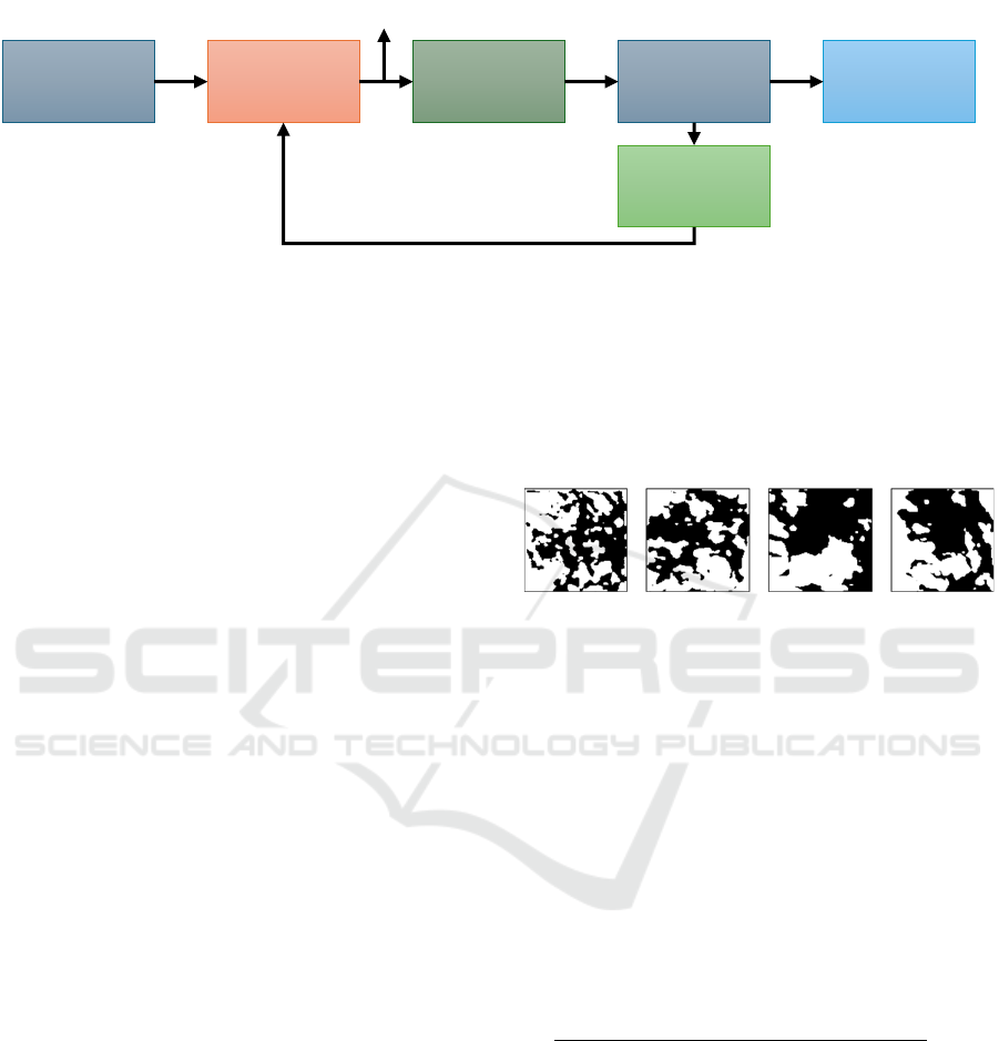
Figure 2: Flow of the segmentation algorithm adopted in this work (Kim et al., 2020). In the forward pass, the CNN processes

the input image to produce a response map. Argmax classification finds the highest probability label for each pixel. The model

then calculates loss, computes gradients, and updates parameters through the backward pass.















 









 





 



















(2)

where N is the number of pixels in the response map,

q is the number of cluster labels for each pixel in the

response map, and δ is a function of t, where δ(t) is

represented by the following equation (Kim et al.,

2020):











 

 

(3)

For the continuity constraint, L1 loss, also known

as the mean absolute error (MAE) loss, is used by the

algorithm. The L1 loss equation is as follows (Kim et

al., 2020):



















  





 















 





 







(4)

For Equation 4, W and H are the width and height

of the input image, and 





is the pixel value at (ε,η)

in the response map 





. The equation is applied for

the vertical and the horizontal components of the

input image.

Following the computation of the loss function, a

backward pass is initiated to compute gradients of the

loss with respect to the model's weights and biases.

The algorithm also makes use of a Stochastic

Gradient Descent (SGD) optimizer to update the

CNN parameters based on the computed gradients,

and the original image is passed through the CNN—

now with newly updated parameters—once again.

The whole process repeats until either the maximum

number of iterations (1000 by default) is reached, or

the CNN reaches convergence at the minimum

number of labels (set to 2). Samples of the resulting

segmentation masks are shown in Figure 3.

Figure 3: Segmentation results of the ROI samples shown

in Figure 1.

2.4 Breast Density Estimation

For the task of breast density estimation, continuous

percentage density estimates can be computed given

the segmented image masks using arithmetic division.

In essence, the segmented image is a binary image

with two regions (clusters). One of those regions is

dense, and the other is fatty. To calculate the

percentage density, the number of pixels in the dense

region is counted, divided by the total number of

pixels in the image, and multiplied by 100.

Mathematically, the equation is as follows:

  

 

(5)

The resultant density estimates are quantitative,

and can be discretized to represent qualitative labels.

To do this, a threshold is calculated based on the mean

density and the standard deviation across all images

in the dataset. Applying this threshold, the result is a

list of qualitative density labels, each pertaining to a

particular image. The qualitative labels produced in

this process are utilized in the clustering quality

evaluation described in Section 2.5 below.

CNN

Input

Image

Argmax

Classification

Cluster Labels

Loss

Calculation

Back Propagation

Segmented

Image

Response Map

VISAPP 2025 - 20th International Conference on Computer Vision Theory and Applications

694

2.5 Performance Evaluation

The evaluation process for this work comprises two

steps: an evaluation of the segmentation quality at the

pixel level and an assessment of the unsupervised

clustering quality at the per-image level. The metrics

used here are as follows: the silhouette coefficient

(SC), which measures cohesion and separation among

clusters using the following equation:

  





(6)

where A is the mean distance between a sample and

all other points in the same cluster, and B is the mean

distance between a sample and all other points in the

nearest cluster to which the sample does not belong;

the Within-Cluster Sum of Squares (WCSS), which

quantifies the compactness of clusters using the

following equation:

 



 

















(7)

where k is the number of clusters, C

is the i

cluster,

x is a data point in the cluster, u

is the centroid of the

cluster, and “||” denotes the Euclidean norm; the

Davies-Bouldin (DB) score, which assesses average

similarity between clusters using the following

equation:





 









 















(8)

where k is the number of clusters, S

is the average

distance between data points in cluster i and the

centroid of cluster i, with Sj being the cluster j

equivalent, and D

is the distance between the

centroids of clusters i and j; and the Calinski-

Harabasz (CH) index, which evaluates the ratio of

between-cluster variance to within-cluster variance

using the following equation:







  

 



(9)

where B is the between-cluster variance, W is the

within-cluster variance, N is the total number of data

points, and k is the number of clusters. To facilitate

the evaluation of the framework’s clustering ability at

the per-image level, nine features are extracted from

the images: mean luminance, standard deviation,

entropy, intensity ranges, 25

, 50

, and 75

percentiles, skewness, and kurtosis.

3 RESULTS

This section presents and discusses the results

following the evaluation of the framework described

in this work. First, an evaluation of the segmentation

is provided. Then, an evaluation of the framework’s

unsupervised labeling ability is presented. Lastly, a

discussion of the results is presented.

3.1 Segmentation Evaluation

The quality of the segmentation is evaluated at the

pixel level through the use of four metrics: SC,

WCSS, DB, and CH. This evaluation is performed

separately for the CC and MLO subsets of the dataset.

The results are shown in Table 1.

Table 1: Segmentation evaluation for CC and MLO subsets

of the INbreast dataset.

Metric\Subset

MLO

0.9491

0.9505

WCSS

3,224,218.76

2,908,076.60

0.0725

0.0697

19,471.41

13,613.63

The SC Scores average around 0.9491 for the CC

subset and range from 0.8974 to 0.9907, suggesting

notable cluster separation throughout. The WCSS

evaluation reveals an average of 3,224,218.76, with a

range between 150,933.91 and 14,200,223.75. DB

Scores have an average of 0.0725 for the CC subset,

and range from 0.0119 to 0.1813, suggesting

generally well-defined clusters. The CH Indices have

an average of 19,471.41, and range between 6.87 and

896,492.27.

In the MLO subset, SC Scores demonstrate an

average of 0.9505, and range between 0.8851 and

0.9929, showing effective segmentation. The WCSS

scores for the MLO subset have an average of

2,908,076.60, and a range from 98,592.53 to

12,226,390.39. DB Scores present an average value

of 0.0697, and a range between 0.0096 and 0.1391,

implying robust segmentation overall. The CH

Indices yield an average index value of 13,613.63,

and a range between 0.60 and 42,226.4.

Breast Density Estimation in Mammograms Using Unsupervised Image Segmentation

695

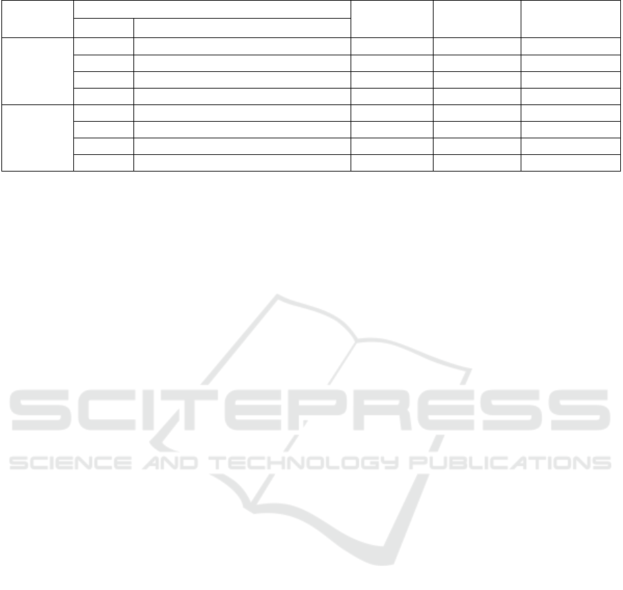
Table 2: Clustering quality evaluation for CC and MLO subsets of the INbreast dataset using a varying number of features.

Subset

Features

Silhouette

Davies-

Bouldin

Calinski-

Harabasz

Number

Set

Percentile

0.9101

0.2519

1383.58

Percentile, Luminance

0.8698

0.3245

762.69

and 50

Percentiles, Luminance

0.8469

0.3795

549.74

All

0.6238

0.6889

104.15

MLO

Kurtosis

0.9416

0.0787

1806.60

Skewness, Kurtosis

0.9036

0.128

1016.62

Skewness, Kurtosis, 50

Percentile

0.8437

0.2260

772.06

All

0.5977

0.6373

199.47

3.2 Clustering Quality Evaluation

In this section, the clustering quality, or the quality of

the unsupervised labeling of images as fatty or dense,

is evaluated. This is done with metrics that do not rely

on ground truth, and instead measure the quality of

and separation between clusters: the SC, the DB

Score, and the CH Index. The metrics were computed

separately for CC and MLO images based on

extracted statistical features—mean luminance,

standard deviation, statistical entropy, pixel intensity

ranges (the maximum minus the minimum for each

image), the 25th, 50th, and 75th percentiles,

skewness, and kurtosis—after MinMax scaling. The

results are shown in Table 2. In the context of breast

density estimation, the SC indicates well-defined

density categories, the CH index shows the

distinctness and compactness of clusters, and the DB

score measures the separation and cohesion of these

clusters. Higher SC and CH values and a lower DB

score indicate better clustering quality.

Combining all features, the resulting SC score for

CC images was 0.6238, which indicates notable

cohesion and separation between clusters. The DB

score was 0.6889, and the CH Index was 104.15, both

of which suggest a reasonable degree of separation

between clusters. Using only the 25th percentile to

represent the images results in the highest SC score

(0.9101). Using mean luminance and the 25th

percentile is also representative, resulting in a SC

score of 0.8698. When using three features,

combining the mean luminance and the 25th

percentile with the 50th percentile is the most

effective for CC images, resulting in a SC score of

0.8469.

For the MLO subset of the dataset, the

combination of all features results in a SC score of

0.5977, a DB score of 0.6373, and a CH index of

199.47. This indicates a notable degree of separation

and cohesion between and among clusters. In contrast

to CC, the most representative feature for MLO is

kurtosis, and it results in a SC score of 0.9416.

Combining kurtosis with skewness results in a SC

score of 0.9036. For three features, the highest SC

score (0.8437) results from combining skewness,

kurtosis, and the 50th percentile.

3.3 Discussion

The segmentation evaluation shows strong pixel-

level performance for both CC and MLO images,

with high SC scores indicating good cluster cohesion

and separation. DB scores suggest effective

clustering, though WCSS and CH scores vary. For

unsupervised labeling of Fatty or Dense, key features

like the 25th percentile and mean luminance for CC,

and kurtosis and skewness for MLO, effectively

distinguish clusters. While adding more features

might introduce noise, combining all features still

achieves significant separation between Fatty and

Dense categories.

These results are promising and suggest that the

proposed framework can distinguish between Fatty

and Dense breasts in an unsupervised manner. This is

a non-subjective approach as it does not rely on expert

assessment. In contrast, the current state-of-the-art

methods exclusively rely on expert-assigned labels

for classification and hand-annotated markings for

segmentation. Additionally, the framework is highly

generalizable, given that it does not need to be trained

on a specific dataset, and it is also highly adaptable.

Furthermore, it is inexpensive and fully automatic,

which means that it is easily integrable into clinical

settings.

The novelty of this work lies in the

implementation of unsupervised image segmentation

to solve the problem of breast density estimation,

which has not been done before. Though the

segmentation algorithm is directly adopted with

limited changes, it is extensively tuned for the task

and integrated into a task-specific, scalable

framework, with automated image selection, breast

VISAPP 2025 - 20th International Conference on Computer Vision Theory and Applications

696

reorientation, artifact removal, ROI extraction, and

continuous and binary density estimation modules.

Numerical comparison of the results to other works in

the literature is not possible at this stage, as they

exclusively employ traditional classification metrics.

In the future, the agreement between the expert labels

and the framework’s binary labels will be measured,

enabling comparison to other works through

classification metrics.

4 CONCLUSION

This work introduced a framework for breast density

estimation through unsupervised segmentation of

mammographic images. It includes preprocessing

methods for breast reorientation, artifact and noise

removal, and ROI extraction. A state-of-the-art

segmentation algorithm was tuned for breast density

segmentation, and percentage density estimation was

performed using an arithmetic division approach.

Breast density was then discretized into two classes,

Fatty and Dense, via a thresholding approach. The

framework’s segmentation quality and unsupervised

labeling ability were evaluated, showing robust

performance. For segmentation at the pixel-level,

silhouette scores averaging 0.95 were achieved.

Further, for the unsupervised labeling of

mammograms, an average silhouette score of 0.61

was attained. This suggests the framework’s potential

as a support tool for radiologists in a clinical setting.

For future work, the framework’s agreement with

expert labels will be evaluated. Further, other datasets

will be used to test and verify the generalizability of

the framework. In addition, supplemental testing will

be conducted to determine if the framework can be

further refined, such as through the use of ROIs with

adaptive sizes rather than fixed sizes, or through the

employment of other unsupervised segmentation

algorithms. Moreover, to improve the error-handling

ability of the framework, a postprocessing procedure

will be implemented to reassign labels to incorrectly

classified images through the use of a confidence

metric.

REFERENCES

Arefan, D., Talebpour, A., Ahmadinejhad, N., & Asl, A. K.

(2015). Automatic breast density classification using

neural network. Journal of Instrumentation, 10(12).

https://doi.org/10.1088/1748-0221/10/12/T12002

Birdwell, R. L. (2009). The preponderance of evidence

supports computer-aided detection for screening

mammography. In Radiology (Vol. 253, Issue 1).

https://doi.org/10.1148/radiol.2531090611

Byng, J. W., Boyd, N. F., Fishell, E., Jong, R. A., & Yaffe,

M. J. (1994). The quantitative analysis of

mammographic densities. Physics in Medicine and

Biology, 39(10). https://doi.org/10.1088/0031-

9155/39/10/008

Dehghani, S., & Dezfooli, M. A. (2011). A Method For

Improve Preprocessing Images Mammography.

International Journal of Information and Education

Technology. https://doi.org/10.7763/ijiet.2011.v1.15

Dhou, S., Alhusari, K., & Alkhodari, M. (2024). Artificial

intelligence in mammography: advances and

challenges. In Artificial Intelligence and Image

Processing in Medical Imaging (pp. 83–114). Elsevier.

https://doi.org/10.1016/B978-0-323-95462-4.00004-2

Dhou, S., Dalah, E., AlGhafeer, R., Hamidu, A., &

Obaideen, A. (2022). Regression Analysis between the

Different Breast Dose Quantities Reported in Digital

Mammography and Patient Age, Breast Thickness, and

Acquisition Parameters. Journal of Imaging, 8(8), 211.

https://doi.org/10.3390/jimaging8080211

Gram, I. T., Funkhouser, E., & Tabár, L. (1997). The Tabar

classification of mammographic parenchymal patterns.

European Journal of Radiology, 24(2).

https://doi.org/10.1016/S0720-048X(96)01138-2

Gudhe, N. R., Behravan, H., Sudah, M., Okuma, H.,

Vanninen, R., Kosma, V. M., & Mannermaa, A. (2022).

Area-based breast percentage density estimation in

mammograms using weight-adaptive multitask

learning. Scientific Reports, 12(1).

https://doi.org/10.1038/s41598-022-16141-2

Hartman, K., Highnam, R., Warren, R., & Jackson, V.

(2008). Volumetric assessment of breast tissue

composition from FFDM images. Lecture Notes in

Computer Science (Including Subseries Lecture Notes

in Artificial Intelligence and Lecture Notes in

Bioinformatics), 5116 LNCS.

https://doi.org/10.1007/978-3-540-70538-3_5

Kallenberg, M., Petersen, K., Nielsen, M., Ng, A. Y., Diao,

P., Igel, C., Vachon, C. M., Holland, K., Winkel, R. R.,

Karssemeijer, N., & Lillholm, M. (2016). Unsupervised

Deep Learning Applied to Breast Density Segmentation

and Mammographic Risk Scoring. IEEE Transactions

on Medical Imaging, 35(5).

https://doi.org/10.1109/TMI.2016.2532122

Kim, W., Kanezaki, A., & Tanaka, M. (2020).

Unsupervised Learning of Image Segmentation Based

on Differentiable Feature Clustering. IEEE

Transactions on Image Processing, 29.

https://doi.org/10.1109/TIP.2020.3011269

Li, H., Giger, M. L., Huo, Z., Olopade, O. I., Lan, L.,

Weber, B. L., & Bonta, I. (2004). Computerized

analysis of mammographic parenchymal patterns for

assessing breast cancer risk: Effect of ROI size and

location. Medical Physics, 31(3).

https://doi.org/10.1118/1.1644514

Moreira, I. C., Amaral, I., Domingues, I., Cardoso, A.,

Cardoso, M. J., & Cardoso, J. S. (2012). INbreast:

Toward a Full-field Digital Mammographic Database.

Breast Density Estimation in Mammograms Using Unsupervised Image Segmentation

697

Academic Radiology, 19(2).

https://doi.org/10.1016/j.acra.2011.09.014

Nahler, G. (2009). visual analogue scale (VAS). In

Dictionary of Pharmaceutical Medicine.

https://doi.org/10.1007/978-3-211-89836-9_1450

Nazari, S. S., & Mukherjee, P. (2018). An overview of

mammographic density and its association with breast

cancer. In Breast Cancer (Vol. 25, Issue 3).

https://doi.org/10.1007/s12282-018-0857-5

Saffari, N., Rashwan, H. A., Abdel-Nasser, M., Singh, V.

K., Arenas, M., Mangina, E., Herrera, B., & Puig, D.

(2020). Fully automated breast density segmentation

and classification using deep learning. Diagnostics,

10(11). https://doi.org/10.3390/diagnostics10110988

Sickles, EA, D’Orsi CJ, Bassett LW, et al. (2013). ACR BI-

RADS® Mammography. In: ACR BI-RADS® Atlas,

Breast Imaging Reporting and Data System. Reston,

VA, American College of Radiology.

Sprague, B. L., Conant, E. F., Onega, T., Garcia, M. P.,

Beaber, E. F., Herschorn, S. D., Lehman, C. D.,

Tosteson, A. N. A., Lacson, R., Schnall, M. D., Kontos,

D., Haas, J. S., Weaver, D. L., & Barlow, W. E. (2016).

Variation in Mammographic Breast Density

Assessments among Radiologists in Clinical Practice:

A Multicenter Observational Study. Annals of Internal

Medicine, 165(7). https://doi.org/10.7326/M15-2934

Sung, H., Ferlay, J., Siegel, R. L., Laversanne, M.,

Soerjomataram, I., Jemal, A., & Bray, F. (2021). Global

Cancer Statistics 2020: GLOBOCAN Estimates of

Incidence and Mortality Worldwide for 36 Cancers in

185 Countries. CA: A Cancer Journal for Clinicians,

71(3). https://doi.org/10.3322/caac.21660

Wengert, G. J., Helbich, T. H., Leithner, D., Morris, E. A.,

Baltzer, P. A. T., & Pinker, K. (2019). Multimodality

Imaging of Breast Parenchymal Density and

Correlation with Risk Assessment. In Current Breast

Cancer Reports (Vol. 11, Issue 1).

https://doi.org/10.1007/s12609-019-0302-6

Wolfe, J. N. (1976). Breast patterns as an index of risk for

developing breast cancer. American Journal of

Roentgenology, 126(6).

https://doi.org/10.2214/ajr.126.6.1130

VISAPP 2025 - 20th International Conference on Computer Vision Theory and Applications

698