Real-Time Network-Aware Roadside LiDAR Data Compression
Md Parvez Mollah
1 a
, Murugan Sankaradas
2 b
, Ravi K. Rajendran
2 c
and Srimat T. Chakradhar
2 d
1
Department of Computer Science, The University of New Mexico, Albuquerque, New Mexico, U.S.A.
2
NEC Laboratories America, Inc., Princeton, New Jersey, U.S.A.
Keywords:
Roadside LiDAR, Background Subtraction, Sensor-Agnostic Compression, Cloud, Edge Systems.
Abstract:
LiDAR technology has emerged as a pivotal tool in Intelligent Transportation Systems (ITS), providing unique
capabilities that have significantly transformed roadside traffic applications. However, this transformation
comes with a distinct challenge: the immense volume of data generated by LiDAR sensors. These sensors
produce vast amounts of data every second, which can overwhelm both private and public 5G networks that
are used to connect intersections. This data volume makes it challenging to stream raw sensor data across
multiple intersections effectively. This paper proposes an efficient real-time compression method for roadside
LiDAR data. Our approach exploits a special characteristic of roadside LiDAR data: the background points
are consistent across all frames. We detect these background points and send them to edge servers only once.
For each subsequent frame, we filter out the background points and compress only the remaining data. This
process achieves significant temporal compression by eliminating redundant background data and substantial
spatial compression by focusing only on the filtered points. Our method is sensor-agnostic, exceptionally fast,
memory-efficient, and adaptable to varying network conditions. It offers a 2.5x increase in compression rates
and improves application-level accuracy by 40% compared to current state-of-the-art methods.
1 INTRODUCTION
The advent of Intelligent Transportation Systems
(ITS) has ushered in a new era of innovation and ef-
ficiency in managing our road networks. At the heart
of this transformation lies the need for real-time, ac-
curate, and comprehensive data that empowers traf-
fic authorities to make informed decisions, enhances
road safety, and eases the daily commute for mil-
lions of travelers. In this context, Light Detection
and Ranging (LiDAR) technology has emerged as a
pivotal tool, offering unique capabilities that have re-
shaped the landscape of roadside traffic applications.
Unlike conventional camera-based systems, Li-
DAR sensors provide a dynamic and precise un-
derstanding of traffic dynamics and road condi-
tions. Their ability to capture high-resolution, three-
dimensional data equips them to excel in applications
such as traffic monitoring, congestion management,
pedestrian safety, and infrastructure assessment. The
advantages of LiDAR over cameras are evident. For
a
https://orcid.org/0000-0002-7131-1354
b
https://orcid.org/0000-0002-4608-1630
c
https://orcid.org/0009-0002-3663-8869
d
https://orcid.org/0000-0003-3530-3901
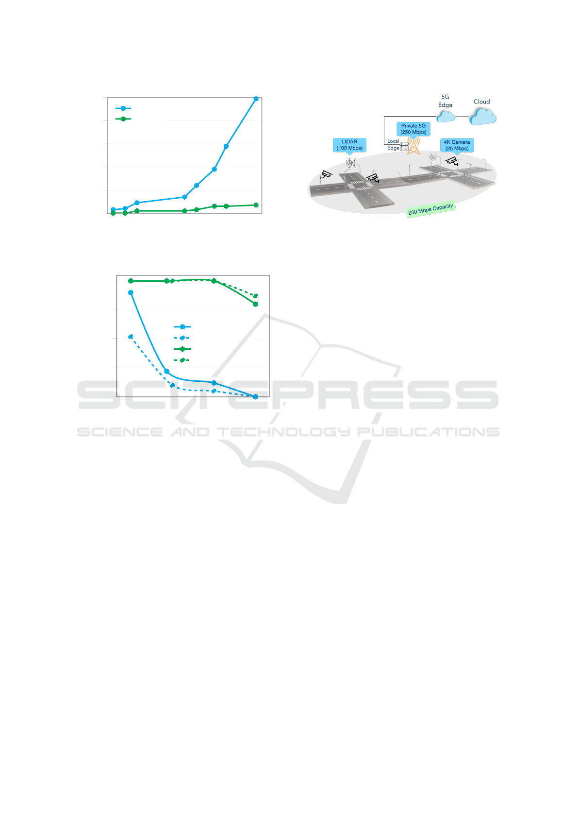
instance, as illustrated in Figure 1, 3D reconstruc-
tion errors for cameras increase as the distance grows
(Li and Yoon, 2023). Additionally, cameras ex-
hibit reduced performance in low light, particularly
at night, where their effectiveness diminishes by ap-
proximately 20% for every meter (refer to Figure 2).
In contrast, LiDAR operates independently of ambi-
ent light, ensuring reliability both day and night, and
possesses depth perception capabilities that facilitate
precise object detection and tracking even in complex,
cluttered environments. Consequently, LiDAR proves
better suited for roadside traffic applications.
Private 5G networks are proposed in traffic inter-
section applications by operators to interconnect in-
tersections, because they offer high bandwidth, low
latency, security, and control. The context to deploy
LiDARs at traffic intersections and connect them with
private 5G networks to transmit the data to the cloud,
enabling real-time analytics for roadside traffic appli-
cations (as shown in Figure 3). LiDAR is a promising
technology for traffic applications, but its high data
volume is a challenge. Private 5G cannot stream raw
data from sensors across multiple intersections. This
challenge underscores the pressing need for the de-
velopment of efficient data compression methods tai-
136
Mollah, M. P., Sankaradas, M., Rajendran, R. K. and Chakradhar, S. T.
Real-Time Network-Aware Roadside LiDAR Data Compression.
DOI: 10.5220/0013298900003941
Paper published under CC license (CC BY-NC-ND 4.0)
In Proceedings of the 11th International Conference on Vehicle Technology and Intelligent Transport Systems (VEHITS 2025), pages 136-147
ISBN: 978-989-758-745-0; ISSN: 2184-495X
Proceedings Copyright © 2025 by SCITEPRESS – Science and Technology Publications, Lda.

0
5
10
15
20
25
0
1
2
3
4
5
Distance (in meters)
3D Reconstruction error
(in meters)
Camera
LiDAR
Figure 1: 3-D reconstruction error comparison for cameras
and LiDARs (Li and Yoon, 2023).
10 20 30 40
50 60
0
25
50
75
100
Distance to stop bar (in meters)
Vechicle Detection Accuracy (%)
Camera-at-day
Camera-at-night
LiDAR-at-day
LiDAR-at-night
Figure 2: Camera vs LiDAR performance comparison in
different lighting condition (Guan et al., 2023).
lored specifically to roadside LiDAR data.
To develop such a technique, we need to address
three challenges. First, the compression method must
be capable of running on low-cost computing devices
to reduce installation costs. Second, the compression
must be sensor-agnostic, meaning it should work with
different types of LiDAR scanning patterns. It should
also be network-aware to handle fluctuating network
speeds, as the network will be shared among many
devices. Third, LiDAR data must be made available
in real-time at the edge or in the cloud for processing
and further analytics.
In this paper, we develop an efficient real-time
compression method by exploiting a unique char-
acteristic of roadside LiDAR data: the background
points in roadside LiDARs are repeated across all
frames. Our idea is to detect and send the back-
ground points to the cloud only once. Subsequently,
we filter the background points for each frame and
only compress the filtered frames. By filtering the
backgrounds, our method achieves substantial tempo-
Figure 3: Deployment of LiDAR sensors at the traffic inter-
sections and connecting them with shared private 5G net-
work.
ral compression, and by compressing only the filtered
points, it gains significant spatial compression as well.
Our key contributions of this paper are as follows:
• We propose a novel compression scheme for road-
side LiDAR data that filters out background points
from frames before compression, as these points
are unnecessary for downstream applications.
• We propose an extremely fast and memory effi-
cient background detection and filtering technique
that can be used with other existing point cloud
compression methods to increase their efficiency.
• We develop a sensor-agnostic, real-time network-
aware point cloud compression mechanism for
roadside LiDARs. To the best of our knowledge,
this is the first work that can adapt compression
rate based on the available network bandwidth.
• Our compression system achieves 2.5x higher
compression rates with faster compression speeds
and minimal reconstruction errors compared to
state-of-the-art compression methods. Moreover,
our method achieves higher application-level ac-
curacy compared to the best alternative.
2 RELATED WORK
2.1 Background Detection and Filtering
The task of background detection and filtering from
the roadside LiDAR data has been widely explored in
recent years. Most of the works in literature can be
categorized into two groups based on the methodol-
ogy used: i) density-based (Wu et al., 2018; Lv et al.,
2019; Lin et al., 2023) ii) feature-based (Zhao et al.,
2019; Zhao et al., 2023).
Density-based methods divide the entire 3-D
space into smaller cubes and compute the point den-
Real-Time Network-Aware Roadside LiDAR Data Compression
137

sity of each cube for a certain amount of time. The
idea is that the density of background points will be
higher than moving object points for static LiDARs.
To find a density threshold to separate the background
points, (Wu et al., 2018) uses the density value where
the slope of the frequency curve of the point densi-
ties becomes positive. In (Lin et al., 2023), the au-
thors perform several steps such as identifying road
user passing area, removing outliers using DBSCAN
algorithm, etc., on top of computing density of cubes.
The main limitation of density-based methods is that
working in 3D space require huge amount of memory,
which is not feasible to deploy in low-cost computa-
tion units on traffic poles.
Feature-based methods exploit the characteristics
of the point cloud data to identify the background
points. For example, (Zhao et al., 2019) detects
and filters the background points by comparing the
heights between raw LiDAR data and background ob-
jects based on laser channels and azimuth angles. In
(Zhao et al., 2023), a 2D channel-azimuth background
table is generated by learning the critical distance in-
formation of both static and dynamic backgrounds.
Feature-based methods do not suffer from memory in-
efficiency, however, they require 100 −300 millisec-
onds to filter backgrounds from a frame, which is ex-
pensive for our case.
Existing works treat background detection and fil-
tering as a single task. For them, a few gigabytes
of memory or a few hundred milliseconds of time
suffice. However, in our case, background detection
must be memory-efficient, as it will operate on low-
cost devices. Furthermore, background filtering must
be exceptionally fast, as we need to run the compres-
sion mechanism on top of it.
2.2 Compression
Various compression methods have been proposed in
literature for point cloud data. The most used method
for encoding point cloud data typically involves the
utilization of space-partitioning trees, with Octree be-
ing the predominant choice (Golla and Klein, 2015;
Lasserre et al., 2019; Thanou et al., 2016). The
G-PCC technique, a part of the MPEG point cloud
compression standard, also falls within this category
(Lasserre et al., 2019). Each leaf node of the Oc-
tree can be encoded using either a single occupancy
bit, which can be lossless when each leaf node con-
tains precisely one point, or through plane extraction,
which preserves more intricate details when multi-
ple points reside within a leaf node. G-PCC offers
both of these encoding options. Building upon the
foundation of space-partitioning tree representation,
prior research has explored diverse strategies to mit-
igate redundant information, such as employing mo-
tion compensation in 3D space (Thanou et al., 2016),
or directly applying video compression techniques
(Golla and Klein, 2015). Google also develops a
generalized method for compressing 3-D meshes and
point clouds (Google, 2018). While these approaches
prove effective in specific use cases, one drawback
of unstructured representations is their failure to ex-
ploit the distinctive characteristics exposed by LiDAR
point clouds, resulting in generally lower compres-
sion rates.
Another family of works convert point clouds into
2-D images using spherical projection (Sun et al.,
2019; Tu et al., 2019) or orthogonal projection (Kri-
voku
´
ca et al., 2020) and then use existing image/video
compression methods to compress the projected im-
ages. Due to applying image and video compression
algorithms, these methods fail to retain the inherent
spatial information within the point cloud, which typ-
ically leads to reduced accuracy in down-the-pipeline
applications.
Some recent works focus on specific use cases
of LiDARs and develop compression techniques only
suitable for those use cases (Feng et al., 2020; Mol-
lah et al., 2022). For example, (Feng et al., 2020)
compresses point cloud data from moving LiDARs
by using coordinate transformation and 3-D plane fit-
ting, whereas (Mollah et al., 2022) proposes a batch
compression technique for roadside LiDARs by using
wavelet decomposition to capture quick transition of
vehicles.
Since our goal is to enable massive device con-
nectivity and stream data in real-time, we need a
compression mechanism with strict bandwidth and la-
tency requirements. None of the existing methods are
suitable for our case as they fail to meet either the
bandwidth or the latency requirements while keeping
down-the-pipeline application accuracy.
3 PROPOSED SYSTEM
3.1 System Architecture
In this section, we provide a brief overview of our
proposed system. Figure 4 illustrates a block diagram
of how the components of our system interact with
each other. Our system comprises two primary com-
ponents: i) the Background Extraction Module, and
ii) the Compression Module.
The task of the Background Extraction Module is
to identify background points by analyzing a set of
raw LiDAR frames. To accomplish this, it computes
VEHITS 2025 - 11th International Conference on Vehicle Technology and Intelligent Transport Systems
138

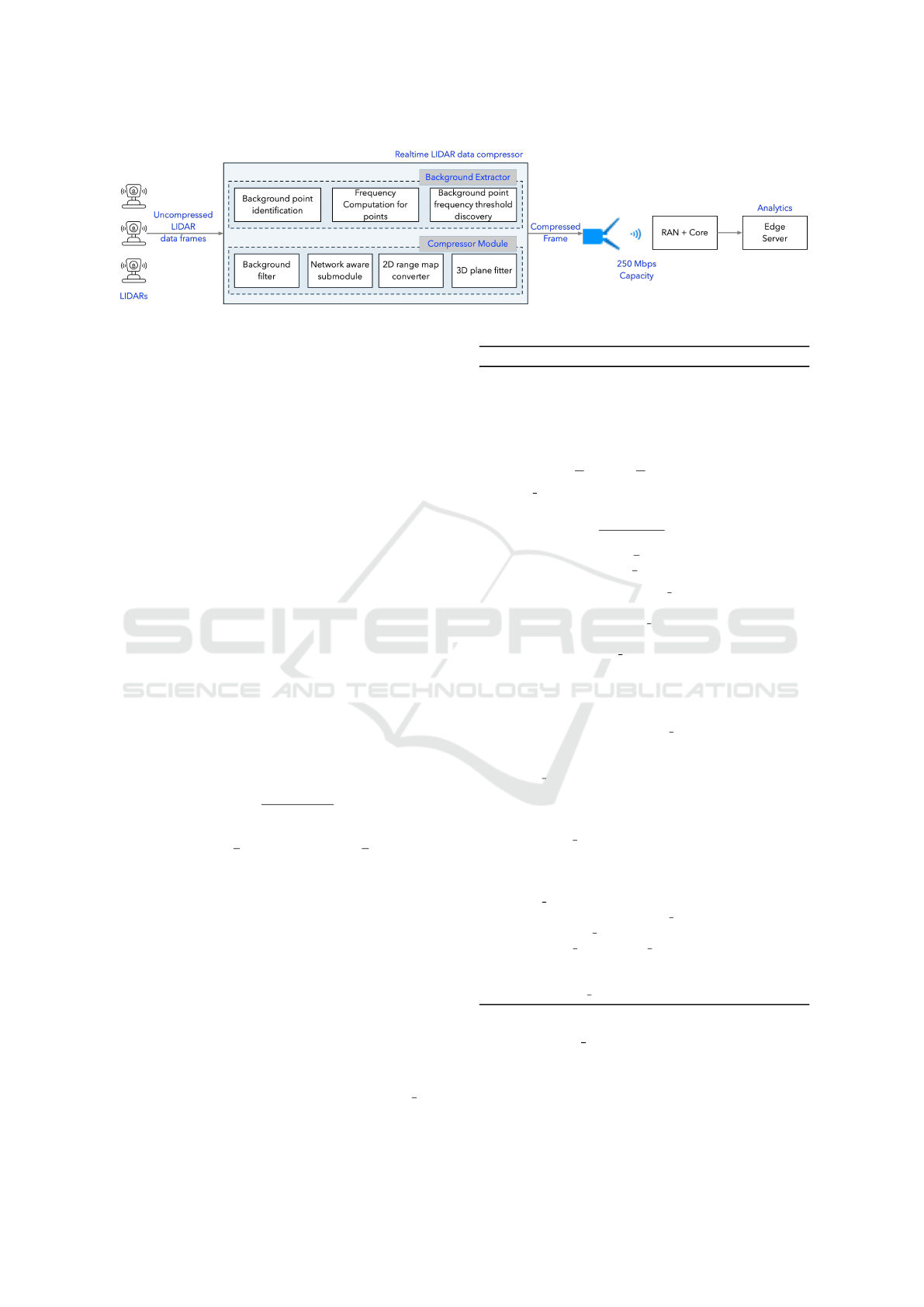
Figure 4: Block diagram of our proposed compression system.
the frequency of each point across the set of frames
and determines a frequency threshold to separate the
background points. Once the background points are
identified, they are stored within the system for use
by the Compression Module.
The Compression Module, on the other hand,
takes a raw LiDAR frame, filters out the background,
and then determines the size of the range map using
the network-aware sub-module. Subsequently, the fil-
tered frame is converted into a range map, and a 3-D
plane fitting method is applied to compress the frame.
The compressed frame is then transmitted to the edge
via the 5G network for real-time analytics.
3.2 Background Detection and Filtering
The key idea of our background detection and filter-
ing techniques involves transforming the 3-D point
cloud frame into a 2-D grid, referred to as a range
map, through spherical projection. This conversion
serves the purpose of grouping the 3-D points into
discrete buckets, enabling the counting of their fre-
quencies across all frames.
To convert each point (x,y,z) of a point cloud
frame to a value r at index (φ,θ) in the range map:
r =
p
x
2
+ y
2
+ z
2
, (1)
φ = ⌊arccos(
z
r
)/φ
l
⌋,θ = ⌊arctan(
x
y
)/θ
l
⌋, (2)
where φ
l
and θ
l
are the vertical and horizontal resolu-
tions of the LiDAR, respectively.
Algorithm 1 describes how our background detec-
tion works. The algorithm takes a stream of point
cloud frames P (usually 5 minutes of frames), ver-
tical and horizontal resolutions of LiDAR φ
l
and θ
l
,
LiDAR’s vertical and horizontal field of view V and
H, and a nearest neighbor distance threshold D
t
as
inputs and outputs a set of 3-D points which are iden-
tified as background points. The algorithm works as
follows:
At first, the dimensions of the range map are com-
puted (line 1), and an empty 2-D range map r map
with the computed dimensions is initialized (line 2).
Algorithm 1: Background Detection Algorithm.
Require: A set of point cloud frames P with n frames,
LiDAR vertical resolution φ
l
, LiDAR horizontal
resolution θ
l
, LiDAR V-FoV V , LiDAR H-FoV H,
nearest neighbor distance threshold D
t
Ensure: A set of (x, y,z) points, which are detected as
background points
1: rows ←
V
φ
l
,cols ←
H
θ
l
2: r map(1 : rows,1 : cols) ←
/
0
3: for each frame p ∈ P do
4: for each point (x,y,z) ∈ p do
5: d ←
p
x
2
+ y
2
+ z
2
6: r ← ⌊arccos (
z
d
)/φ
l
⌋
7: c ← ⌊arctan (
x
y
)/θ
l
⌋
8: (x
n
,y
n
,z
n
) ← NN(r map(r,c),(x, y,z), D
t
)
9: if (x
n
,y
n
,z
n
) ̸=
/
0 then
10: updateFrq(r map(r,c),(x
n
,y
n
,z
n
))
11: else
12: insert(r map(r,c),(x,y,z,1))
13: end if
14: end for
15: end for
16: f r ←
/
0
17: for for each (x,y,z, c) ∈ r map do
18: f r(c) ← f r(c) + 1
19: end for
20: f r threshold ← 0
21: keys ← getMapKeys( f r)
22: for i ← 2 : length(keys) do
23: if f r(keys(i))− f r(keys(i −1)) then
24: f r thresold ←keys(i)
25: break
26: end if
27: end for
28: bg points ←
/
0
29: for for each (x,y,z, c) ∈ r map do
30: if c ≥ f r threshold then
31: bg points ← bg points ∪{(x,y,z)}
32: end if
33: end for
34: return bg points
Each index of r map contains a kd-tree where each
leaf of the kd-tree takes a 4-tuple value (x, y,z,c),
where (x,y, z) represents the 3-D coordinates of the
projected point, and c is the frequency of that point
across all frames. Then, the algorithm processes each
Real-Time Network-Aware Roadside LiDAR Data Compression
139

(x,y, z) point from every point cloud frame p in P and
computes its index (r,c) in r map using the spherical
projection described in Eq. 1 and 2 (lines 3-7). In line
8, the algorithm finds the nearest neighbor of (x,y,z)
by performing a query in the kd-tree at index (r, c) of
r map. If a nearest neighbor is found within the given
distance threshold D
t
, the algorithm updates the fre-
quency of that nearest neighbor in the kd-tree (lines
9-10). Otherwise, the algorithm inserts a new 4-tuple
value (x, y,z,1) into the kd-tree (lines 11-13) to indi-
cate that this (x,y,z) point has not been observed in
any previous frames.
Next, the algorithm computes the frequency
threshold and separates the background points based
on that threshold (lines 16-34). To do so, an empty
map f r is initialized (line 16), where the key rep-
resents the frequency of the (x , y,z) points across
all frames, and the value indicates how many times
that frequency occurs in the r map. The algorithm
then iterates through each tuple (x,y,z,c) from the
r map and increments the frequency count for c in
the map f r (lines 17-19). Subsequently, the fre-
quency threshold f r threshold is computed by ana-
lyzing the key-value pairs of the map f r and iden-
tifying the point where the slope of the frequency
curve of point frequencies becomes positive (lines 20-
27). Finally, in lines 28-34, the algorithm marks the
(x,y, z) points with a frequency greater than or equal
to f r threshold as background points, stores them in
the set bg points, and returns the set.
Once the background points are identified, filter-
ing them from a point cloud frame p is a straightfor-
ward process. Algorithm 2 describes the filtering pro-
cedure. The algorithm takes a point cloud frame p,
from which the background points need to be filtered,
a set of (x,y,z) points bg points identified as back-
grounds points, LiDAR vertical resolution φ
l
, LiDAR
horizontal resolution θ
l
, LiDAR vertical field of view
V , LiDAR horizontal field of view H, and a nearest
neighbor distance threshold D
t
and outputs a set of
non-background (x, y,z) points. The algorithm works
as follows:
Initially, the background points are transformed
into 2-D space using the same spherical projection
method as described in Algorithm 1, and they are
stored in the range map r map (lines 1-8). Sub-
sequently, for each point (x,y, z) in the point cloud
frame p, the algorithm computes its spherical pro-
jection (r,c) and searches for the nearest neighbor in
the kd-tree indexed at (r, c) in r map (lines 9-14). If
no nearest neighbor is found within the specified dis-
tance threshold D
t
, the point (x,y, z) is classified as
a non-background point (lines 15-17). Consequently,
the algorithm adds it to the set nonbg points (line 16).
Algorithm 2: Background Filtering Algorithm.
Require: a point cloud frame p, a set of (x, y,z) points
bg points, LiDAR vertical resolution φ
l
, LiDAR
horizontal resolution θ
l
, LiDAR V-FoV V , LiDAR
H-FoV H, nearest neighbor distance threshold D
t
Ensure: A set of (x, y,z) points, which are kept as
non-background points.
1: rows ←
V
φ
l
,cols ←
H
θ
l
2: r map(1 : rows,1 : cols) ←
/
0
3: for each point (x,y,z) ∈ bg points do
4: d ←
p
x
2
+ y
2
+ z
2
5: r ← ⌊arccos (
z
d
)/φ
l
⌋
6: c ← ⌊arctan (
x
y
)/θ
l
⌋
7: insert(r map(r,c),(x,y,z))
8: end for
9: nonbg points ←
/
0
10: for each point (x,y,z) ∈ p do
11: d ←
p
x
2
+ y
2
+ z
2
12: r ← ⌊arccos (
z
d
)/φ
l
⌋
13: c ← ⌊arctan (
x
y
)/θ
l
⌋
14: (x
n
,y
n
,z
n
) ← NN(r map(r,c),(x, y,z), D
t
)
15: if (x
n
,y
n
,z
n
) =
/
0 then
16: nonbg points ← nonbg points ∪{(x,y,z)}
17: end if
18: end for
19: return nonbg points
After processing all points in frame p, the algorithm
returns the set nonbg points as the output (line 19).
3.3 Network-Aware Compression
Background filtering achieves significant temporal
compression (discussed in Section 4.5) by removing
repeated background points across multiple frames.
To further reduce the size of the data, we perform
spatial compression on the filtered point cloud frames
by using 3-D plane fitting method. Since most of the
real-world surfaces are 3-D planes e.g., sides of cars,
ground, etc., all points that lie on the same plane can
be encoded by using that plane. We can also approxi-
mate non-plane surfaces by using a set of planes.
As discussed in (Feng et al., 2020), a plane in 3-D
Cartesian space can be represented as:
x + ay + bz −c = 0, (3)
where (1,a,b) is the normal vector of the plane and
|c|
√
1+a
2
+b
2
is the distance from the origin i.e., center
of the LiDAR. Hence, we can encode all points on the
same plane with just three coefficients. Since the ex-
act position of each point on the plane is not explicitly
encoded, we need to perform a ray casting process to
find the intersection of a ray and the plane to recon-
struct the position of a point.
VEHITS 2025 - 11th International Conference on Vehicle Technology and Intelligent Transport Systems
140

To find the points that may lie on the same plane,
we utilize the range map conversion of the point
cloud. As adjacent grids in the range map correspond
to consecutive scans from the LiDAR, the points
mapped to them are likely to lie on the same plane.
We initially partition the range map into uniform unit
sub-grids, for example, 4 × 4 in size. The process be-
gins with fitting a plane to the points within the first
sub-grid and progressively extends to fit neighboring
sub-grids, effectively creating a larger sub-grid. Dur-
ing each expansion step, we evaluate whether the cur-
rent plane fitting can satisfactorily represent all the
points within the newly enlarged sub-grid, adhering
to a predefined threshold. If the criteria are met, all
the points in the expanded sub-grid are encoded using
the same plane coefficients. In cases where the crite-
ria are not met, we restart the process from the cur-
rent sub-grid and continue until all sub-grids within
the range map have been processed.
Expressing the task of fitting a plane to a set of
points can be naturally framed as a linear least squares
problem (Nievergelt, 1994). Although traditional iter-
ative approaches like RANSAC (Fischler and Bolles,
1981) are commonly employed, we use closed-form
solution as suggested by (Feng et al., 2020) because
it requires less computation and the computations can
be parallelized.
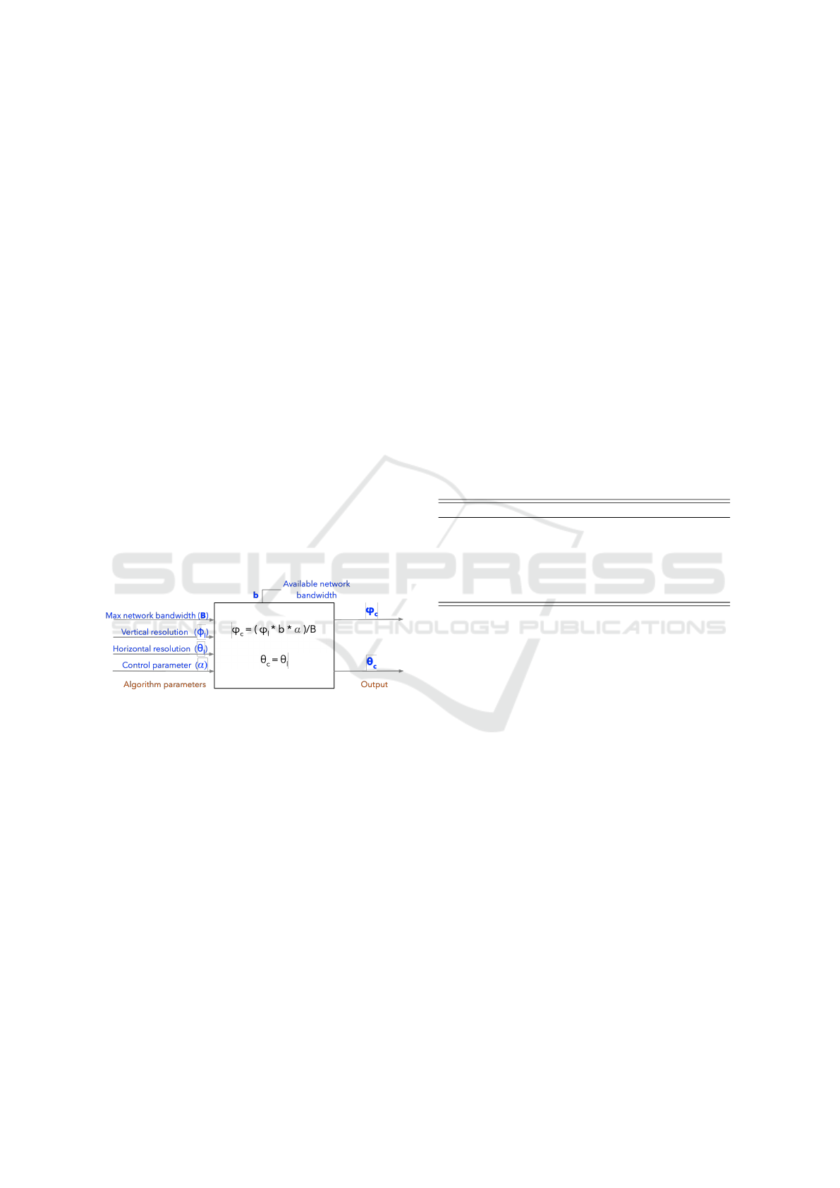
Figure 5: Network-aware module to adapt compression rate
with available network bandwidth.
Finally, to make the compression network-aware,
we vary the size of the range map according to the
available network bandwidth while converting from
the filtered point cloud frame. The idea is that a
smaller range map would yield a higher compression
rate and vice versa. Recall that, the dimensions of
the range map depend on the vertical and horizontal
resolutions of the LiDAR, denoted as φ
l
and θ
l
, re-
spectively. We introduce two parameters φ
c
and θ
c
,
initially set as φ
l
and θ
l
, respectively. Subsequently,
we modify these parameters to change the dimensions
of the range map, thereby enabling us to regulate the
compression rate (see Figure 5). How to effectively
tune these parameters in response to the available net-
work bandwidth is detailed in Section 4.7.
4 EXPERIMENTAL EVALUATION
In this section, we provide a comprehensive empirical
assessment of the proposed technique using several
real-world datasets, comparing its performance with
various baseline methods.
4.1 Evaluation Setup
We employ LiDAR sensors from three different ven-
dors in our evaluation: Neuvition Titan M1, Livox
Mid-70, and Ouster OS-1. This choice allows us to
demonstrate the sensor-agnostic nature of our com-
pression method. Neuvition and Ouster LiDARs ex-
hibit repetitive scanning patterns, whereas the Livox
LiDAR employs a non-repetitive scanning pattern. A
summary of the sensor configurations that include the
horizontal field of view (H-FoV), the vertical field of
view (V-FoV), the frame rate and the scan pattern is
described in Table 1.
Table 1: Sensor configurations.
Vendor H-FoV V-FoV Frame rate Scan pattern
Neuvition
Titan M1
45
◦
25
◦
10 Hz Repetitive
Livox
Mid-70
70.4
◦
70.4
◦
10 Hz Non-repetitive
Ouster
OS-1
360
◦
45
◦
10 Hz Repetitive
We connect the LiDAR to a Raspberry Pi with
Ubuntu as the edge unit and run our compression sys-
tem on it. The point cloud frames generated by the
LiDAR sensor are processed using various libraries
such as OpenCV, Boost, and PCL (Rusu and Cousins,
2011). To stream the compressed data to an edge
server, we utilize a Celona private 5G wireless setup.
4.2 Evaluation Datasets
We have collected three real-world datasets (NEC-
Neuvition, NEC-Livox, NEC-Ouster) from two dif-
ferent locations in New Jersey, USA. We mounted
the Neuvition Titan M1 and Livox Mid-70 sensors to-
gether on a tripod and placed the tripod at the inter-
section of Independence Way and U.S. 1 Highway in
Princeton, NJ. We recorded 10 minutes of data from
both sensors at a frame rate of 10 Hz. Additionally,
we recorded another 15 minutes of data at a 10 Hz
frame rate using the Ouster OS-1 sensor. We placed
the OS-1 sensor on a tripod at the intersection of Ray-
mond Rd and Deerpark Dr in Monmouth Junction,
NJ, and configured it with 64 vertical scans and 2048
horizontal scans.
Real-Time Network-Aware Roadside LiDAR Data Compression
141

Furthermore, we have used a publicly available
dataset called StreetAware (Piadyk et al., 2023),
which uses an Ouster OS-1 sensor configured with 16
vertical scans and 1024 horizontal scans to collect the
data from various locations in Brooklyn, New York.
4.3 Baseline Methods
Since our system has two different components, we
compare both of them to state-of-the-art works in their
respective domains to demonstrate the necessity of
these components.
4.3.1 Background Detection and Filtering
3D-DSF (Wu et al., 2018). This method divides the
entire 3D space into small cubes and calculates the
point density of each cube over a span of 20-30 min-
utes of frames. Subsequently, it determines a density
threshold to distinguish between background points
and moving object points.
RA (Lv et al., 2019). A raster-Based background
filtering method for roadside LiDAR data, which per-
forms four steps: region of interest (ROI) selection,
rasterization into small cubes, background area detec-
tion, and background array generation.
DV (Zhao et al., 2023). A density variation-based
background filtering algorithm for low-channel road-
side LiDAR data. In this method, the detected area is
initially segmented into small cubes, and their den-
sities are computed. Next, an index is constructed
to distinguish the area through which road users are
passing. Outliers are then removed using the DB-
SCAN algorithm, and the LiDAR points that do not
belong to the passing area are filtered.
4.3.2 Compression
G-PCC (Lasserre et al., 2019). A point cloud com-
pression standard proposed by the MPEG, which
is explicitly designed for compressing LiDAR point
cloud data. This standard involves the creation of an
Octree representation for point clouds and subsequent
encoding of the Octree.
Draco (Google, 2018). This algorithm is developed
by Google for compressing 3-D geometric meshes
and point clouds. It uses various complex techniques
such as edgebreaker (Rossignac et al., 2001), kd-tree,
quantization, etc., to compress the point clouds.
Bf+(G-PCC/Draco). We also create two other
baselines in which we filter the background points
from the point cloud frame and then apply either
G-PCC or Draco for compressing the background-
filtered frame. The purpose of these baselines is to
assess the effectiveness of our proposed background
filtering method in conjunction with existing state-of-
the-art compression algorithms.
4.4 Background Filtering Comparison
We compare our proposed background detection and
filtering method with baseline algorithms in three di-
mensions: required memory, background point de-
tection time, background point filtering time for each
frame, and filtering accuracy. We use the NEC-Ouster
dataset for this experiment because the Ouster OS-
1 offers higher resolution and a wider field of view
(FoV) compared to other sensors. Table 2 summa-
rizes our findings for this experiment.
In Table 2, we observe that our method consumes
only 20 MB of memory, which is about 40 times
lower than the best baseline, 3D-DSF, requiring 820
MB of memory. This significant difference arises
from the fact that the baseline methods divide the en-
tire 3D space (LiDAR’s detection range) into small
cubes and employ a large 3D array to compute cube
densities. In contrast, we convert the 3D points into
2D space and then calculate their frequencies. Conse-
quently, our method requires significantly less mem-
ory compared to the baselines, making it suitable for
deployment on low-cost devices.
In terms of background point detection time, Table
2 shows that our method performs almost as well as
the best baseline. The background construction time
depends on the number of frames the method observes
to identify background points. Although our method
takes slightly more time than the baseline, it is im-
portant to note that background detection is a one-
time task, only need to rerun if the sensor’s position
changes. Therefore, the slightly increased time for
background detection is negligible. A more critical
factor is the time required to filter background points
from each frame. From Table 2, our method outper-
forms the baseline methods, requiring only 5 ms per
frame for background filtering. The baseline methods
search within the set of background points to identify
whether a point is part of the background or not. In
contrast, our method converts the background points
into a range map and then uses it to filter new frame
points. As a result, our method achieves significantly
lower filtering times. Since a LiDAR typically gener-
ates a frame every 100 ms, our method leaves ample
time to apply our compression method and enables
VEHITS 2025 - 11th International Conference on Vehicle Technology and Intelligent Transport Systems
142

Table 2: Background detection and filtering performance comparison.
Method Memory Detection time Filtering time Filtering accuracy
Ours 20 MB 120 s 5 ms 97%
3D-DSF 820 MB 1500 s 120 ms 96%
RA 1600 MB 1200 s 100 ms 97%
DV 850 MB 100 s 55 ms 97%
Table 3: Compression factor comparison of each method on various datasets.
StreetAware NEC-Livox NEC-Neuvition NEC-Ouster
Ours 45.40 35.36 80.78 66.61
Draco 17.35 15.56 26.11 20.54
G-PCC 9.67 7.53 13.29 11.82
BF-Draco 30.23 25.66 31.34 40.23
BF-GPCC 22.45 18.13 39.78 27.80
real-time streaming.
Finally, we demonstrate the effectiveness of our
proposed method by assessing the accuracy of back-
ground filtering. To establish a ground truth dataset,
we randomly select 50 frames from the dataset and
manually annotate the vehicles and pedestrians in
each frame, marking all other points as background.
The filtering accuracy is presented in Table 2. It is ev-
ident that our method achieves a 97% accuracy rate,
similar to the baseline methods.
4.5 Compression Quality
We compare our compression system with two state-
of-the-arts point cloud compression algorithms: G-
PCC (Lasserre et al., 2019) and Draco (Google,
2018). In addition, we create two other baselines: BF-
GPCC and BF-Draco, where G-PCC and Draco are
applied on top of our background filtering technique.
The purpose of these two baselines is to show util-
ity of our proposed filtering method. For quantitative
comparison, we use compression factor as our eval-
uation metric, which is computed as the ratio of file
sizes before and after compression. We run the meth-
ods on four real-world datasets: NEC-Ouster, NEC-
Neuvition, NEC-Livox, and StreetAware.
Table 3 describes the compression rates obtained
by each method for each dataset. We observe that our
method consistently achieves the highest compression
rates across all datasets, outperforming the baselines
by compressing at least 2.5 times more effectively.
For instance, our method attains a compression fac-
tor of 66.61 on the NEC-Ouster dataset, while Draco
and G-PCC achieve 20.54 and 11.82, respectively.
From Table 3, we also note that applying Draco
and G-PCC to the background-filtered data results in
significantly higher compression factors than apply-
ing them to the raw data, respectively. To be more
specific, BF-Draco achieves a 1.5 times higher com-
pression than Draco, while BF-GPCC achieves a 2
times higher compression than G-PCC. This observa-
tion underscores the effectiveness of our background
filtering technique.
Next, we evaluate the reconstruction errors of the
decompressed frames produced by all methods. To do
so, we use two metrics: Normalized Error (NE) and
Structural Similarity Index Measure (SSIM) (Wang
et al., 2004). The normalized error is computed as
follows:
NE =
1
n
n
∑
i=1
NN(R
i
,D)
p
(R
i,x
)
2
+ (R
i,y
)
2
+ (R
i,z
)
2
, (4)
where, R is the raw point cloud frame, D is the de-
compressed frame, n is the total number of 3-D points
in R , and NN(R
i
,D) is the nearest neighbor distance
of i
th
point in R among all points in D.
While the normalized error measures the average
deviation of the reconstructed points from the origi-
nal points, the Structural Similarity Index (SSIM) as-
sesses the similarity between two 2D images by eval-
uating the degradation of structural information. As
point cloud frames inherently contain 3D informa-
tion, we convert both the original and decompressed
frames into 2D range images (Feng et al., 2020) and
subsequently calculate the SSIM between them. The
SSIM ranges from -1 to 1, where 1 indicates per-
fect similarity, 0 indicates no similarity, and -1 in-
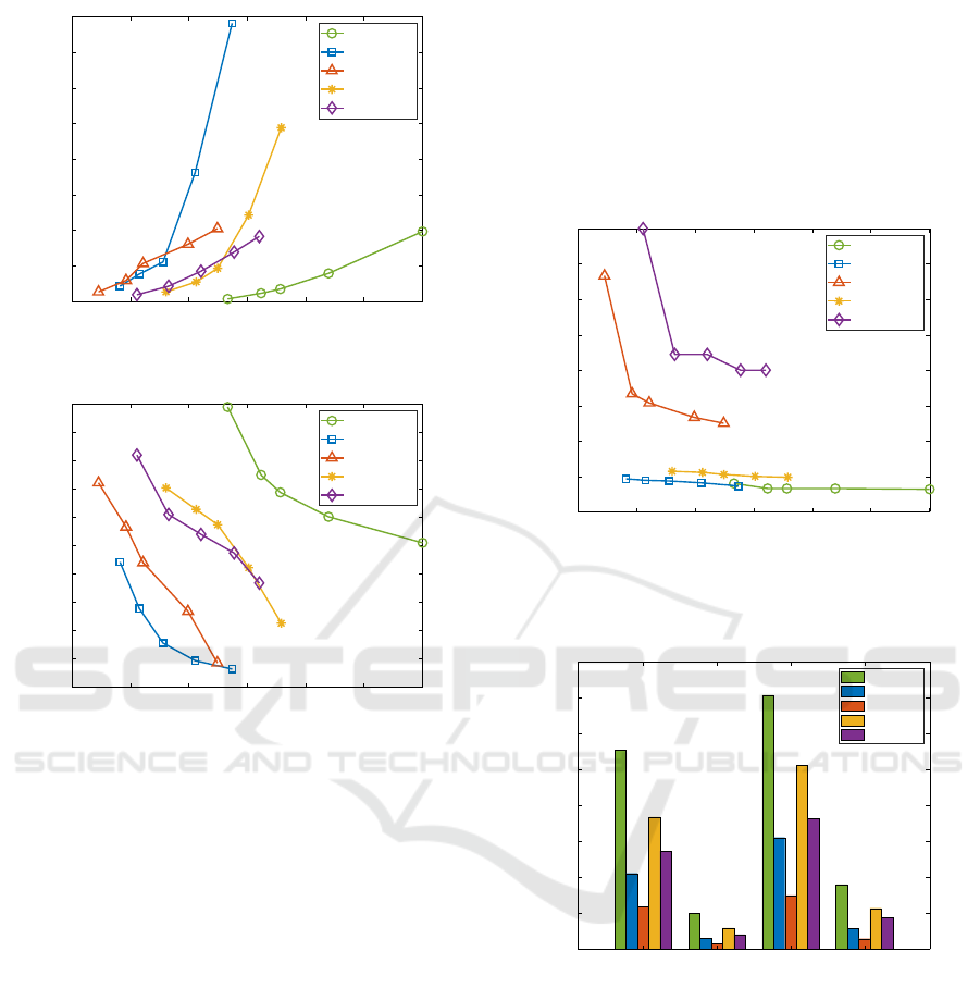
dicates perfect anti-correlation. Figure 6 shows the
average normalized error and SSIM values of the de-
compressed frames for each method.
From Figure 6(a), it is evident that our method
achieves the lowest normalized error while maintain-
ing the highest compression ratio. The same trend
holds true for the SSIM metric, as shown in Figure
6(b). Our method attains an SSIM value of 0.99,
indicating that the structural integrity of the original
frame is preserved nearly unchanged in the decom-
pressed frame. In Figure 6, it is interesting to note that
Real-Time Network-Aware Roadside LiDAR Data Compression
143

0 25 50 75 100 125 150
Compression Factor
0
0.05
0.1
0.15
0.2
0.25
0.3
0.35
0.4
Normalized Error
Ours
Draco
G-PCC
BF-Draco
BF-GPCC
(a) Normalized error
0 25 50 75 100 125 150
Compression Factor
0.5
0.55
0.6
0.65
0.7
0.75
0.8
0.85
0.9
0.95
1
SSIM
Ours
Draco
G-PCC
BF-Draco
BF-GPCC
(b) SSIM
Figure 6: Reconstruction error of each method for different
compression factors.
BF-Draco and BF-GPCC exhibit lower reconstruction
errors than Draco and G-PCC, respectively. Since
backgrounds are filtered in BF-Draco and G-PCC, the
frames contain less noise, resulting in reduced recon-
struction errors.
4.6 Communication Efficiency
The primary objectives of our proposed compression
system include enabling real-time streaming and fa-
cilitating massive device connectivity across multiple
traffic intersections through a shared private 5G net-
work. To this extent, we examine two key aspects: the
average compression time per frame for each method
and the number of LiDARs that can be streamed using
each method.
4.6.1 Compression Speed
Typically, a LiDAR sensor generates a frame every
100 milliseconds (ms). Therefore, the compression
time must be less than 100 ms to enable real-time
streaming without any frame drops. Figure 7 shows
the compression time of each method. Our method
takes only 20 ms to compress a frame, which is way
below the latency requirement of streaming LiDAR
data in real-time. Draco has similar compression
speed to ours, however, it fails to match our compres-
sion rate.
0 25 50 75 100 125 150
Compression Factor
0
25
50
75
100
125
150
175
200
Compression Time (ms)
Ours
Draco
G-PCC
BF-Draco
BF-GPCC
Figure 7: Compression speed comparison of each method
for different compression factors.
Ouster(16) Ouster(64) Livox Neuvition
Type of LiDARs
0
100
200
300
400
500
600
700
800
Number of LiDARs
Ours
Draco
G-PCC
BF-Draco
BF-GPCC
Figure 8: Number of supported LiDARs using each method
considering 250 Mbps private 5G bandwidth.
4.6.2 Number of Streamed LiDARs
Considering the bandwidth of a shared private 5G net-
work is 250 Mbps, Figure 8 illustrates how many Li-
DAR devices from different vendors can be streamed
using each method. In Figure 8, we can observe that
our method enables the transmission of data from
hundreds of LiDAR sensors, regardless of vendor
types, through a shared private 5G network. This rep-
resents at least 2.5 times more capacity than the base-
lines.
VEHITS 2025 - 11th International Conference on Vehicle Technology and Intelligent Transport Systems
144

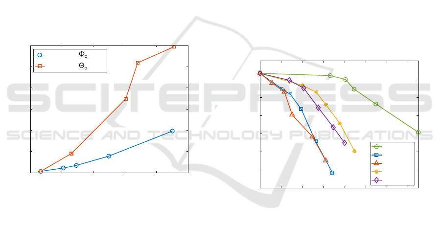
4.7 Parameter Sensitivity for Network
Awareness
In this section, we will discuss how we can adjust
the compression rate according to the available net-
work bandwidth by compromising a tolerable level
of compression quality. Our algorithm relies on two
parameters, φ
c
and θ
c
, which control the dimensions
of the range map. Increasing these parameters re-
duces the size of the range map, resulting in a higher
compression rate but lower compression quality. To
achieve the best compression quality, we set φ
c
and
θ
c
to φ
l
and θ
l
, respectively, which correspond to
LiDAR’s vertical and horizontal resolutions. Con-
sequently, when we have access to the full network
bandwidth, these values remain unchanged. However,
during network congestion, we have the flexibility to
increase either φ
c
or θ
c
to boost the compression rate.
Figure 9 shows the impact of increasing one of these
parameters while keeping the other constant on the re-
construction errors, specifically, the normalized error.
60 80 100 120 140 160
Compression Factor
0
0.05
0.1
0.15
0.2
0.25
0.3
Normalized Error
Increasing
Increasing
Figure 9: Parameter sensitivity test to identify which pa-
rameter is best to control compression rate with varying net-
work bandwidth.
In Figure 9, the blue curve depicts the compres-
sion factor and the corresponding normalized error
when θ
c
is held constant while φ
c
is set to φ
l
, 1.25∗φ
l
,
1.5 ∗φ
l
, 1.75 ∗φ
l
, and 2 ∗φ
l
. For the orange curve, φ
c
remains fixed while θ
c
is set to θ
l
, 1.25 ∗θ
l
, 1.5 ∗θ
l
,
1.75 ∗θ
l
, and 2 ∗θ
l
. It is evident from Figure 9 that
increasing φ
c
leads to a gradual increase in the nor-
malized error as the compression factor rises. How-
ever, increasing θ
c
results in a rapid escalation of the
normalized error. Consequently, we propose adapting
φ
c
according to the available network bandwidth to
control the compression factor effectively.
4.8 Application Accuracy
Superior compression capability is not useful if down-
stream applications are adversely affected by the use
of decompressed data, signifying the loss of valu-
able information during the compression process. To
demonstrate the effectiveness of the decompressed
data, we select two applications: i) vehicle counting,
and ii) object tracking, and conduct an analysis of the
accuracy of these tasks.
4.8.1 Vehicle Counting
Vehicle counting is a straightforward yet valuable ap-
plication, as it assists in assessing traffic congestion.
We employ the vehicle counting algorithm imple-
mented by (Mollah et al., 2022), which utilizes the
DBSCAN clustering algorithm on the background-
filtered data. To establish the ground truth dataset, we
randomly select 100 point cloud frames and manually
count the number of vehicles in each frame. Figure
10 illustrates the vehicle counting accuracy of each
method at different compression factors.
0 20 40 60 80 100 120 140
Compression Factor
30
40
50
60
70
80
90
100
Accuracy (%)
Ours
Draco
G-PCC
BF-Draco
BF-GPCC
Figure 10: Vehicle counting accuracy using decompressed
data produced by each methods.
In Figure 10, we observe that the application
achieves an accuracy of 93% using raw data. In con-
trast, when using the decompressed data generated by
our method, the application achieves a 92% accuracy
at a 66x compression factor, indicating minimal loss
of valuable information. In the case of G-PCC, the ap-
plication accuracy is 88%, but the compression factor
is only 11x. For Draco-decompressed data, the high-
est accuracy achieved is 85% with a compression fac-
tor of 20x. Across all methods, the accuracy of the ap-
plication decreases as the compression rate increases.
However, our method exhibits the lowest accuracy re-
duction rate compared to other baseline methods.
Real-Time Network-Aware Roadside LiDAR Data Compression
145

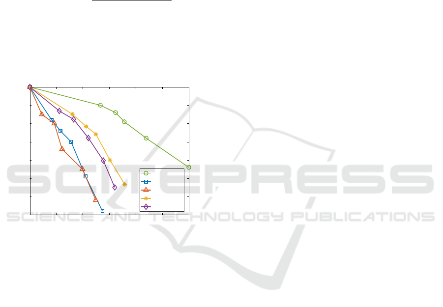
4.8.2 Object Tracking
For the object tracking application, we employ the
PointNet deep learning model (Charles et al., 2017) to
detect and track objects. Due to the absence of ground
truth labels, we utilize the tracking results on the raw
data as the ground truth. To assess the performance
of each method, we use the Multiple Object Tracking
Accuracy (MOTA) as the metric, which is computed
as follows:
MOTA = 1 −
∑
t
FN
t
+ FP
t
+ ME
t
∑
t
GT
t
, (5)
where, FN = false negatives, FP = false positives,
ME = missmatch errors, and GT = ground truth ob-
ject count. MOTA ranges from -inf to 1, where values
close to 1 suggest good accuracy, while values close
to 0 or less than 0 indicate poor accuracy.
0 25 50 75 100 125 150
Compression Factor
0.3
0.4
0.5
0.6
0.7
0.8
0.9
1
MOTA
Ours
Draco
G-PCC
BF-Draco
BF-GPCC
Figure 11: Object tracking accuracy using decompressed
data generated by each method.
Figure 11 illustrates the object tracking perfor-
mance of each method for various compression fac-
tors. Since the results of the raw data are consid-
ered as ground truth, the MOTA value is 1.0 for no
compression. The decompressed data produced by
our method achieve a MOTA value of 0.90, which
is slightly lower than the tracking results of the raw
data. However, it is still satisfactory, as the baseline
methods obtain a MOTA value of up to 0.85 with sig-
nificantly lower compression rates than ours.
5 CONCLUSION
In this paper, we propose a real-time compression
method for roadside LiDAR data. Our method ex-
ploits the unique characteristic of roadside LiDAR
data that the background points are repeated across
all frames. We first detect and send the background
points to the edge servers only once. Then, we fil-
ter the background points for each frame and only
compress the filtered frames. This achieves sub-
stantial temporal compression and significant spatial
compression. Our method is sensor-agnostic, fast,
memory-efficient, and adaptive to varying network
conditions. It achieves 2.5x higher compression rates
and 40% better application-level accuracy than the
state-of-the-art methods. Experimental results show
that our method is effective in compressing roadside
LiDAR data while maintaining high accuracy. It can
be used to stream raw data from sensors across mul-
tiple intersections in real time, enabling a wide range
of ITS applications.
REFERENCES
Charles, R., Su, H., Kaichun, M., and Guibas, L. J. (2017).
Pointnet: Deep learning on point sets for 3d classifi-
cation and segmentation. In 2017 IEEE Conference
on Computer Vision and Pattern Recognition (CVPR),
pages 77–85, Los Alamitos, CA, USA. IEEE Com-
puter Society.
Feng, Y., Liu, S., and Zhu, Y. (2020). Real-time
spatio-temporal lidar point cloud compression. 2020
IEEE/RSJ International Conference on Intelligent
Robots and Systems (IROS), pages 10766–10773.
Fischler, M. A. and Bolles, R. C. (1981). Random sample
consensus: A paradigm for model fitting with appli-
cations to image analysis and automated cartography.
24(6).
Golla, T. and Klein, R. (2015). Real-time point cloud com-
pression. In 2015 IEEE/RSJ International Confer-
ence on Intelligent Robots and Systems (IROS), page
5087–5092. IEEE Press.
Google (2018). Draco: 3d data compression. https://google.
github.io/draco/.
Guan, F., Xu, H., and Tian, Y. (2023). Evaluation of road-
side lidar-based and vision-based multi-model all-
traffic trajectory data. Sensors, 23(12).
Krivoku
´
ca, M., Chou, P. A., and Koroteev, M. (2020). A
volumetric approach to point cloud compression
˜
part
ii: Geometry compression. Trans. Img. Proc.,
29:2217–2229.
Lasserre, S., Flynn, D., and Qu, S. (2019). Using neighbour-
ing nodes for the compression of octrees representing
the geometry of point clouds. New York, NY, USA.
Association for Computing Machinery.
Li, S. and Yoon, H.-S. (2023). Vehicle localization in 3d
world coordinates using single camera at traffic inter-
section. Sensors, 23(7).
Lin, C., Zhang, H., Gong, B., Wu, D., and Wang, Y.-J.
(2023). Density variation-based background filtering
algorithm for low-channel roadside lidar data. Optics
& Laser Technology, 158:108852.
Lv, B., Xu, H., Wu, J., Tian, Y., and Yuan, C. (2019).
VEHITS 2025 - 11th International Conference on Vehicle Technology and Intelligent Transport Systems
146

Raster-based background filtering for roadside lidar
data. IEEE Access, 7:76779–76788.
Mollah, M. P., Debnath, B., Sankaradas, M., Chakradhar,
S., and Mueen, A. (2022). Efficient compression
method for roadside lidar data. In The 31st ACM Inter-
national Conference on Information and Knowledge
Management, page 3371–3380.
Nievergelt, Y. (1994). Total least squares: State-of-the-
art regression in numerical analysis. SIAM Review,
36(2):258–264.
Piadyk, Y., Rulff, J., Brewer, E., Hosseini, M., Ozbay, K.,
Sankaradas, M., Chakradhar, S., and Silva, C. (2023).
Streetaware: A high-resolution synchronized multi-
modal urban scene dataset. Sensors, 23(7).
Rossignac, J., Safonova, A., and Szymczak, A. (2001). 3d
compression made simple: Edgebreaker on a corner-
table.
Rusu, R. B. and Cousins, S. (2011). 3D is here: Point Cloud
Library (PCL). In IEEE International Conference on
Robotics and Automation (ICRA), Shanghai, China.
Sun, X., Ma, H., Sun, Y., and Liu, M. (2019). A novel point
cloud compression algorithm based on clustering.
IEEE Robotics and Automation Letters, 4(2):2132–
2139.
Thanou, D., Chou, P. A., and Frossard, P. (2016). Graph-
based compression of dynamic 3d point cloud se-
quences. IEEE Transactions on Image Processing,
25(4):1765–1778.
Tu, C., Takeuchi, E., Carballo, A., and Takeda, K. (2019).
Point cloud compression for 3d lidar sensor using re-
current neural network with residual blocks. In 2019
International Conference on Robotics and Automation
(ICRA), pages 3274–3280.
Wang, Z., Bovik, A., Sheikh, H., and Simoncelli, E. (2004).
Image quality assessment: from error visibility to
structural similarity. IEEE Transactions on Image
Processing, 13(4):600–612.
Wu, J., Xu, H., Sun, Y., Zheng, J., and Yue, R. (2018). Au-
tomatic background filtering method for roadside lidar
data. Transportation Research Record, 2672(45):106–
114.
Zhao, J., Xu, H., Chen, Z., and Liu, H. (2023). A decoding-
based method for fast background filtering of road-
side lidar data. Advanced Engineering Informatics,
57:102043.
Zhao, J., Xu, H., Xia, X., and Liu, H. (2019). Azimuth-
height background filtering method for roadside lidar
data. In 2019 IEEE Intelligent Transportation Systems
Conference (ITSC), pages 2421–2426.
Real-Time Network-Aware Roadside LiDAR Data Compression
147