Upside-Down Reinforcement Learning for More Interpretable Optimal

Control

Juan Cardenas-Cartagena

1,2

, Massimiliano Falzari

1,3

, Marco Zullich

and Matthia Sabatelli

Bernoulli Institute, University of Groningen, Groningen, The Netherlands

Wisenet Center, University of Agder, Grimstad, Norway

Data & Analytics R&I, ENGINEERING, Rome, Italy

Keywords:

Upside-Down Reinforcement Learning, Neural Networks, Random Forests, Interpretability, Explainable AI.

Abstract:

Model-Free Reinforcement Learning (RL) algorithms either learn how to map states to expected rewards or

search for policies that can maximize a certain performance function. Model-Based algorithms instead, aim

to learn an approximation of the underlying model of the RL environment and then use it in combination with

planning algorithms. Upside-Down Reinforcement Learning (UDRL) is a novel learning paradigm that aims

to learn how to predict actions from states and desired commands. This task is formulated as a Supervised

Learning problem and has successfully been tackled by Neural Networks (NNs). In this paper, we investigate

whether function approximation algorithms other than NNs can also be used within a UDRL framework.

Our experiments, performed over several popular optimal control benchmarks, show that tree-based methods

like Random Forests and Extremely Randomized Trees can perform just as well as NNs with the signiﬁcant

beneﬁt of resulting in policies that are inherently more interpretable than NNs, therefore paving the way for

more transparent, safe, and robust RL.

1 INTRODUCTION

The dramatic growth in adoption of Neural Net-

works (NNs) within the last 15 years has sparked

the necessity for increased transparency, especially in

high-stake applications (HLEG, 2019; Agarwal and

Mishra, 2021): NNs are indeed considered to be black

boxes whose rules for outputting predictions are non-

interpretable to humans. The quest for transparency

considers two different routes: interpretability and ex-

plainability (Broniatowski et al., 2021). Interpretabil-

ity is deﬁned as an inherent property of a model, and

it is well known that NNs lie very low on the inter-

pretability spectrum, whereas other methods, like de-

cision trees and linear models, are generally consid-

ered highly interpretable (James et al., 2013). Ex-

plainability, on the other hand, pertains to a series of

techniques that can be applied in a post-hoc fashion,

typically after a model has been trained, in order to

gain human-understandable insights on its inner dy-

namics. The downside of these techniques is that they

often approximate complex model dynamics; and is-

sues such as unfaithfulness (Nauta et al., 2023; Mir

Nicolau et al., 2025) arise. So, while NNs can of-

ten offer accurate solutions and state of the art per-

formance, interpretability has to be achieved through

inherently transparent models. When it comes to

high-stake applications Rudin (2019) argues that in-

terpretability is generically a more important prop-

erty than explainability. Among such high-stake ap-

plications, we can ﬁnd the management of decision

making systems that are applied to a large variety of

domains, ranging from healthcare to energy manage-

ment and even ﬁnancial risk assessment. Interest-

ingly, the recent marriage between Deep and Rein-

forcement Learning (DRL), has led to the develop-

ment of several systems that have successfully been

applied to these high-stake decision making prob-

lems. Examples of such applications go from the

aforementioned medical domain (Yu et al., 2021) to

particle physics (Degrave et al., 2022), infrastruc-

ture management planning (Leroy et al., 2024) and,

of course, autonomous driving (Sallab et al., 2017).

Unfortunately, despite working really well in prac-

tice, DRL algorithms carry over some of the limita-

tions that characterize NNs, therefore resulting in au-

tonomous agents whose optimal decision making ca-

pabilities are not interpretable nor fully explainable.

While Glanois et al. (2024) survey the efforts made

by researchers to use interpretable models, such as

rules-based methods or formulas, to explain transi-

tions or policies, it is worth mentioning that within the

extremely rapidly growing research landscape of Re-

inforcement Learning (RL), scientiﬁc works that are

Cardenas-Cartagena, J., Falzari, M., Zullich, M. and Sabatelli, M.

Upside-Down Reinforcement Learning for More Interpretable Optimal Control.

DOI: 10.5220/0013299400003890

Paper published under CC license (CC BY-NC-ND 4.0)

In Proceedings of the 17th International Conference on Agents and Artiﬁcial Intelligence (ICAART 2025) - Volume 1, pages 859-869

ISBN: 978-989-758-737-5; ISSN: 2184-433X

859

focused on this area are at the present moment rather

limited.

Contributions. In this paper, we aim to make one

step forward toward the development of more trans-

parent optimal decision making agents. To achieve

this, we rely on a newly introduced learning paradigm

that aims to solve typical RL problems from a

pure Supervised Learning perspective called Upside

Down Reinforcement Learning (UDRL) (Schmidhu-

ber, 2019). While originally designed for being cou-

pled with NNs, we show that an UDRL approach can

also be successfully integrated with inherently more

interpretable machine learning models, like forests of

randomized trees. Despite not being as interpretable

as simple decision trees (James et al., 2013), this fam-

ily of techniques still offers an intrinsic tool for global

feature importance, such as mean decrease in impu-

rity, thus offering an edge over NNs in terms of inter-

pretability (Ibrahim et al., 2019) and design of trans-

parent autonomous agents.

2 UPSIDE-DOWN

REINFORCEMENT LEARNING

2.1 The UDRL Framework

The concept of Upside-Down Reinforcement Learn-

ing (UDRL) was ﬁrst introduced by Schmidhuber

(2019), and its idea is remarkably straightforward:

tackling Reinforcement Learning problems via Su-

pervised Learning (SL) techniques. To understand

how this can be achieved, let us introduce the typical

Markovian mathematical framework on which pop-

ular RL algorithms are based. We deﬁne a Markov

Decision Process (MDP) (Puterman, 2014) as a tuple

M = ⟨S , A, P , R ⟩ where S corresponds to the state

space of the environment, A is the action space mod-

eling all the possible actions available to the agent,

P : S × A × S → [0, 1] is the transition function and

R : S × A × S → R is the reward function. When

interacting with the environment, at each time-step t,

the RL agent performs action a

in state s

, and tran-

sitions to state s

t+1

alongside observing reward signal

. The goal is then to learn a policy π : S → ∆(A)

which maximizes the expected discounted sum of re-

wards E

[

∑

∞

k=0

t+k

], with γ ∈ [0, 1). It is well

known that when it comes to RL, differently from the

Dynamic Programming setting, the transition func-

tion P and the reward function R are unknown to the

agent. To overcome this lack of information, the agent

can either learn to predict expected rewards, assuming

the model-free RL set-up, or learn to predict s

t+1

and

, assuming a model-based RL setting.

In UDRL the agent doesn’t do either, and its main

goal is learning to predict actions instead. Given a

typical RL transition τ = ⟨s

, a

, r

, s

t+1

⟩, an UDRL

agent uses the information contained within τ to learn

to map a certain state s

, and reward r

to action

. Formally, this corresponds to learning a function

f (s

, r

) = a

, a task that can be seen as a classic SL

problem where the goal is that of building a function

f : X → Y , where X and Y are the input and output

spaces deﬁning the SL problem one wants to solve.

While intuitive and easy to understand, the function

deﬁned above does not account for long-horizon re-

wards, which are crucial for most optimal control

problems. Therefore, it needs to be slightly modiﬁed.

This can be achieved by introducing two additional

variables that come with the name of commands: d

and d

. They correspond to the desired reward d

the

agent wants to achieve within a certain time horizon

when being in state s

. Based on this, we can deﬁne

the ultimate goal of a UDRL agent as that of learn-

ing f (s

, d

) = a

. This function f comes with the

name of behavior function and, ideally, if learned on

a large number of transitions τ, it can be queried in

such a way that it can return the action that achieves

a certain reward in a certain state in a certain number

of time-steps. To better understand the role of this

behavior function, let us consider the simple MDP

represented in Figure 1, where states are denoted as

nodes and edges are represented by the actions a the

agent can take, alongside the rewards r

the agent ob-

serves.

= 2

= 1

= −1

Figure 1: A simple MDP whose behavior function f is sum-

marized in Table 1.

A fully trained behavior function that correctly

models the dynamics of this MDP is summarized in

Table 1.

Related Work. The ﬁrst successful application of

the UDRL paradigm can be found in the work of Sri-

vastava et al. (2019), who showed that a UDRL agent

controlled by a neural network could outperform pop-

IAI 2025 - Special Session on Interpretable Artiﬁcial Intelligence Through Glass-Box Models

860

Table 1: A tabular representation of the behavior function f

that correctly models the dynamics represented in the MDP

visualized in Figure 1. For example, let us consider that

the agent is in state s

and that its goal is that of obtaining

a desired reward of d

= 2 in one time-step d

, then when

queried this function should return a

. Note how the infor-

mation contained within s

, concatenated to d

and d

, con-

stitutes a training sample that can be used in an SL setting

for predicting a

State d

Action a

2 1 a

1 1 a

1 2 a

-1 1 a

ular model-free RL algorithms such as DQN and PPO

on both discrete and continuous action space environ-

ments. The same paper also highlights the potential of

UDRL when it comes to sparse-reward environments.

UDRL has been subsequently applied by Ashley et al.

(2022) and Arulkumaran et al. (2022) with the latter

work showcasing how this learning paradigm can be

successfully extended to a setting of ofﬂine RL, im-

itation learning, and even meta-RL. While the term

UDRL has only been introduced very recently, it is

worth mentioning that some of its core ideas can

be associated with the ﬁelds of goal-conditioned or

return-conditioned RL (Liu et al., 2022; Furuta et al.,

2021). In this learning set-up agents need to learn ac-

tions constrained to particular goals, which may come

in the form of speciﬁc rewards in given states, usu-

ally from hindsight information. Besides these works,

UDRL has, to the best of our knowledge, seldom

been applied in other studies if not for comparing it

with other similar techniques, such as the Decision

Transformer (Chen et al., 2021). This highlights how

UDRL is still an underexplored technique that is still

far from expressing its potential.

3 METHODS

In all of the applications above of UDRL, f comes

in the form of a neural network, a choice motivated

by the recent successes that this family of machine

learning techniques has demonstrated when it comes

to RL problems modeled by high-dimensional state

and action spaces. However, the UDRL formalism in-

troduced by Schmidhuber (2019) allows for using any

machine learning algorithm suitable for solving SL

tasks. Yet, to the best of our knowledge, no such study

exists. In what follows, we start by exploring whether

ﬁve different SL algorithms can be effectively cou-

pled with the UDRL framework and therefore provide

a valuable alternative to NNs. A brief description of

these algorithms, alongside an explanation about why

they were chosen, is presented hereafter.

3.1 Algorithms

Tree-Based Algorithms. The ﬁrst two studied al-

gorithms can be categorized under the tree-based

Reinforcement Learning umbrella and are Random

Forests (RFs) (Breiman, 2001) and Extremely Ran-

domized Trees (ETs) (Geurts et al., 2006). Differ-

ent from neural networks, both methods are nonpara-

metric and build a model in the form of the average

prediction of an ensemble of regression trees. Be-

fore the advent of neural networks, they both provided

a valuable choice of function approximation within

the realm of approximate Reinforcement Learning

(Busoniu et al., 2017) and have successfully been

used for solving several optimal control problems.

For example, RFs were successfully coupled with

the popular Q-Learning algorithm by Min and Elliott

(2022), which showed on-par performance to that of

Deep-Q Networks on two of the three studied bench-

marks. They were also successfully used in a multi-

objective setting by Song and Wang (2024), who

optimized multiple objectives in a multistage medi-

cal multi-treatment setting. Regarding ETs, the ar-

guably most successful application is that presented

by Ernst et al. (2005), where ETs were used to con-

struct the popular Fitted Q Iteration algorithm for the

batch RL setting. ETs have since then been suc-

cessfully used for solving several RL tasks, ranging

from the design of clinical trials (Ernst et al., 2006b;

Zhao et al., 2009) to the management of intensive care

units (Prasad et al., 2017) and even autonomous driv-

ing (Mirchevska et al., 2017). Among the beneﬁts

of this family of techniques Wehenkel et al. (2006)

highlight their universal approximation consistency,

alongside their interpretability, two properties which,

in the UDRL context, could allow learning an inter-

pretable and transparent behavior function f .

Boosting Algorithms. The third and fourth stud-

ied behavior functions are ensemble methods that fall

within the boosting family of algorithms. Differ-

ently from the aforementioned tree-based algorithms,

which construct the trees independently and in par-

allel, boosting techniques build the trees sequentially,

with the main goal of having each new tree learn from

the errors of the previous one. While several boost-

ing algorithms exist, in this paper we consider the

two arguably most popular ones: AdaBoost (Freund

et al., 1996) and XGBoost (Friedman, 2001). Both of

these algorithms have successfully been used in RL

Upside-Down Reinforcement Learning for More Interpretable Optimal Control

861

(Brukhim et al., 2022), although their RL applications

are scarcer compared to RFs and ETs. Yet, we be-

lieve that within the UDRL setting, they both could

be used for effectively learning the behavior function

f . As was described in Table 1, a typical UDRL be-

havior function is trained on data that comes in tabular

form, a data type on which boosting algorithms typi-

cally perform very well and can even outperform NNs

(Shwartz-Ziv and Armon, 2022).

K-Nearest Neighbour. The ﬁnal considered algo-

rithm is K-Nearest Neighbour (KNN) (Cover and

Hart, 1967), a popular clustering method rooted in

instance-based learning. While its applications when

it comes to RL are rather limited, made some excep-

tions for its integration within some model-free algo-

rithms (Mart

ın H et al., 2009; Shah and Xie, 2018),

this algorithm was chosen as it provides a straightfor-

ward non-parametric baseline that can be effectively

used for assessing the performance of the previously

introduced tree-based and boosting methods.

3.2 Environments

We evaluate the performance of the abovementioned

algorithms on three popular optimal control bench-

marks of increasing difﬁculty. The benchmarks are

CartPole (Barto et al., 1983), Acrobot (Sutton,

1995) and Lunar Lander and are all provided by the

OpenAI-Gym package. Each environment is summa-

rized in Table 2, where we describe its key compo-

nents, by speciﬁcally focusing on the state space S

representation, as this information will play an im-

portant role in Section 5 of the paper.

3.3 Experimental Setup

We train each behavior function on the aforemen-

tioned optimal control tasks ﬁve times with ﬁve differ-

ent random seeds by following the algorithmic guide-

lines described by Srivastava et al. (2019), the full

pseudo-code of our UDRL implementation can be

found in the Appendix 6. Each algorithm is allocated

a budget of 500 training episodes, as this is a num-

ber of episodes that are known to be sufﬁcient for re-

sulting in successful learning for most popular DRL

algorithms. When it comes to the NN, the behavior

function comes in the form of a multi-layer percep-

tron with three hidden layers, activated by ReLU ac-

tivation functions. The size of each hidden layer is 64

nodes and the popular Adam algorithm with a learn-

ing rate of 0.001 is used for optimization. The net-

work is implemented in the PyTorch deep-learning

framework (Paszke et al., 2017). All other behavior

functions are implemented with the Scikit-Learn

package (Pedregosa et al., 2011) and we adopt the de-

fault hyperparameters that are provided by the library.

Exploration of all agents is governed via the popular

ε-greedy strategy with the value of ε set constant to

0.2 throughout training. Lastly, as is common prac-

tice, all behavior functions are trained on UDRL tran-

sitions that are stored in an Experience-Replay mem-

ory buffer which has a capacity of 700.

4 RESULTS

We now provide an analysis of the performance of the

six different tested behavior functions f . Our analy-

sis is twofold: ﬁrst, we focus on the performance ob-

tained at training time, while later we focus on the

performance obtained at inference time.

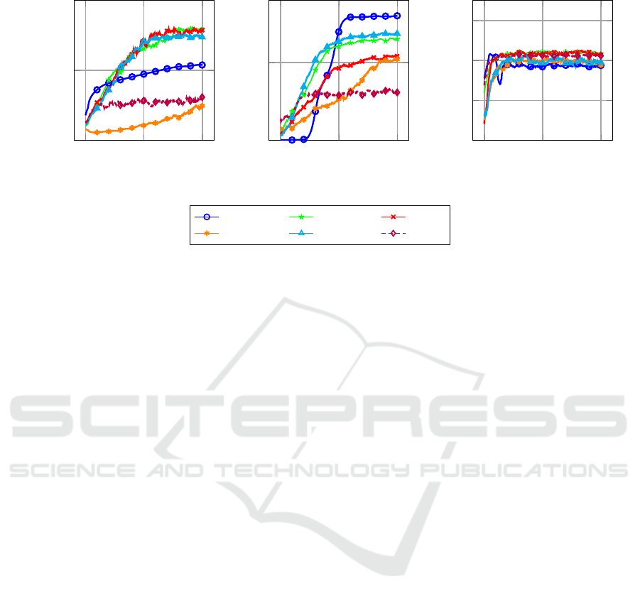
Training. Our training curves are reported in Fig-

ure 2 where for each algorithm we show the average

reward obtained per training episode over ﬁve differ-

ent training runs. We can start by observing that on

the CartPole task the best-performing behavior func-

tions appear to be RFs, ETs, and XGBoost, as they all

obtain training rewards of ≈ 150. The performance of

these ensemble methods is therefore better than that

obtained by the NN, which, despite showing some

faster initial training, obtains a ﬁnal reward of ≈ 100.

The KNN and AdaBoost behavior functions on the

other hand show less promising results as their perfor-

mance only marginally improves over training. When

it comes to the Acrobot task we can observe that this

time the best performing algorithm is the NN, as it

converges to a training reward of ≈ −150. Among

the tree-based methods, the RF behavior function is

the one performing best, obtaining training rewards

of ≈ −200. A similar performance is also obtained

by the XGBoost algorithm. ETs and AdaBoost even-

tually perform very similarly although the ET al algo-

rithm converges signiﬁcantly faster. Similar to what

was observed on the CartPole task, the worst per-

forming algorithm is again the KNN behavior func-

tion. On the Lunar Lander environment we can ob-

serve that all tested behavior functions are able to im-

prove their decision making across episodes. There-

fore, suggesting that there is no algorithm that signif-

icantly outperforms all of the others.

Inference. While the results presented above are

promising and possibly suggest that in the UDRL

context the behavior function f does not have to nec-

essarily come in the form of a neural network, it is

essential to investigate how general and robust this

IAI 2025 - Special Session on Interpretable Artiﬁcial Intelligence Through Glass-Box Models

862

Table 2: An overall description of the CartPole, Acrobot, and Lunar Lander environments used in our experiments. For

each environment, we report information regarding its state S and A action spaces, together with the rewards that the agent

receives while interacting.

Component CartPole Acrobot Lunar Lander

States S Continuous 4D vector:

- x: Cart Position

- ˙x: Cart Velocity

- θ: Pole Angle

θ: Pole Angular Velocity

Continuous 6D vector:

- sinθ

: Sine of the ﬁrst link

- cosθ

: Cosine of the ﬁrst link

- sinθ

: Sine of the second link

- cosθ

: Cosine of the second link

: Angular velocity of ﬁrst link

: Angular velocity of second link

Continuous 8D vector:

- x: X position

- y: Y position

- ˙x: X linear velocity

- ˙y: Y linear velocity

- θ: Angle

θ: Angular velocity

- Left and right leg contact points

Actions A Discrete:

0: Push left

1: Push right

Discrete:

0: Torque left

1: No torque

2: Torque right

Discrete:

0: Do nothing

1: Fire left engine

2: Fire main engine

3: Fire right engine

Rewards r

+1 for every step taken -1 for every step until the goal is reached +100 for successful landing

-100 for crash landing

Reward for ﬁring engines and leg contact

behavior function is. Note that, as was described

in Section 3.3, the results presented in Figure 2 are

computed at training time, which means that the re-

ported performance is representative of the ε-greedy

exploration strategy that the algorithms follow whilst

training. As a result, the performance presented in

the above-mentioned training curves is only partially

representative of the ﬁnal performance of the differ-

ent algorithms. To quantitatively assess how well

the trained behavior functions have actually mastered

the three different optimal control environments, one

needs to query these functions. Recall, that based

on the formalism explained in Section 2, the ultimate

goal of UDRL is that of learning a behavior function

f , that once queried with a state coming from the en-

vironment s

can return action a

achieving desired

reward d

in time horizon d

. Therefore, to test the in-

ference capabilities of the different behavior functions

it is crucial to deﬁne d

and d

. For the CartPole task

this is straightforward as it is well known that given

the episodic nature of the problem, the maximum cu-

mulative reward an agent can obtain is that of 200. It

follows that all behavior functions are queried with d

and d

set to 200. When it comes to the Acrobot and

Lunar Lander environments, which differently from

CartPole are non-episodic tasks, setting d

and d

re-

quires some extra care. As one wants to avoid queer-

ing the behavior function with desired commands c

that are unrealistic and not supported by the environ-

ment, we decided to set d

and d

to the most com-

mon used values that were used throughout the last

100 episodes, as we believe they are fairly represen-

tative of the ﬁnal performance of the algorithms. For

each behavior function and environment, we report

the exact form of f (s

, d

) in Table 3.

Table 3: The form of the behavior function f that is used at

inference time by each algorithm on the three tested envi-

ronments.

Behaviour Function CartPole Acrobot Lunar Lander

Neural Network f (·,200, 200) f (·, −63, 64) f(·, 49, 101)

Random Forest f (·, 200,200) f (·, −79, 82) f (·, 57, 102)

Extra-Trees f (·, 200,200) f (·, −75, 77) f (·, 34, 118)

AdaBoost f (·, 200,200) f (·, −77, 81) f (·, 45, 118)

XGBoost f (·, 200,200) f(·, −114, 120) f (·, 136,389)

KNN f (·, 200,200) f(·, −129, 132) f (·, 62,112)

The results obtained at inference time are pre-

sented in Table 4 where we report the average cumu-

lative reward that is obtained by the behavior func-

tion presented in Table 3 which is queried 100 times.

The results of the best performing behavior function

are presented in a green cell, whereas the ones of the

second best performing one are reported in a yellow

cell. On the CartPole task we can observe that the

overall best performing behavior function is the one

coming in the form of a NN, followed by the one

modeled by the XGBoost algorithm, as both behavior

functions fully solve the presented task by obtaining

a ﬁnal cumulative reward of ≈ 200. The performance

of the tree-based algorithms is slightly lower, and a

bit more unstable as shown by the larger standard de-

viations, however, it can still be stated that both al-

gorithms have learned how to balance the cart suc-

cessfully. Good performance was also obtained by

the AdaBoost algorithm, albeit not on par with that

of the aforementioned tree-based algorithms. Finally,

the KNN behavior function remains the worst per-

forming algorithm as was already highlighted when

discussing the ﬁrst plot presented in Figure 2, where

Upside-Down Reinforcement Learning for More Interpretable Optimal Control

863

250 500

100

200

Episode

Reward

CartPole

250 500

−500

−250

−50

Episode

Acrobot

250 500

−250

−150

−50

Episode

Lunar Lander

NN RF ET

AdaBoost XGBoost

KNN

Figure 2: Comparison of the performance of the six different tested behavior functions (NN, RF, ET, KNN, AdaBoost, and

XGBoost) on the three OpenAI Gym environments: CartPole, Acrobot, and Lunar Lander. The results are shown in terms

of rewards per episode and are averaged over ﬁve different training runs.

the algorithm barely improved its decision making

over time. When it comes to the Acrobot task, we

can again see that the best performing behavior func-

tion is that modeled by a NN which obtains ﬁnal test-

ing rewards of ≈ −75. RFs, ETs, and XGBoost all

perform similarly, although their ﬁnal performance

is slightly worse compared to that of NNs given ﬁ-

nal testing rewards of ≈ −100. Again, we can note

that the results obtained by the AdaBoost algorithm

are not on-par with those obtained by the tree-based

methods and that the KNN algorithm is overall the

worse performing algorithm. On the arguably most

complicated Lunar Lander environment, we can see

that the best performing behavior function is the one

modeled via RFs, which obtains a ﬁnal performance

of ≈ −54. Similarly to what was observed on the

CartPole task the second best performing algorithm

is XGBoost, and perhaps surprisingly the third best

performing algorithm is AdaBoost. Arguably even

more surprising is the fact that on this task the KNN

behavior function managed to actually improve its

performance over time, and that the behavior function

modeled by the NN is the overall worst performing al-

gorithm.

5 INTERPRETABILITY GAINS

While RFs and ETs did not signiﬁcantly outperform

their NN counterparts in terms of ﬁnal performance,

it is worth noting that this family of techniques has

much more to offer regarding interpretability than

NNs as it allows us to get global explanations for the

behavior function, which in the case of NNs is not

straightforward. In this section, we aim to shed some

light on what makes the aforementioned tree-based

behavior functions able to solve the optimal control

tasks described in Section 3.2 almost optimally. To

this end, we rely on the work of Louppe et al. (2013):

for different states of the tested environments, we

compute feature importance scores that are estimated

as mean impurity decrease. We compute these scores

at inference time, based on the experimental protocol

that was discussed in the second paragraph of Section

4. We present a qualitative analysis that shows how

for different states of the environments, sampled at

different stages of the RL episode, the feature impor-

tance scores change and can highlight which features

of the state space S are the most relevant for the be-

havior function.

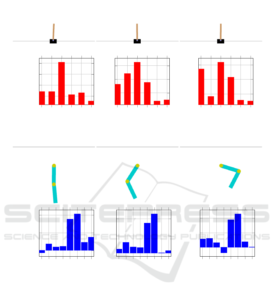
We start by discussing the scores obtained on the

CartPole task by an RF behavior function. These re-

sults are summarized in Figure 3. Overall we can ob-

serve that out of the four different features modeling

the state space, the highest importance score through-

out an episode is always associated with the pole an-

gular velocity θ feature, as demonstrated by all three

histogram plots of Figure 3. This feature appears to

play an even more signiﬁcant role when the pole on

top of the cart is in an out-of-balance position (see

ﬁrst plot of Figure 3). We can also observe that at

the very beginning of the episode (last plot of Fig-

ure 3), high-importance scores are associated with the

feature denoting the position of the cart x, although

the more the agent interacts with the environment, the

less important this feature becomes.

On the Acrobot environment, where we report

IAI 2025 - Special Session on Interpretable Artiﬁcial Intelligence Through Glass-Box Models

864

Table 4: The results of the six tested behavior functions obtained at inference time, namely when the behavior function f

gets queried with the desired reward d

and desired time horizon d

commands described in Table 3. The best performing

algorithm is reported in a green cell, whereas the second best performing algorithm is reported in a yellow cell.

Behavior Function CartPole Acrobot Lunar Lander

Neural Network 199.93 ± 0.255 −75.00 ± 15.36 −157.04 ± 71.26

Random Forest 188.25 ± 13.82 −100.05 ± 62.80 −54.74 ± 96.22

Extra-Trees 181.56 ± 31.63 −100.00 ± 93.72 −127.79 ± 49.19

AdaBoost 168.61 ± 31.02 −109.00 ± 63.70 −108.26 ± 80.71

XGBoost 199.27 ± 4.06 −100.00 ± 34.71 −76.96 ± 89.69

KNN 85.11 ± 50.30 −160.50 ± 36.66 −128.47 ± 47.49

feature importance scores for the ET behavior func-

tion, we can observe from the results presented in Fig-

ure 4 that the most important features are by far the

ones representing the two angularComparison with

State of the Art velocities of the two links (

and

). These two features are consistently associated to

the two highest importance scores, no matter at which

stage of the episode the agent is.

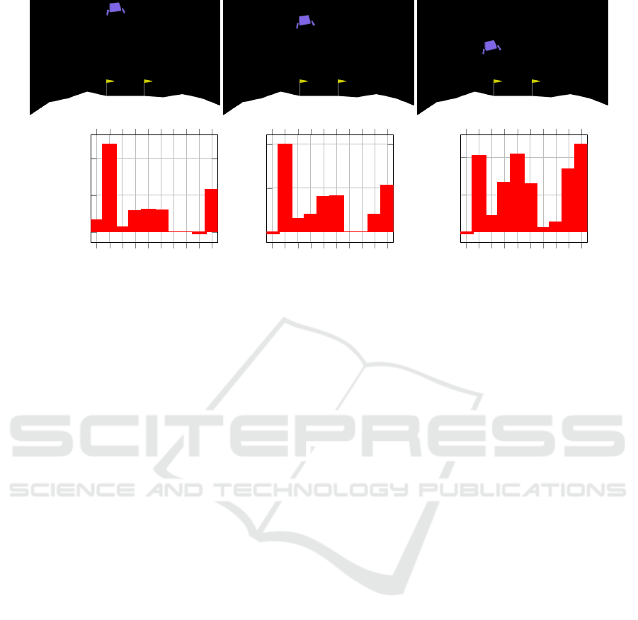
Finally, when it comes to the Lunar Lander envi-

ronment we have observed that by far the most impor-

tant feature of the environment is the one representing

the y position of the spaceship that is being controlled

by the agent. This can be seen in all three histograms

presented in Figure 5. Intuitively this is also a result

that seems to make sense, as the goal of the agent is

that of controlling the spaceship which is approach-

ing the moon’s surface from above. Interestingly, we

can also note that the features modeling the left and

right contact points of the spaceship, l

and l

, have

very low importance scores no matter how close the

spaceship is to the surface. Furthermore, it can also

be observed that when the spaceship is still far from

approaching the moon’s ground the importance scores

of the features denoting the linear velocity ( ˙y), as well

as the angle θ and angular velocity

θ of the spaceship

are fairly low. However, as highlighted by the third

plot of Figure 5 this changes once the spaceship is

about to land.

As the results presented in Figures 3, 4 and 5 are

only a snapshot of the full agent-environment inter-

action, we refer the reader to the webpage of this

project

where we release all trained behavior func-

tions whose inference performance can be tested in

the browser alongside the computation of the feature

importance scores for all states encountered by the

agent.

https://vimmoos-udrl.hf.space/

6 DISCUSSION & CONCLUSION

In this paper, we have explored the potential that Up-

side Down Reinforcement Learning has to offer when

it comes to the design of interpretable and transparent

autonomous agents. We have shown that the behav-

ior function f , which plays a crucial role in this novel

learning paradigm, does not have to strictly come in

the form of a neural network as originally described

by Schmidhuber (2019) and that tree-based ensem-

ble methods, together with boosting algorithms, can

perform just as well. We have also provided ini-

tial promising insights suggesting that behavior func-

tions coming in the form of Random Forests and Ex-

tremely Randomized Trees can have much more to

offer in terms of interpretability than their neural net-

work counterparts. Based on these results we fore-

see several promising avenues for future work. The

main, rather obvious, limitation of this paper is that it

considers overall simple optimal-control benchmarks,

which are far in terms of complexity from the RL en-

vironments that the DRL community adopts as test

beds. How well UDRL agents trained with RFs and

ETs would perform on high-dimensional and spa-

tially organized state spaces such as those modeled

by the popular Atari Arcade Learning Environment

is unknown. While it is well known that convolu-

tional neural networks have become the go-to design

choice when it comes to these types of problems, it is

worth mentioning that other valid alternatives could

be explored. For example, in the contexts of forests

of randomized trees, one could consider the work of

Mar

ee et al. (2005) and extend it from the value-based

RL setting, where it has shown promising results on

rather complex environments (Ernst et al., 2006a),

to the UDRL one. Next to scaling and generalizing

the results presented in this study to more complex

tasks, we believe another promising direction for fu-

ture work revolves around coupling the tree-based be-

havior functions with other explanation tools. Tech-

niques such as the recently introduced DPG (Arrighi

Upside-Down Reinforcement Learning for More Interpretable Optimal Control

865

˙x

Importance

˙x

Figure 3: Feature importance scores coming from a trained RF behavior function computed for three different states of the

CartPole environment. In the ﬁrst state, the agent decided to push the cart to the left, whereas in the second and third states,

the cart was pushed to the right.

sinθ

cosθ

sinθ

cosθ

Importance

sinθ

cosθ

sinθ

cosθ

sinθ

cosθ

sinθ

cosθ

Figure 4: Feature importance scores coming from a trained ET behavior function computed for three different states of the

Acrobot environment. In the ﬁrst state, the agent decided to not apply any torque, while in the second and third states left

and right torques were applied respectively.

et al., 2024) which helps with the identiﬁcation of

salient nodes in forests of randomized trees, or the

more popular Shapley values (Winter, 2002) along-

side their extensions (Muschalik et al., 2024) come

to mind. Lastly, it is worth highlighting the over-

all good performance obtained by the XGBoost al-

gorithm. While we have focused our interpretability

analysis on RFs and ETs, it is well-known that this al-

gorithm also has a lot to offer regarding feature impor-

tance scores. In the future, we aim to provide a thor-

ough comparison between different, inherently inter-

pretable behavior functions, to further identify which

state space components of an RL environment are the

most important ones to a UDRL agent.

REFERENCES

Agarwal, S. and Mishra, S. (2021). Responsible AI.

Springer.

Arrighi, L., Pennella, L., Marques Tavares, G., and Bar-

bon Junior, S. (2024). Decision predicate graphs:

Enhancing interpretability in tree ensembles. In

World Conference on Explainable Artiﬁcial Intelli-

gence, pages 311–332. Springer.

Arulkumaran, K., Ashley, D. R., Schmidhuber, J., and Sri-

vastava, R. K. (2022). All you need is supervised

learning: From imitation learning to meta-rl with up-

side down rl. arXiv preprint arXiv:2202.11960.

Ashley, D. R., Arulkumaran, K., Schmidhuber, J., and Sri-

vastava, R. K. (2022). Learning relative return poli-

IAI 2025 - Special Session on Interpretable Artiﬁcial Intelligence Through Glass-Box Models

866

˙x

˙y

Importance

˙x

˙y

˙x

˙y

Figure 5: Feature importance scores coming from a trained RF behavior function computed for three different states of the

Lunar Lander environment. In the ﬁrst and second states, the agent decided to ﬁre the main engine, while in the third state

it decided to ﬁre the right engine.

cies with upside-down reinforcement learning. arXiv

preprint arXiv:2202.12742.

Barto, A. G., Sutton, R. S., and Anderson, C. W. (1983).

Neuronlike adaptive elements that can solve difﬁcult

learning control problems. IEEE transactions on sys-

tems, man, and cybernetics, (5):834–846.

Breiman, L. (2001). Random forests. Machine learning,

45:5–32.

Broniatowski, D. A. et al. (2021). Psychological founda-

tions of explainability and interpretability in artiﬁcial

intelligence. NIST, Tech. Rep.

Brukhim, N., Hazan, E., and Singh, K. (2022). A boost-

ing approach to reinforcement learning. Advances

in Neural Information Processing Systems, 35:33806–

33817.

Busoniu, L., Babuska, R., De Schutter, B., and Ernst, D.

(2017). Reinforcement learning and dynamic pro-

gramming using function approximators. CRC press.

Chen, L., Lu, K., Rajeswaran, A., Lee, K., Grover, A.,

Laskin, M., Abbeel, P., Srinivas, A., and Mordatch, I.

(2021). Decision transformer: Reinforcement learn-

ing via sequence modeling. Advances in neural infor-

mation processing systems, 34:15084–15097.

Cover, T. and Hart, P. (1967). Nearest neighbor pattern clas-

siﬁcation. IEEE transactions on information theory,

13(1):21–27.

Degrave, J., Felici, F., Buchli, J., Neunert, M., Tracey, B.,

Carpanese, F., Ewalds, T., Hafner, R., Abdolmaleki,

A., de Las Casas, D., et al. (2022). Magnetic con-

trol of tokamak plasmas through deep reinforcement

learning. Nature, 602(7897):414–419.

Ernst, D., Geurts, P., and Wehenkel, L. (2005). Tree-based

batch mode reinforcement learning. Journal of Ma-

chine Learning Research, 6.

Ernst, D., Mar

ee, R., and Wehenkel, L. (2006a). Reinforce-

ment learning with raw image pixels as input state. In

Advances in Machine Vision, Image Processing, and

Pattern Analysis: International Workshop on Intelli-

gent Computing in Pattern Analysis/Synthesis, IWIC-

PAS 2006 Xi’an, China, August 26-27, 2006 Proceed-

ings, pages 446–454. Springer.

Ernst, D., Stan, G.-B., Goncalves, J., and Wehenkel, L.

(2006b). Clinical data based optimal sti strategies for

hiv: a reinforcement learning approach. In Proceed-

ings of the 45th IEEE Conference on Decision and

Control, pages 667–672. IEEE.

Freund, Y., Schapire, R. E., et al. (1996). Experiments with

a new boosting algorithm. In icml, volume 96, pages

148–156. Citeseer.

Friedman, J. H. (2001). Greedy function approximation: a

gradient boosting machine. Annals of statistics, pages

1189–1232.

Furuta, H., Matsuo, Y., and Gu, S. S. (2021). Generalized

decision transformer for ofﬂine hindsight information

matching. arXiv preprint arXiv:2111.10364.

Geurts, P., Ernst, D., and Wehenkel, L. (2006). Extremely

randomized trees. Machine learning, 63:3–42.

Glanois, C., Weng, P., Zimmer, M., Li, D., Yang, T., Hao,

J., and Liu, W. (2024). A survey on interpretable rein-

forcement learning. Machine Learning, pages 1–44.

HLEG, H.-L. E. G. o. A. (2019). Ethics guidelines for trust-

worthy ai.

Ibrahim, M., Louie, M., Modarres, C., and Paisley, J.

(2019). Global explanations of neural networks: Map-

ping the landscape of predictions. In Proceedings of

the 2019 AAAI/ACM Conference on AI, Ethics, and

Society, pages 279–287.

James, G., Witten, D., Hastie, T., Tibshirani, R., et al.

(2013). An introduction to statistical learning, vol-

ume 112. Springer.

Leroy, P., Morato, P. G., Pisane, J., Kolios, A., and Ernst, D.

(2024). Imp-marl: a suite of environments for large-

scale infrastructure management planning via marl.

Upside-Down Reinforcement Learning for More Interpretable Optimal Control

867

Advances in Neural Information Processing Systems,

36.

Liu, M., Zhu, M., and Zhang, W. (2022). Goal-

conditioned reinforcement learning: Problems and so-

lutions. arXiv preprint arXiv:2201.08299.

Louppe, G., Wehenkel, L., Sutera, A., and Geurts, P. (2013).

Understanding variable importances in forests of ran-

domized trees. Advances in neural information pro-

cessing systems, 26.

Mar

ee, R., Geurts, P., and Wehenkel, J. P. L. (2005). Ran-

dom subwindows for robust image classiﬁcation. In

2005 IEEE Computer Society Conference on Com-

puter Vision and Pattern Recognition (CVPR’05), vol-

ume 1, pages 34–40. IEEE.

Mart

ın H, J. A., de Lope, J., and Maravall, D. (2009). The

k nn-td reinforcement learning algorithm. In Methods

and Models in Artiﬁcial and Natural Computation. A

Homage to Professor Mira’s Scientiﬁc Legacy: Third

International Work-Conference on the Interplay Be-

tween Natural and Artiﬁcial Computation, IWINAC

2009, Santiago de Compostela, Spain, June 22-26,

2009, Proceedings, Part I 3, pages 305–314. Springer.

Min, J. and Elliott, L. T. (2022). Q-learning with online

random forests. arXiv preprint arXiv:2204.03771.

Mirchevska, B., Blum, M., Louis, L., Boedecker, J., and

Werling, M. (2017). Reinforcement learning for au-

tonomous maneuvering in highway scenarios. In

Workshop for Driving Assistance Systems and Au-

tonomous Driving, pages 32–41.

Mir

o-Nicolau, M., i Cap

o, A. J., and Moy

a-Alcover, G.

(2025). A comprehensive study on ﬁdelity metrics

for xai. Information Processing & Management,

62(1):103900.

Muschalik, M., Baniecki, H., Fumagalli, F., Kolpaczki, P.,

Hammer, B., and H

ullermeier, E. (2024). shapiq:

Shapley interactions for machine learning. In The

Thirty-eight Conference on Neural Information Pro-

cessing Systems Datasets and Benchmarks Track.

Nauta, M., Trienes, J., Pathak, S., Nguyen, E., Peters,

M., Schmitt, Y., Schl

otterer, J., Van Keulen, M., and

Seifert, C. (2023). From anecdotal evidence to quan-

titative evaluation methods: A systematic review on

evaluating explainable ai. ACM Computing Surveys,

55(13s):1–42.

Paszke, A., Gross, S., Chintala, S., Chanan, G., Yang, E.,

DeVito, Z., Lin, Z., Desmaison, A., Antiga, L., and

Lerer, A. (2017). Automatic differentiation in pytorch.

Pedregosa, F., Varoquaux, G., Gramfort, A., Michel, V.,

Thirion, B., Grisel, O., Blondel, M., Prettenhofer, P.,

Weiss, R., Dubourg, V., et al. (2011). Scikit-learn:

Machine learning in python. the Journal of machine

Learning research, 12:2825–2830.

Prasad, N., Cheng, L.-F., Chivers, C., Draugelis, M., and

Engelhardt, B. E. (2017). A reinforcement learning

approach to weaning of mechanical ventilation in in-

tensive care units. arXiv preprint arXiv:1704.06300.

Puterman, M. L. (2014). Markov decision processes: dis-

crete stochastic dynamic programming. John Wiley &

Sons.

Rudin, C. (2019). Stop explaining black box machine learn-

ing models for high stakes decisions and use inter-

pretable models instead. Nature machine intelligence,

1(5):206–215.

Sallab, A. E., Abdou, M., Perot, E., and Yogamani,

S. (2017). Deep reinforcement learning frame-

work for autonomous driving. arXiv preprint

arXiv:1704.02532.

Schmidhuber, J. (2019). Reinforcement learning upside

down: Don’t predict rewards–just map them to ac-

tions. arXiv preprint arXiv:1912.02875.

Shah, D. and Xie, Q. (2018). Q-learning with nearest neigh-

bors. Advances in Neural Information Processing Sys-

tems, 31.

Shwartz-Ziv, R. and Armon, A. (2022). Tabular data: Deep

learning is not all you need. Information Fusion,

81:84–90.

Song, Y. and Wang, L. (2024). Multiobjective tree-based re-

inforcement learning for estimating tolerant dynamic

treatment regimes. Biometrics, 80(1):ujad017.

Srivastava, R. K., Shyam, P., Mutz, F., Ja

skowski, W.,

and Schmidhuber, J. (2019). Training agents using

upside-down reinforcement learning. arXiv preprint

arXiv:1912.02877.

Sutton, R. S. (1995). Generalization in reinforcement learn-

ing: Successful examples using sparse coarse coding.

Advances in neural information processing systems, 8.

Wehenkel, L., Ernst, D., and Geurts, P. (2006). Ensembles

of extremely randomized trees and some generic ap-

plications. In Robust methods for power system state

estimation and load forecasting.

Winter, E. (2002). The shapley value. Handbook of game

theory with economic applications, 3:2025–2054.

Yu, C., Liu, J., Nemati, S., and Yin, G. (2021). Reinforce-

ment learning in healthcare: A survey. ACM Comput-

ing Surveys (CSUR), 55(1):1–36.

Zhao, Y., Kosorok, M. R., and Zeng, D. (2009). Reinforce-

ment learning design for cancer clinical trials. Statis-

tics in medicine, 28(26):3294–3315.

IAI 2025 - Special Session on Interpretable Artiﬁcial Intelligence Through Glass-Box Models

868

APPENDIX

Input: f

: Behavior function (e.g., neural network, random forest)

Input: M : Memory buffer with capacity M

Input: ε: Exploration rate

Procedure Train

episodes

Initialize S, C , A ←

0 ; // Training data

foreach episode in episodes do

T ← Length(episode);

← RandomInt(0, T − 1);

← T ;

← Sum

i=t

reward

;

← t

−t

;

S ← S ∪ {state

};

C ← C ∪ {[d

, d

]};

A ← A ∪ {action

};

end

UpdateBehaviorFunction( f

, S , C , A);

Procedure CollectEpisode

, d

← ResetEnvironment;

T ←

0 ; // Episode transitions

while not terminal do

c ← [d

, d

] ; // Command vector

if random or rand() < ε then

a ← RandomAction();

end

else

a ← f

(s, c);

end

′

, r, done ← Step(a);

T ← T ∪ {(s, a, r)};

← d

− r ; // Update desired return

← max(d

− 1, 1) ; // Update desired horizon

s ← s

′

;

end

M ← M ∪ T ; // Store episode

Procedure SampleCommands

B ← GetBestEpisodes(M , k) ; // Get k best episodes

← MeanHorizon(B);

R ← MeanReturn(B);

← StdReturn(B);

← U(

R + σ

) ; // Sample desired return

return d

, d

;

Algorithm 1: Upside-Down Reinforcement Learning.

Upside-Down Reinforcement Learning for More Interpretable Optimal Control

869