Domain Generalization Using Category Information

Independent of Domain Differences

Reiji Saito

and Kazuhiro Hotta

Meijo University, 1-501 Shiogamaguchi, Tempaku-ku, Nagoya 468-8502, Japan

Keywords:

Domain Generalization, Segmentation, DeepCCA, SQ-VAE.

Abstract:

Domain generalization is a technique aimed at enabling models to maintain high accuracy when applied to new

environments or datasets (unseen domains) that differ from the datasets used in training. Generally, the accu-

racy of models trained on a speciﬁc dataset (source domain) often decreases signiﬁcantly when evaluated on

different datasets (target domain). This issue arises due to differences in domains caused by varying environ-

mental conditions such as imaging equipment and staining methods. Therefore, we undertook two initiatives

to perform segmentation that does not depend on domain differences. We propose a method that separates cat-

egory information independent of domain differences from the information speciﬁc to the source domain. By

using information independent of domain differences, our method enables learning the segmentation targets

(e.g., blood vessels and cell nuclei). Although we extract independent information of domain differences, this

cannot completely bridge the domain gap between training and test data. Therefore, we absorb the domain gap

using the quantum vectors in Stochastically Quantized Variational AutoEncoder (SQ-VAE). In experiments,

we evaluated our method on datasets for vascular segmentation and cell nucleus segmentation. Our methods

improved the accuracy compared to conventional methods.

1 INTRODUCTION

Semantic segmentation is a technique for classifying

images at the pixel level and is applied in various

ﬁelds such as medical imaging (J.Wang et al., 2020;

F.Milletari et al., 2016), autonomous driving (Y.Liu

et al., 2020), and cellular imaging (Furukawa and

Hotta, 2021; Shibuya and Hotta, 2020). Conventional

methods (P.Wang et al., 2023; B.Cheng et al., 2022)

are typically trained on speciﬁc datasets (source do-

mains) and evaluated on the same datasets. However,

these methods often perform poorly when evaluated

on different datasets (target domains) due to domain

shift. In medical segmentation, domain shift is par-

ticularly pronounced because images are captured in

various hospitals and clinical settings. Domain shift

occurs due to differences in imaging conditions, such

as imaging devices, lighting, and staining methods.

Ideally, accuracy should be maintained regardless of

the dataset used for evaluation. Addressing this do-

main shift and effectively extracting category infor-

mation that is independent of these differences is a

long-standing challenge in deep learning.

https://orcid.org/0009-0003-5197-8922

https://orcid.org/0000-0002-5675-8713

One common approach to solving the domain shift

problem is domain adaptation (DA). DA leverages la-

beled data from the source domain to adjust its distri-

bution to match the target domain, maximizing per-

formance on the target domain. However, this ap-

proach requires capturing and learning from target do-

main images, which can be time-consuming. Addi-

tionally, DA is only applicable to the speciﬁc target

domain images being trained, lacking generalizabil-

ity. Furthermore, in segmentation tasks, manual an-

notation is required, which can be a signiﬁcant burden

for researchers.

Domain generalization (DG) has been proposed to

address the limitations of DA. DG leverages only the

source domain to extract features that are not speciﬁc

to it (e.g., cell nuclei and blood vessels), thereby mit-

igating domain shift when encountering unseen target

domains. Here, we focus on developing a model that

effectively generalizes across diverse medical imag-

ing conditions, enhancing robustness and adaptability

to varying environments. Research on DG (S.Choi

et al., 2021; X.Pan et al., 2018) has developed meth-

ods that eliminate domain-speciﬁc style information

from images and use content information for learning.

Speciﬁcally, these methods involve whitening style-

368

Saito, R. and Hotta, K.

Domain Generalization Using Category Information Independent of Domain Differences.

DOI: 10.5220/0013300300003905

Paper published under CC license (CC BY-NC-ND 4.0)

In Proceedings of the 14th International Conference on Pattern Recognition Applications and Methods (ICPRAM 2025), pages 368-376

ISBN: 978-989-758-730-6; ISSN: 2184-4313

speciﬁc features based on the correlation of feature

values, thereby retaining content information and im-

proving generalization performance. However, Wild-

Net (S.Lee et al., 2022) noted that style informa-

tion also contains essential features for semantic cat-

egory prediction, and addressing this issue has been

reported to improve accuracy.

To address DG without removing style infor-

mation, we have employed the following two ap-

proaches. First, we proposed a method to split fea-

ture maps into two parts: domain-invariant category

information and source domain-speciﬁc information.

Speciﬁcally, we divide the feature maps along the

channel dimension and use DeepCCA (G.Andrew

et al., 2013) to decorrelate these parts. DeepCCA

maximizes the correlation between two variables,

but we train it to make the correlation zero to ex-

tract source domain-speciﬁc information and domain-

invariant category information. We train one of the

split feature maps to represent domain-invariant cat-

egory information. Speciﬁcally, we train the feature

vectors of the same category, based on the ground

truth labels, to approach a learnable representative

vector. Since the two feature maps are decorrelated,

the other feature map becomes the source domain-

speciﬁc information. We use the obtained domain-

invariant category features for segmentation. Sec-

ond, although we extracted domain-invariant cate-

gory information, this alone cannot completely pre-

vent the domain gap between the source and target

domains. Therefore, we propose a method to miti-

gate the domain gap using quantum vectors from SQ-

VAE (Y.Takida et al., 2022). SQ-VAE is a method for

reconstructing high-resolution input images, capable

of representing images using only quantum vectors.

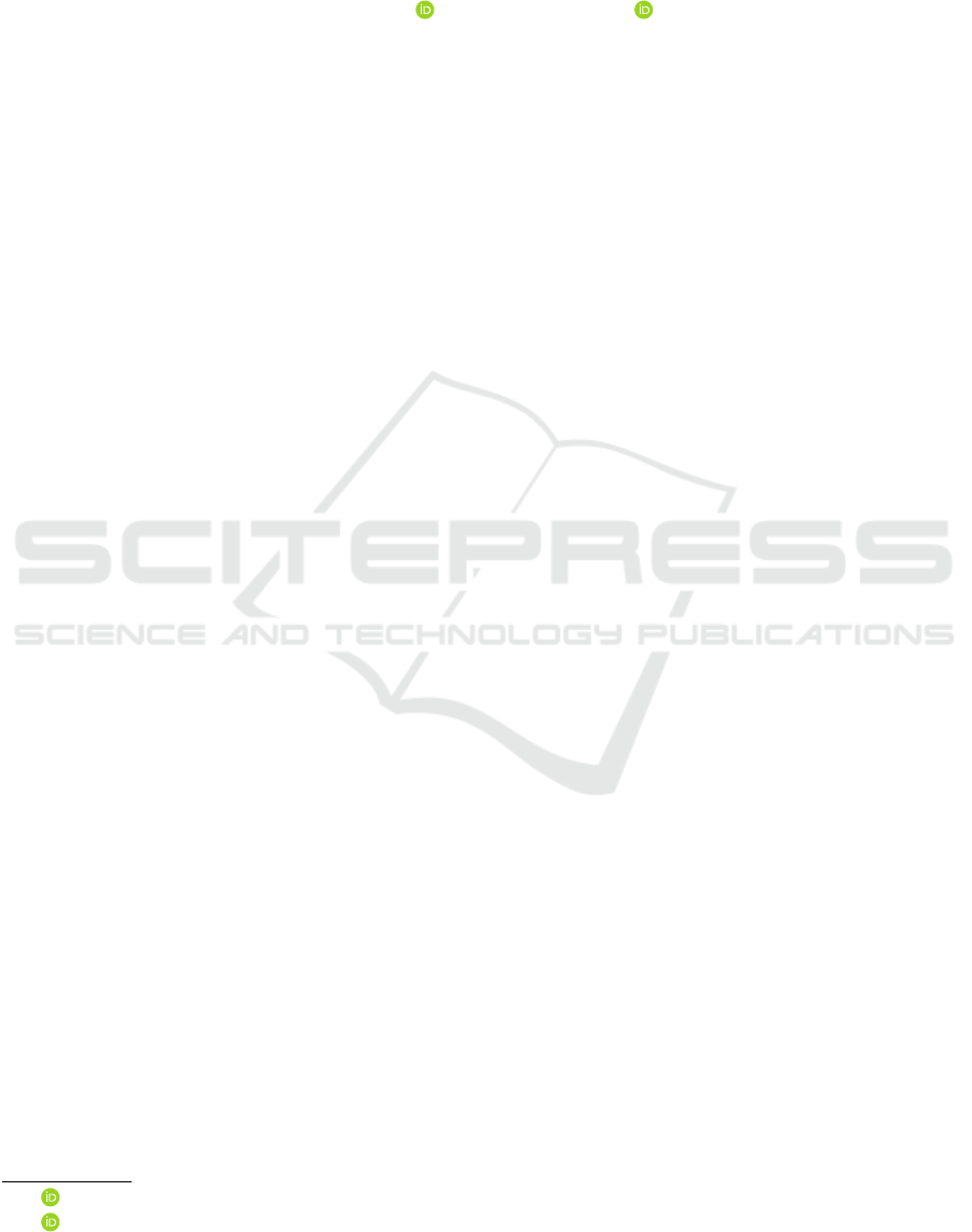
Figure 1 shows the overview of DG using SQ-

VAE. In Step 1, we divide N quantum vectors into

K groups, where N represents the number of quan-

tum vectors and K represents the number of cate-

gories. When an input feature is assigned to the quan-

tum vector deﬁned as category 0, the feature is pre-

dicted as category 0. In Step 2, we use ground truth

labels to group the features into K categories and train

the model to bring these groups of the same category

closer together. Step 3 is inference. Since we do not

have access to the target domain, a domain gap arises.

However, by aligning the groups of each category, we

can minimize the domain gap. Even if there is a gap

in the unseen target domain, the features of the target

domain are likely to be assigned to the same or simi-

lar quantum vectors as those in the source domain and

thus categorized similarly. By using these methods,

we can prevent accuracy degradation due to unseen

target domains.

Experiments were conducted to segment blood

vessels from retinal image datasets (Drive (J.Staal

et al., 2004), Stare (A.Hoover et al., 2000),

Chase (G.Jiaqi et al., )). Each dataset has a differ-

ent domain due to varying imaging devices. Two

retinal image datasets were used for training, while

the remaining one was utilized for evaluation. The

proposed method achieved an average improvement

of 1.36% in mIoU compared to the original U-Net

when it served as the feature extractor, with a no-

table average increase of 2.71% in vascular regions.

When we use UCTransNet as a feature extractor, the

proposed method improved mIoU by 1.02% over the

original UCTransNet, with a signiﬁcant improvement

of 2.17% in vascular regions.

Another experiment was conducted on

MoNuSeg (N.Kumar et al., 2020) dataset, which

exhibits diversity in nuclei across multiple organs

and patients and is captured under varying staining

methods at different hospitals. Therefore, DG is

required to extract features that are independent

of domain differences. Compared to the original

U-Net (O.Ronneberger et al., 2015), our method

using U-Net as a feature extractor improved mIoU by

2.53%, with an improvement of 2.73% in cell nuclei.

Additionally, compared to UCTransNet (H.Wang

et al., 2022), the proposed method using UCTransNet

as a feature extractor also improved mIoU by 3.0%,

with an improvement of 3.65% in cell nuclei.

The structure of this paper is as follows. Section 2

describes related works. Section 3 explains the details

of the proposed method. Section 4 presents and dis-

cusses the experimental results. Section 5 describes

conclusions and future work.

2 RELATED WORKS

2.1 Domain Generalization for

Semantic Segmentation

DG only allows access to the source domain and ex-

tracts features that are not speciﬁc to it (e.g., back-

ground or cell nuclei), mitigating domain shifts for

unseen target domains. Existing research on DG

for semantic segmentation often focuses on meth-

ods that remove domain-speciﬁc style information.

Techniques such as normalization (X.Pan et al.,

2018; S.Bahmani et al., 2022), whitening (S.Choi

et al., 2021), and diversiﬁcation (Y.Zhao et al., 2022;

D.Peng et al., 2021) have been used to achieve DG.

However, WildNet argued that style information and

content information are not orthogonal, and whiten-

ing style information can inadvertently remove nec-

Domain Generalization Using Category Information Independent of Domain Differences

369

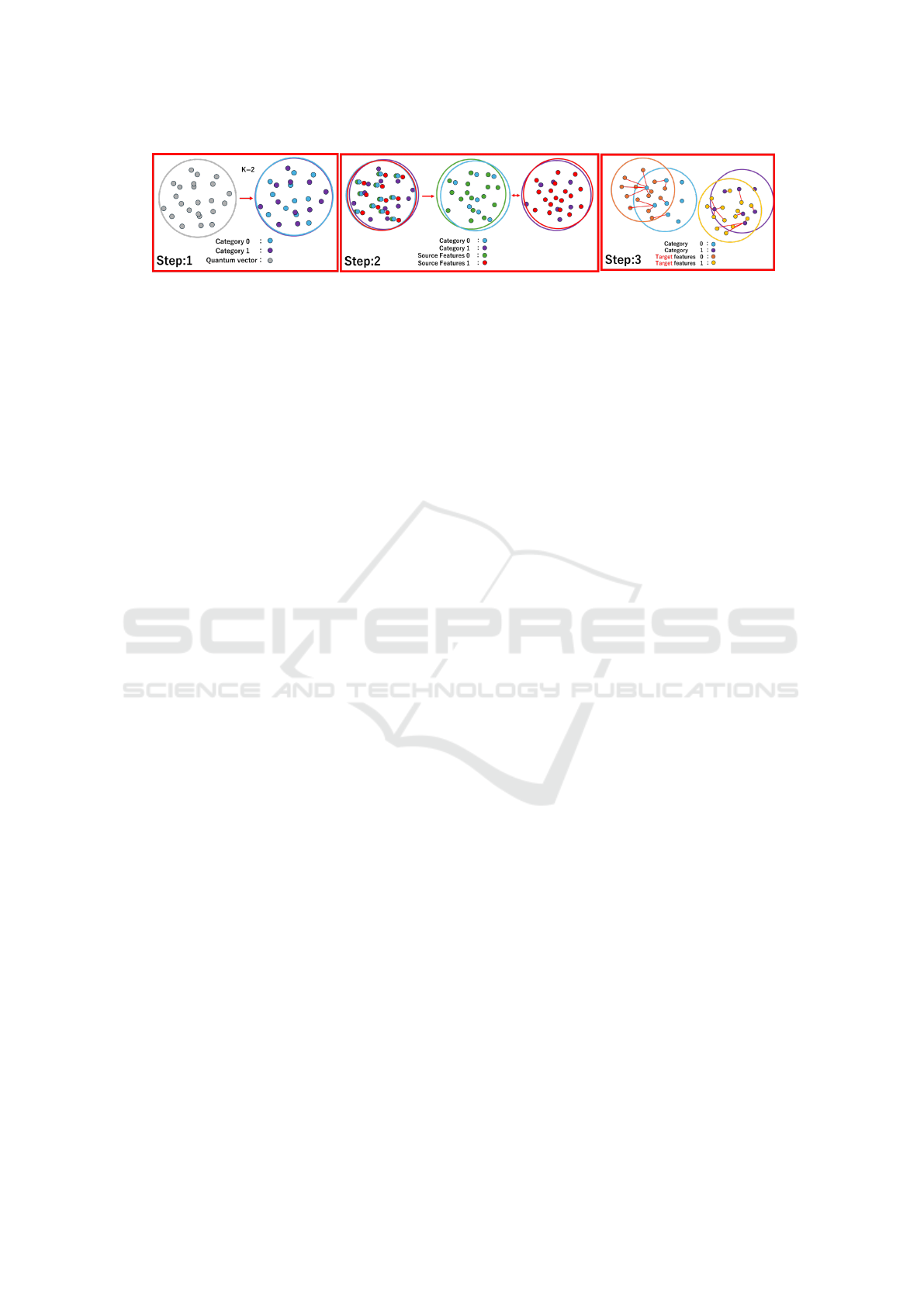
Figure 1: Overview of domain generalization using quantum vectors. This ﬁgure explains learning method for quantum

vectors used to absorb domain gaps and method to handle unseen target domains during inference.

essary content information. Therefore, to build a

high-precision model, it is essential to effectively ac-

quire information that is independent of the dataset.

We propose a method that splits the feature maps

from input images into two parts and trains them to

decorrelate from each other. One feature map is con-

strained to acquire category information independent

of domain differences, while the other retains source

domain-speciﬁc information. This approach allows

effective segmentation using feature maps that con-

tain category information independent of domain dif-

ferences.

2.2 Image Generation Model

Research on generative models has been extensive,

with various approaches proposed, such as Variational

Autoencoder (VAE) (Kingma and Welling, ), and

Vector Quantized VAE (VQ-VAE) (den Oord et al.,

2017). VAE maps input data to a latent space as a

probability distribution and samples latent variables

from this distribution to generate images. VQ-VAE

possesses higher quality image generation capabilities

and clustering abilities compared to VAE. However,

VQ-VAE has a non-differentiability issue due to the

use of the argmax function for discretization. This

problem was addressed by SQ-VAE. SQ-VAE uses

Gumbel-Softmax (E.Jang et al., 2016) to approximate

a categorical distribution in a differentiable manner,

allowing uninterrupted backpropagation. We propose

a method focusing on the clustering capability of SQ-

VAEs to bridge the domain gap between a source do-

main and an unseen target domain. Speciﬁcally, we

constrain the probabilities to divide the N quantum

vectors into K groups. Aligning the groups for each

category can minimize the gap with the unseen target

domain. This approach helps mitigate the accuracy

degradation caused by the target domain.

3 PROPOSED METHOD

When conventional semantic segmentation learns

from a speciﬁc dataset (source domain) and eval-

uates on an unseen dataset (target domain), accu-

racy decreases signiﬁcantly due to domain differ-

ences such as different imaging devices and stain-

ing methods. To improve accuracy through DG, we

propose two approaches. First, we separate feature

maps into domain-independent category information

and domain-speciﬁc information of the source do-

main. Using domain-independent category informa-

tion for segmentation, we believe that accuracy is in-

dependent of the dataset domain used for training.

Second, using only category information cannot com-

pletely bridge the domain gap between the source and

target domains. Therefore, we propose a method to

address the domain gap using the quantum vectors of

SQ-VAE.

3.1 Category Information Independent

of Domain Differences

Figure 2 illustrates the overview of our method. To

extract information independent of domain differ-

ences, an input image x ∈ R

3×H×W

is processed by

a feature extractor, such as U-Net or UCTransNet,

which outputs the feature map Z ∈ R

C×H×W

. The

feature extractor, such as U-Net or UCTransNet,

achieves high accuracy and provides output images

of the same dimensions as the input images. This is

why we use U-Net or UCTransNet as the encoder.

The feature maps obtained from the encoder are di-

vided along the channel dimension into two parts: the

domain-independent category information and the re-

maining information. The divided feature maps are

denoted as Z

∈ R

×H×W

and Z

∈ R

×H×W

where

= C

= C/2. To separate domain-independent cat-

egory information from source domain-speciﬁc infor-

mation, the model is trained to decorrelate the feature

maps Z

and Z

. In this paper, we adopt DeepCCA,

which can learn nonlinear relationships, allowing it to

handle more complex data and achieve high precision

in removing correlations.

DeepCCA maximizes the correlation between two

variables in a nonlinear manner. However, since our

goal is to decorrelate them, squaring the output of

ICPRAM 2025 - 14th International Conference on Pattern Recognition Applications and Methods

370

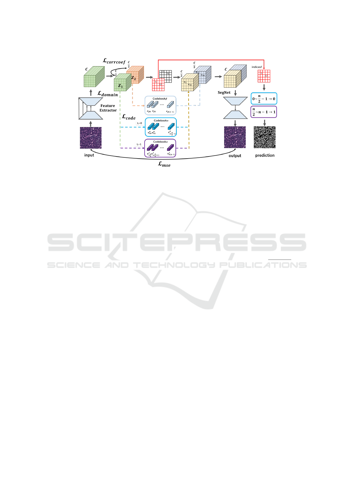
Figure 2: Overview of the proposed method. We extracted domain-independent category information to address unseen target

domains. Domain-independent category information is represented using Z

, which is used for segmentation. Additionally,

quantum vectors are used for quantization to bridge the gap between source domain and unseen target domain.

DeepCCA brings the result closer to zero.

corrcoe f

= corrcoe f (Z

)

(1)

After decorrelation, feature maps are quantized using

quantization vectors e

∈ R

N×C

and e

∈ R

N×C

. N

is the dimension of the embedding vector space. The

details are presented in Section 3.2. The reason for

preparing e

and e

is to assign them different roles.

is used to provide domain-independent categori-

cal features, while e

supplies source domain-speciﬁc

features. This approach allows each to serve distinct

functions. The feature maps after quantization are de-

noted as Z

′

and Z

′

. Z

′

and Z

′

are also trained to be

decorrelated using DeepCCA.

corrcoe f

= corrcoe f (Z

′

)

(2)

By using constraints in Equations 1 and 2, the

quantization vectors e

and e

become automatically

uncorrelated. By training Z

and Z

to be uncorre-

lated, they can assume different roles. For exam-

ple, if we assume that Z

and e

represent domain-

independent category features, then Z

and e

repre-

sent source domain-speciﬁc features. We hypothesize

that using these domain-independent features for seg-

mentation will improve accuracy. This method in-

volves training multiple features to be uncorrelated,

but there is no guarantee that Z

represents domain-

independent category information.

To address this, we propose a method to group fea-

tures within Z

that belong to the same category, em-

bedding domain-independent category information.

Speciﬁcally, we introduce a set of learnable represen-

tative vectors, t

∈ R

K×C

. Here, K denotes the num-

ber of categories. For example, for category t

, we

train the model to cluster features Z

in Z

with a tar-

get label of 0. This process is repeated for all K cat-

egories. Additionally, to ensure that these represen-

tative vectors do not capture source domain-speciﬁc

information, we train the model to separate the rep-

resentative vectors from each other. By doing so, we

can densely embed domain-independent category in-

formation.

domain

K−1

∑

i=0

||t

− Z

−

K−1

∑

j=0

||t

−t

(3)

where Z

and Z

are deﬁned as the features of Z

when the target label is 0 and 1.

3.2 Segmentation Using SQ-VAE

In Section 3.1, we proposed a method that divides

features into those related to domain-independent

categories and those speciﬁc to the source domain.

Although only domain-independent features provide

DG capabilities, this does not completely prevent the

domain gap. Thus, we propose a method to bridge the

domain gap between the source and unseen target do-

mains using quantum vectors from the SQ-VAE. The

reason for using SQ-VAE is that it can generate vari-

ous clusters by utilizing quantum vectors. Addition-

ally, SQ-VAE is more accurate as an image genera-

tion model compared to VAE and VQ-VAE. We con-

strain the N quantum vectors from the SQ-VAE into

K groups to address the domain gap. For instance,

in the category of cell nuclei, we train the model to

bring the group of quantum vectors representing cell

nuclei closer to the group of features obtained from

input images of cell nuclei. By aligning these groups,

Domain Generalization Using Category Information Independent of Domain Differences

371

we can mitigate the domain gap between the source

and unseen target domains, allowing for better gener-

alization. We feed an image x ∈ R

3×H×W

into the fea-

ture extractor, such as U-Net and UCTransNet, which

outputs a feature map Z ∈ R

C×H×W

. As explained in

Section 3.1, to separate domain-independent category

features from domain-speciﬁc features, we divide the

feature map into two parts: Z

and Z

To address the domain gap, we deﬁne the quan-

tum vectors as e ∈ R

N×C/2

where C/2 is the chan-

nel dimension of the embedded vector e. We sepa-

rate domain-independent category information from

domain-speciﬁc in e

∈ R

N×C

and e

∈ R

N×C

. To

quantize the feature map obtained from the feature

extractor, we calculate the Mahalanobis distance be-

tween the feature map Z

and the quantum vector e

logit

= −

α j

− Z

)

⊤

−1

α j

− Z

)

N−1

j=0

(4)

where Σ

is a learnable parameter, and j refers to one

of the quantum vectors within the set of N vectors. It

is denoted as

∑

= σ

I. Then, logit

is expressed as

logit

||e

α j

− Z

2σ

(5)

where logit

∈ R

HW ×N

is a matrix. In this case,

∑

I is learned to approach zero from the initial value.

As training progresses, the probabilities of the dis-

tances between feature maps obtained by the encoder

and the quantum vectors become closer to a one-hot

encoding. This is similar to SQ-VAE. To probabilisti-

cally quantify the Mahalanobis distance between the

obtained feature map and the quantum vectors, we use

Gumbel-Softmax. We use Gumbel-Softmax because

it approximates the selection of discrete quantum vec-

tors as a continuous probability distribution and is dif-

ferentiable.

= Gumbelsoftmax



−

logit



(6)

where τ is a learnable temperature parameter. Sim-

ilarly, we use Z

and e

to output P

. As shown in

Equations 5 and 6, we calculate the Mahalanobis dis-

tance and convert it to probabilities using Gumbel-

Softmax. These probabilities are then used to quan-

tize the features obtained from the encoder.

During evaluation, we replace the feature map ob-

tained from Equation 5 with the quantum vector that

has the closest Mahalanobis distance.

indices

= argmax(logit

) (7)

where argmax is used along the N-dimensional direc-

tion of logit

∈ R

HW ×N

The feature maps fed into the decoder are quan-

tized as Z

′

∈ R

×H×W

and Z

′

∈ R

×H×W

. Since the

channel dimension is split into two, the dimensions

from Z

′

and Z

′

are combined.

′

= Concat(Z

′

) (8)

According to Equation 8, it becomes Z

′

∈ R

C×H×W

The decoder shown in Figure 2 uses an encoder-

decoder CNN (V.Badrinarayanan et al., 2017) with-

out skips. This is because U-Net or UCTransNet fea-

tures transmission mechanisms that allow the input

image to ﬂow through easily, simplifying reconstruc-

tion and hindering the learning of intermediate layers.

The input Z

′

is passed through the encoder-decoder

CNN, producing the ﬁnal output x

′

. The reconstruc-

tion error between the input image x and the ﬁnal out-

put image x

′

is then calculated.

mse

∑

i=1

log(x

− x

′

)

(9)

where n is the total number of pixels in the input im-

age. The reason for adding log to the loss is that

the gradient becomes larger as x decreases. In other

words, we believe that the model should focus on ﬁner

details during reconstruction. This is consistent with

the implementation of SQ-VAE.

The objective is to use features related to cate-

gories that are independent of domain differences and

employ quantum vectors to prevent domain gaps for

unseen target domains. Additionally, segmentation is

performed by the indices of the quantum vectors. This

is executed using Z

and e

∈ R

N×C

. It is divided

into K parts to separate roles based on the number of

segmentation categories K.

In this paper, we consider the case where K=2.

First, it is divided into two parts: e

∈ R

×C

, corre-

sponding to category label 0, and e

∈ R

×C

, cor-

responding to category label 1. Let N

and N

such that N

= N

= N/2. From Equation 6, we have

∈ R

H×W ×N

. When the category label is 0, we want

the probability of selecting e

to be 1. Similarly, when

the category label is 1, we want the probability of se-

lecting e

to be 1. To achieve this, we train the model

such that the sum of probabilities in the N

dimen-

sional direction of P

is 1 when the category label is

0, and the sum of probabilities in the N

dimensional

direction of P

is 1 when the category label is 1. In

other words, when the category label is 0, the model is

trained to minimize the distance between the feature

map Z

∈ R

×H

×W

related to the category label and

∈ R

×C

where H

and W

correspond to category

label 0. When the category label is 1, the model is

trained to minimize the distance between the feature

map Z

∈ R

×H

×W

related to the category label and

∈ R

×C

where H

and W

correspond to category

ICPRAM 2025 - 14th International Conference on Pattern Recognition Applications and Methods

372

Figure 3: Weights that are learned to focus on parts where

predictions become uncertain. Treat red as weight.

label 1. This learning method is as

code

= log

× (1 −

−1

∑

N=0

)

L=0

× (1 −

N−1

∑

)

L=1

(10)

where L is the label, and w

and w

are weights added

to prioritize uncertain predictions. By using these

weights, the model can focus on learning parts where

predictions are uncertain, such as the boundaries in

segmentation.

Figure 3 shows a conceptual diagram of the

weights. The maximum values of the prediction prob-

abilities from index 0 to (N-1)/2 and from N/2 to N-

1 are obtained. These are deﬁned as max(P

) and

max(P

), respectively. Next, the absolute value of the

difference between these maximum values is taken as

di f = |max(P

) − max(P

)| (11)

The absolute differences are collected for all pixels

and divided by the maximum value among all pixels

to normalize them from 0 to 1. The weight of the i-th

pixel is as follows:

di f

max(di f )

(12)

The weight w is less likely to be learned if it is closer

to 1, as it indicates higher certainty. Conversely, if it is

closer to 0, it signiﬁes greater uncertainty in the pre-

diction, and it is learned more intensively. The reason

weights closer to 0 are learned more intensively than

those closer to 1 is that Equation 10 includes a log,

making smaller loss values more signiﬁcant. Taking

the derivative of log(x) results in 1/x, meaning that

as x becomes smaller, the gradient becomes larger,

thereby making smaller loss more signiﬁcant.

Finally, the index of the quantization vector clos-

est to the feature vector is obtained, which is related

to the category and independent of the domain dif-

ferences. If this index is between 0 and (N/2) − 1,

category label 0 is assigned. If the index is between

N/2 and N −1, category label 1 is assigned. This cat-

egory label is used as the ﬁnal segmentation predic-

tion. The learning method using this quantized vector

is shown in Figure 1, with Step 2 particularly pertain-

ing to that part. When the category label is 0, the

model is trained so that the sum in the N

dimensional

direction of P

equals 1. When the category label is 1,

the model is trained so that the sum in the N

dimen-

sional direction of P

equals 1. This approach divides

the features into two groups using the labeled data,

similar to dividing the quantization vectors into two

groups. The model is then trained to bring the groups

closer together. As a result, even in the presence of a

domain gap in the unseen target domain, it can be mit-

igated, as quantization assigns similar quantum vec-

tors to clusters (groups of the same category).

4 EXPERIMENTS

4.1 Implementation Details

Our method is evaluated on blood vessel segmenta-

tion from three types of fundus images: Drive, Stare,

and Chase. The Drive, Stare, and Chase datasets each

contain a total of 20, 20, and 28 images, respectively,

along with annotations for segmenting the images into

classes: background and blood vessels. The images

in the Drive dataset were captured using a Canon CR5

non-mydriatic 3CCD camera. The images in the Stare

dataset were obtained using a Top Con TRV-50 reti-

nal camera. The images in the Chase dataset were

captured with a Nidek NM-200-D fundus camera. As

these images were taken with different cameras, they

can be considered to belong to different domains.

Of the three datasets, two are used for training,

while the remaining dataset is used for evaluation. By

rotating this arrangement, the DG performance is as-

sessed. Each dataset is divided into ﬁve parts to per-

form 5-fold cross-validation, with four parts used for

training (e.g., 4/5 of Drive and 4/5 of Chase) and one

part used for validation (e.g., 1/5 of Drive and 1/5 of

Chase). Subsequently, the two datasets used for train-

ing and validation are combined to ensure there is no

data imbalance. The validation data from the remain-

ing dataset, which was not used for training, is used

for evaluation (e.g., 1/5 of Stare). However, since the

Chase dataset contains more images, to avoid bias in

training or evaluation, the number of images in the

Chase dataset is randomly reduced to 20 for the ex-

periments.

Additionally, we conduct experiments on the

MoNuSeg dataset, which contains tissue images of

tumors from various organs diagnosed in several pa-

tients across multiple hospitals. Due to the diverse

appearance of nuclei across different organs and pa-

tients, as well as the variety of staining methods

used by various hospitals, it is important to extract

domain-agnostic information from this dataset. The

Domain Generalization Using Category Information Independent of Domain Differences

373

MoNuSeg dataset consists of 30 images for training

and 14 images for evaluation. Among the training

data, 24 images are allocated for training, and 6 im-

ages are reserved for validation. The test data is used

as is for evaluation and includes lung and brain cells

that are not present in the training data, rendering

them unseen data.

For all experiments, the seed value is changed four

times to calculate average accuracy. We resize all im-

ages to 256 × 256 pixels as preprocessing. The learn-

ing rate is set to 1 × 10

−3

, the batch size is 2, the op-

timizer is Adam, and the number of epochs is 200.

We used an Nvidia RTX A6000 GPU. The number of

quantum vectors is set to 512. The evaluation metric

is intersection over union (IoU), and we evaluate us-

ing the IoU for each class and the mean IoU (mIoU)

across all classes. We compared the proposed method

with U-Net and UCTransNet. The rationale is that the

proposed method uses U-Net or UCTransNet as an

encoder and makes predictions using quantum vectors

based on its output. In other words, the same feature

extractor is used up to the point of segmentation pre-

diction.

4.2 Domain Generalization on Chase,

Stare, and Drive Datasets

The results of DG on the Chase, Stare, and Drive

datasets are shown in Table 1. The method with

the highest accuracy is shown in orange, while the

second-highest accuracy is in blue. When the Drive

and Stare datasets were used for training and the

Chase dataset for evaluation, the proposed method

(U-Net+ours) using U-Net as a feature extractor ex-

hibited a 1.80% improvement in mIoU compared

to the original U-Net, with a speciﬁc improvement

of 3.69% in the blood vessel area. Additionally,

the proposed method (UCTransNet+ours) using UC-

TransNet as a feature extractor demonstrated a 2.41%

improvement in mIoU compared to the original UC-

TransNet, with a speciﬁc improvement of 5.01% in

the blood vessel area. When the Drive and Chase

datasets were used for training and the Stare dataset

for evaluation, the proposed method (U-Net+ours) us-

ing U-Net as a feature extractor showed a 1.20% im-

provement in mIoU compared to the original U-Net,

with a speciﬁc improvement of 2.47% in the blood

vessel area. Additionally, the proposed method (UC-

TransNet+ours) using UCTransNet as a feature ex-

tractor noted a 0.32% improvement in mIoU com-

pared to the original UCTransNet, with a speciﬁc im-

provement of 0.76% in the blood vessel area. When

the Stare and Chase datasets were used for training

and the Drive dataset for evaluation, the proposed

Table 1: IoU and standard deviation Chase, Stare, and Drive

datasets. orange indicates the highest accuracy, and blue

indicates the second-highest accuracy.

datasets methods background blood vessels mIoU

Chase

U-Net 95.33(±0.35) 43.56(±4.14) 69.44(±2.15)

U-Net + ours 95.24(±0.48) 47.25(±1.82) 71.24(±1.13)

UCTransNet 95.27(±0.37) 45.92(±3.84) 70.59(±1.97)

UCTransNet + ours 95.06(±0.39) 50.93(±1.65) 73.0(±0.92)

Stare

U-Net 95.81(±0.86) 56.70(±6.79) 76.26(±3.73)

U-Net + ours 95.75(±0.71) 59.17(±4.16) 77.46(±2.36)

UCTransNet 95.80(±0.85) 56.71(±5.66) 76.25(±3.20)

UCTransNet + ours 95.67(±0.71) 57.47(±4.17) 76.57(±2.36)

Drive

U-Net 95.56(±0.53) 57.86(±1.85) 76.71(±1.17)

U-Net + ours 95.75(±0.40) 59.84(±3.06) 77.80(±1.57)

UCTransNet 95.62(±0.49) 58.35(±2.10) 76.99(±1.28)

UCTransNet + ours 95.58(±0.46) 59.10(±1.58) 77.34(±1.01)

method (U-Net+ours) using U-Net as a feature ex-

tractor showed a 1.09% improvement in mIoU com-

pared to the original U-Net, with a speciﬁc improve-

ment of 1.98% in the blood vessel area. Addition-

ally, the proposed method (UCTransNet+ours), using

UCTransNet as a feature extractor showed a 0.35%

improvement in mIoU compared to the original UC-

TransNet, with a speciﬁc improvement of 0.75% in

the blood vessel area. These improvements indicate

that DG is effectively achieved.

Additionally, segmentation results are shown in

Figure 4. The top three rows display the results on

the Chase, Stare, and Drive datasets. The areas high-

lighted in red boxes show signiﬁcant improvements.

For the Chase dataset, vascular regions in the red

box of the input image appear slightly darker, which

the original U-Net and UCTransNet predict as back-

ground. In contrast, our methods (U-Net+ours and

UCTransNet+ours) extract category information in-

dependently of the domain, preventing domain gaps,

can densely extract blood vessel category informa-

tion, predicting them correctly. For the Stare dataset,

focusing on the red box areas, the original U-Net

and UCTransNet make predictions indicating discon-

nected blood vessels. However, the proposed meth-

ods (U-Net+ours and UCTransNet+ours) predict con-

nected blood vessels, effectively extracting category

information independently of the domain. For the

Drive dataset, in the red box areas, the original U-

Net and UCTransNet predict the blood vessels as thin

or disconnected. In contrast, the proposed methods

predict thicker blood vessels and connect previously

disconnected vessels, successfully extracting domain-

independent information.

4.3 Domain Generalization on

MoNuSeg

The results of DG on the MoNuSeg dataset are shown

in Table 2. The method with the highest accuracy

is highlighted in orange, while the method with the

second-highest accuracy is shown in blue. Compar-

ICPRAM 2025 - 14th International Conference on Pattern Recognition Applications and Methods

374

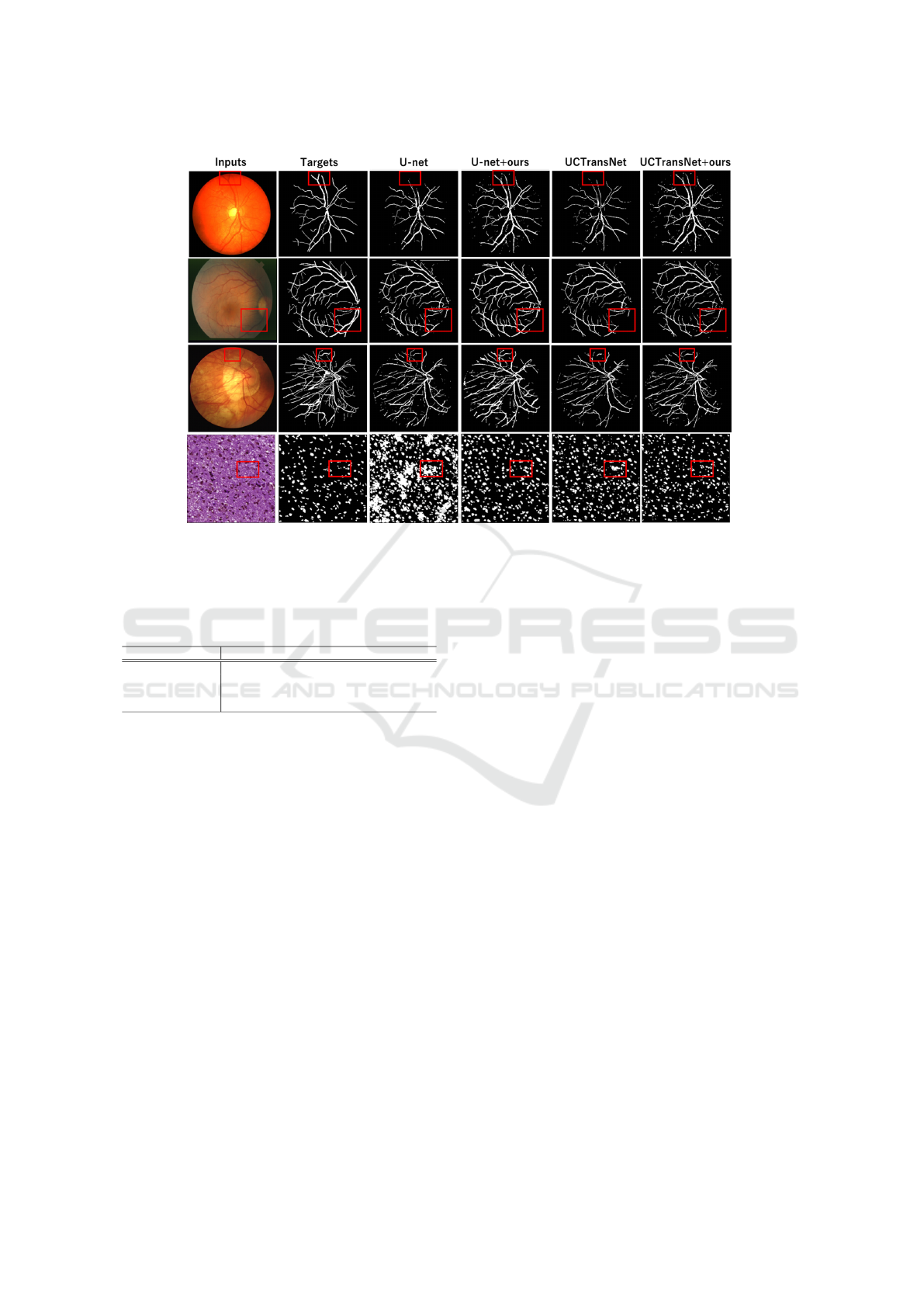
Figure 4: Segmentation results on Chase, Stare, MoNuSeg, and Drive datasets. From left to right, the images show input

images, ground truth, results by original U-Net, our method (U-Net+ours), original UCTransNet, and our method (UC-

TransNet+ours).

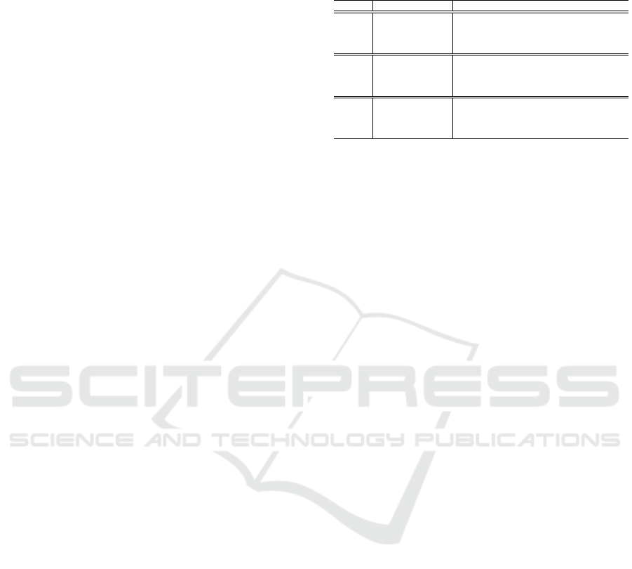
Table 2: IoU and standard deviation on MoNuSeg dataset.

orange method achieved the highest accuracy, while blue

method attained the second-highest accuracy.

methods background cell nucleus mIoU

U-Net 87.36(±0.96) 61.55(±1.17) 74.46(±1.01)

U-Net + ours 89.71(±1.24) 64.28(±1.10) 76.99(±1.17)

UCTransNet 87.79(±0.07) 60.93(±0.51) 74.36(±0.23)

UCTransNet + ours 90.15(±0.95) 64.58(±0.67) 77.36(±0.80)

ison results between conventional methods and the

proposed methods (methods + ours) are included. As

a result, the proposed method (U-Net+ours) achieved

a 2.53% improvement in mIoU compared to the orig-

inal U-Net, with a speciﬁc improvement of 2.73%

in the cell nucleus area. Additionally, the pro-

posed method (UCTransNet+ours) achieved a 3.0%

improvement in mIoU compared to the original UC-

TransNet, with a speciﬁc improvement of 3.65% in

the cell nucleus area. These results demonstrate

strong generalization performance to unseen target

domains. The improved accuracy in cell nuclei, in

particular, suggests that the method can effectively

handle the diversity in the appearance of cell nuclei

and staining methods across different domains, suc-

cessfully extracting cell nucleus-speciﬁc features.

Segmentation results from conventional methods

and our methods are displayed in the bottom row of

Figure 4. The areas highlighted in red boxes indicate

where signiﬁcant improvements were observed. The

original U-Net struggled with DG, often predicting

background as cell nuclei. In contrast, the proposed

method (U-Net+ours) successfully extracted category

information independent of the domain, closing do-

main gaps and enabling accurate predictions. Simi-

larly, the original UCTransNet over-predicted cell nu-

clei in the areas highlighted in red. However, the

proposed method (UCTransNet+ours) effectively ex-

tracted information on various cell nuclei, leading to

accurate predictions.

5 CONCLUSION

We proposed a method that generalizes well to

datasets with differences in imaging equipment and

staining methods (target domain) compared to the

dataset (source domain) on which the model was

trained. The proposed method showed signiﬁcant im-

provements on cell image datasets with various stain-

ing methods and fundus images captured by different

imaging devices. These results demonstrate the gen-

eralization performance of our method to unseen tar-

get domains. In the future, we would like to evaluate

our method on a multi-class segmentation problem.

ACKNOWLEDGMENTS

This paper is partially supported by the Strategic In-

novation Creation Program.

Domain Generalization Using Category Information Independent of Domain Differences

375

REFERENCES

A.Hoover et al. (2000). Locating blood vessels in retinal

images by piece-wise threshold probing of a matched

ﬁlter response. IEEE Transactions on Medical Imag-

ing, 19(3):203–210.

B.Cheng et al. (2022). Masked-attention mask transformer

for universal image segmentation. In Proceedings

of the IEEE/CVF conference on computer vision and

pattern recognition, pages 1290–1299.

den Oord, A. et al. (2017). Neural discrete representation

learning. In I.Guyon et al., editors, Advances in Neu-

ral Information Processing Systems, volume 30. Cur-

ran Associates, Inc.

D.Peng et al. (2021). Global and local texture random-

ization for synthetic-to-real semantic segmentation.

IEEE Transactions on Image Processing, 30:6594–

6608.

E.Jang et al. (2016). Categorical reparameterization with

gumbel-softmax. arXiv preprint arXiv:1611.01144.

F.Milletari et al. (2016). V-net: Fully convolutional neural

networks for volumetric medical image segmentation.

In 2016 fourth international conference on 3D vision

(3DV), pages 565–571. Ieee.

Furukawa, R. and Hotta, K. (2021). Localized feature ag-

gregation module for semantic segmentation. In 2021

IEEE International Conference on Systems, Man, and

Cybernetics (SMC), pages 1745–1750. IEEE.

G.Andrew et al. (2013). Deep canonical correlation analy-

sis. In Dasgupta, S. and McAllester, D., editors, Pro-

ceedings of the 30th International Conference on Ma-

chine Learning, volume 28 of Proceedings of Machine

Learning Research, pages 1247–1255, Atlanta, Geor-

gia, USA. PMLR.

G.Jiaqi et al. Chase: A large-scale and pragmatic chinese

dataset for cross-database context-dependent text-to-

sql.

H.Wang et al. (2022). Uctransnet: rethinking the skip

connections in u-net from a channel-wise perspective

with transformer. In Proceedings of the AAAI con-

ference on artiﬁcial intelligence, volume 36, pages

2441–2449.

J.Staal et al. (2004). Ridge-based vessel segmentation in

color images of the retina. IEEE transactions on med-

ical imaging, 23(4):501–509.

J.Wang et al. (2020). Deep high-resolution representa-

tion learning for visual recognition. IEEE transac-

tions on pattern analysis and machine intelligence,

43(10):3349–3364.

Kingma, D. P. and Welling, M. Auto-encoding variational

bayes.

N.Kumar et al. (2020). A multi-organ nucleus segmentation

challenge. IEEE Transactions on Medical Imaging,

39(5):1380–1391.

O.Ronneberger et al. (2015). U-net: Convolutional

networks for biomedical image segmentation. In

Medical Image Computing and Computer-Assisted

Intervention–MICCAI 2015: 18th International Con-

ference, Munich, Germany, October 5-9, 2015, Pro-

ceedings, Part III 18, pages 234–241. Springer.

P.Wang et al. (2023). One-peace: Exploring one gen-

eral representation model toward unlimited modali-

ties. arXiv preprint arXiv:2305.11172.

S.Bahmani et al. (2022). Semantic self-adaptation: Enhanc-

ing generalization with a single sample. arXiv preprint

arXiv:2208.05788.

S.Choi et al. (2021). Robustnet: Improving domain gen-

eralization in urban-scene segmentation via instance

selective whitening. In Proceedings of the IEEE/CVF

conference on computer vision and pattern recogni-

tion, pages 11580–11590.

Shibuya, E. and Hotta, K. (2020). Feedback u-net for cell

image segmentation. In Proceedings of the IEEE/CVF

Conference on computer vision and pattern recogni-

tion workshops, pages 974–975.

S.Lee et al. (2022). Wildnet: Learning domain generalized

semantic segmentation from the wild. In Proceedings

of the IEEE/CVF conference on computer vision and

pattern recognition, pages 9936–9946.

V.Badrinarayanan et al. (2017). Segnet: A deep convo-

lutional encoder-decoder architecture for image seg-

mentation. IEEE transactions on pattern analysis and

machine intelligence, 39(12):2481–2495.

X.Pan et al. (2018). Two at once: Enhancing learning

and generalization capacities via ibn-net. In Proceed-

ings of the european conference on computer vision

(ECCV), pages 464–479.

Y.Liu et al. (2020). Efﬁcient semantic video segmentation

with per-frame inference. In Computer Vision–ECCV

2020: 16th European Conference, Glasgow, UK, Au-

gust 23–28, 2020, Proceedings, Part X 16, pages 352–

368. Springer.

Y.Takida et al. (2022). SQ-VAE: Variational Bayes on

discrete representation with self-annealed stochastic

quantization. In Chaudhuri, K., Jegelka, S., Song,

L., Szepesvari, C., Niu, G., and Sabato, S., edi-

tors, Proceedings of the 39th International Conference

on Machine Learning, volume 162 of Proceedings

of Machine Learning Research, pages 20987–21012.

PMLR.

Y.Zhao et al. (2022). Style-hallucinated dual consistency

learning for domain generalized semantic segmenta-

tion. In European conference on computer vision,

pages 535–552. Springer.

ICPRAM 2025 - 14th International Conference on Pattern Recognition Applications and Methods

376