
Curvy: A Parametric Cross-Section Based Surface Reconstruction
Aradhya N. Mathur
a
, Apoorv Khattar and Ojaswa Sharma
b
Indraprastha Institute of Information Technology Delhi, India
Keywords:
Graph Neural Networks, Parametric Representation, Shape Reconstruction.
Abstract:
In this work, we present a novel approach for reconstructing shape point clouds using planar sparse cross-
sections with the help of generative modeling. We present unique challenges pertaining to the representation
and reconstruction in this problem setting. Most methods in the classical literature lack the ability to gener-
alize based on object class and employ complex mathematical machinery to reconstruct reliable surfaces. We
present a simple learnable approach to generate a large number of points from a small number of input cross-
sections over a large dataset. We use a compact parametric polyline representation using adaptive splitting to
represent the cross-sections and perform learning using a Graph Neural Network to reconstruct the underlying
shape in an adaptive manner reducing the dependence on the number of cross-sections provided.
Project page: https://graphics-research-group.github.io/curvy/.
1 INTRODUCTION
Surface reconstruction from cross-sections is a well-
explored problem (Huang et al., 2017; Memari and
Boissonnat, 2008; Boissonnat and Memari, 2007; Ba-
jaj et al., 1996). There is a rich literature on methods
demonstrating the generation of reliable surfaces from
cross-sections for several applications. Medical imag-
ing and industrial manufacturing are some fields that
require reconstruction from such data. Little work ex-
ists that provides insights into how complex objects
could be generated using cross-sections with the help
of deep learning methods that could provide an added
advantage of capturing the semantic context associ-
ated with shapes. Deep learning-based methods (Sar-
mad et al., 2019; Park et al., 2019) can provide bet-
ter generalizability qualities associated with unseen
shapes of similar types by learning associated latent
representations. Several methods have extensively ex-
plored surface reconstruction from other inputs such
as point clouds (Brüel-Gabrielsson et al., 2020; Kazh-
dan et al., 2006; Peng et al., 2021). Inspired by these
two primary directions we aim to solve the task of
point cloud reconstruction from cross-sections unlike
the well-explored problem of surface generation from
incomplete point clouds. This brings unique chal-
lenges that we aim to address in this paper. Given the
proven effectiveness of deep learning in point cloud
a
https://orcid.org/0000-0001-6141-5849
b
https://orcid.org/0000-0002-9902-1367
generation, we leverage these methods to generate 3D
point clouds that can subsequently be used for surface
reconstruction, as extensively explored in prior work.
Thus, our focus is on the generation of high-quality
point clouds from sparse unorganized cross-sections.
Previous approaches for point cloud completion have
focused on generating point clouds from images or
representation learning using autoencoders. Several
previous methods focused on generating surfaces us-
ing cross-sections and did not involve any learning
based on the class of objects. Our method can be
used with any modern encoder-decoder-based point
cloud generation since it focuses on learning the latent
embeddings rather than generating the point cloud di-
rectly. Our approach introduces a novel input repre-
sentation for the cross-sections, aiming to capture cru-
cial information that would be overlooked when using
surface-sampled points. Point clouds, while dense in
most areas, often suffer from incomplete information
in certain regions. In contrast, cross-section curves
exhibit a highly non-uniform distribution of informa-
tion, necessitating reconstruction methods capable of
handling sparse and anisotropic data. By consider-
ing this unique characteristic of cross-sections, our
approach enables a more comprehensive and accurate
reconstruction of shapes. Our contributions can be
summarised as follows:
1. An approach for learning surface reconstruc-
tion based on parametric representation of cross-
sections for reconstruction,
Mathur, A. N., Khattar, A. and Sharma, O.
Curvy: A Parametric Cross-Section Based Surface Reconstruction.
DOI: 10.5220/0013300500003912
Paper published under CC license (CC BY-NC-ND 4.0)
In Proceedings of the 20th International Joint Conference on Computer Vision, Imaging and Computer Graphics Theory and Applications (VISIGRAPP 2025) - Volume 1: GRAPP, HUCAPP
and IVAPP, pages 139-150
ISBN: 978-989-758-728-3; ISSN: 2184-4321
Proceedings Copyright © 2025 by SCITEPRESS – Science and Technology Publications, Lda.
139

2. A novel framework for generating a point cloud
while adapting to the anisotropic and sparse na-
ture of input cross-sections. This constitutes two
attention mechanisms to focus on the local and
global structure of the cross-sections and show
their significance empirically through an ablation
study, and
3. A new dataset for parametric representation of
cross-sections. The script for generating the
dataset shall be provided with the source code re-
lease.
2 RELATED WORK
Surface reconstruction is a widely studied problem in
computer graphics. As methods for representing 3D
data change, so do the methods for shape reconstruc-
tion. The different methods for representing 3D data
include a voxel-based representation that gives infor-
mation pertaining to points in a discrete grid, point
clouds that contain the locations of information, and
meshes that have added neighborhood information in
the form of an adjacency matrix corresponding to the
points. Newer implicit methods directly target surface
generation by learning to produce the implicit field
functions. We divide this section based on the repre-
sentation of the output for different methods.
2.1 Pointcloud Generation
There are two primary approaches that have been ex-
plored for point cloud reconstruction. Reconstruc-
tion of point clouds has been done using multi-
view/single-view images and partial-point clouds.
A deep autoencoder network for the reconstruc-
tion of point clouds results in compact representations
and can perform semantic operations, interpolations,
and shape completion (Achlioptas et al., 2018),(Lin
et al., 2018). These networks leverage 1-D and 2-
D convolutional layers to extract latent representa-
tion for the generation of point clouds. Single im-
age point cloud generation has also been performed
hierarchically from low resolution by gradually up-
sampling the point cloud as explored in (Fan et al.,
2017). This multi-stage process uses EMD distance
(Fan et al., 2017) and computes Chamfer distance
for the later stages w.r.t. ground truth dense point
cloud. Another approach uses multi-resolution tree-
structured network that allows to process point clouds
for 3D shape understanding and generation (Gadelha
et al., 2018). Some newer methods also approach this
problem from a local supervision perspective to un-
derstand the local geometry better (Han et al., 2019).
Further, skip-attention has shown to play an impor-
tant role in tasks such as point cloud completion
(Wen et al., 2020). The architecture proposed con-
sists of primarily three parts - a point cloud encoder,
a decoder that generates the point cloud, and skip-
attention layers that fuse relevant features from the
encoder to the decoder at different resolutions. Rein-
forcement learning has also been explored with GANs
trained for the point cloud generation. The agent is
trained for predicting a good seed value for the ad-
versarial reconstruction of incomplete point clouds
(Sarmad et al., 2019). The method uses an autoen-
coder trained on complete point clouds to generate
the global feature vector (GFV) and a GAN that is
trained to produce GFV. The pipeline uses GFV gen-
erated from an incomplete point cloud as a state and
supplies it to an RL agent which the GAN uses to
generate GFV close to the GFV of a complete point
cloud.
2.2 Surface Reconstruction
One of the seminal works (Memari and Boisson-
nat, 2008) proposes constructing 2D geometric shapes
from 1D cross-sections. The method provides sam-
pling conditions to guarantee the correct topology
and closeness to the original shape for the Haus-
dorff distance. One of the early works (Huang
and Menq, 2002) proposes a manifold mesh recon-
struction method from unorganized points with arbi-
trary topology. The method proposed defines a two-
step process for reliably reconstructing the geometric
shape from unorganized point cloud sampled from its
surface.
Early works took inspiration from medical imag-
ing problems, a two-step process for the reconstruc-
tion of a surface from cross-sections has been pro-
posed by first computing the arrangement for the
cross-section within each cell and then reconstruct-
ing an approximation of the object from its intersec-
tion with the cell boundary and gluing the pieces back
together yields to surface (Boissonnat and Memari,
2007). An algorithm for non-parallel cross-sections
consisting of curve networks of arbitrary shape and
topology has also been developed (Liu et al., 2008).
Several methods propose implicit field-based recon-
struction. One such method utilizes sign agnostic
learning for geometric shapes (Atzmon and Lipman,
2020). This method uses a deep learning-based ap-
proach that allows learning of implicit shape repre-
sentations directly from unsigned raw data like point
clouds and triangle soups. The proposed unsigned
distance loss family possesses plane reproduction
property based on suitable initialization of the net-
work weights.
GRAPP 2025 - 20th International Conference on Computer Graphics Theory and Applications
140

The surface reconstruction method has been per-
formed with topological constraints (Lazar et al.,
2018). The method relies on computing candidates
for cell partitioning of ambient volume. The method
is based on the calculation of a single surface patch
per cell so that the connected manifold surface of
some topology is obtained. 3D surface reconstruc-
tion from unorganized planar cross-sections using a
split-merge approach using Hermite mean-value in-
terpolation for triangular meshes has also been used
(Sharma and Agarwal, 2017). A divide-and-conquer
optimization-based strategy can also be employed
to perform topology-constrained reconstruction (Zou
et al., 2015). New methods like Orex (Sawdayee
et al., 2022) leverage deep learning for cross-section
to surface generation.
3 APPROACH
In this work, we develop an approach for shape re-
construction from a set of unorganized cross-sections.
We design a deep neural network that learns the over-
all structure of various shapes and generates a point
cloud representing the original object. Our approach
can be defined as a three-step process. We first gener-
ate a large number of cross-sections from 3D models
and sample them to create input cross-sectional data.
Then surface points are sampled to generate a point
cloud on which an autoencoder is trained to recon-
struct the point cloud. In the final step, we use the en-
coded vector obtained from the autoencoder and train
a Graph Neural Network on the parametric represen-
tation of input cross-sections to generate an embed-
ding vector in a GAN-based setting to match the en-
coded vector for the same object. These embedding
vectors are then decoded to get a point cloud from the
pre-trained autoencoder network.
Cross-section-based reconstruction has applica-
tions in several domains such as the manufacturing
of 3D components and 3D printing using CAD mod-
eling, and the medical domain where 2D ultrasound
slices are captured in 3D. Instead of sampling points
from the cross-sections, we convert an entire cross-
section curve into its parametric representation which
is a more versatile representation as it allows us to
reduce any loss of information that may occur due
to sampling and further helps reduce the memory re-
quirements needed to represent a large number of
points in the neural network, thus helping to capture
complex curves using fewer parameters. Let us as-
sume the density of points ρ per unit length of a cross-
section curve of length l. Depending on the sampling
density ρ, the number of points in a curve can vary,
and for better information capture we need a high ρ
value to capture the curvature accurately. We note that
the parametric curve can be represented using a fixed
number of coefficients from which any arbitrary den-
sity of points can be sampled. Our overall approach
is shown in Figure 1.
3.1 Adaptive Splitting
It is important to ensure that a simpler piece (such
as a straight line) is represented by fewer points so
that more points can be assigned to a piece with
many sharp turns. We propose an adaptive splitting
scheme for non-uniform distribution between pieces
using the Douglas-Peucker polyline simplification al-
gorithm (Douglas and Peucker, 1973) for finding a set
of endpoints to generate the pieces within the curve.
This helps to save more points for complex curves and
uses fewer points for simpler curves further retain-
ing more information than a uniform splitting scheme.
Douglas-Peucker algorithm is run for multiple iter-
ations till the final number of unique endpoints re-
turned is more than k, we select the k points with max-
imum absolute angle, where the angle varies between
−90 and +90. Each cross-section is divided into k
pieces using an adaptive splitting scheme. For the j
th
piece with n
j
points, we obtain the parameter values
of the parametric function using the Chordal approxi-
mation (Floater and Surazhsky, 2006) as,
t
i, j
= t
i−1, j
+
||p
i, j
− p
i−1, j
||
2
n
j
∑
i=2
||p
i, j
− p
i−1, j
||
2
,
where p
i
for i ∈ 1, 2, ...n
j
are points on a piece, and
t
1
= 0 such that for each piece t
i
∈ [0, 1]. Once we
have obtained k pieces, we fit piece-wise polynomi-
als by solving the KKT conditions (Kuhn and Tucker,
2014) by formulating a least squares problem (Boyd
and Vandenberghe, 2018).
3.2 Training on Parametric Space
We take the ShapeNet dataset (Chang et al., 2015) and
use the manifold meshes. The input cross-sections
are generated using mesh-plane intersection and con-
verted to parametric representation. Further in the
text, cross-sections shall refer to the parametric repre-
sentation of cross-sections. We sample surface points
from the meshes; thus, each set of cross-sections and
the corresponding point clouds form the input and the
corresponding ground truth for the network. In order
to use parameters with a neural network there are cer-
tain properties that the operations on the parametric
Curvy: A Parametric Cross-Section Based Surface Reconstruction
141

Input cross-sections
Piece-level graph
Graph
convolutions
Graph
convolutions
Point cloud
decoder
Generated point cloud
Figure 1: Overview of our reconstruction approach. Starting from a parametric representation of the given cross-sections, we
train a network to generate a surface point cloud.
representation must possess. Each piece of a cross-
section is represented as a tensor in R
6×3
of coeffi-
cients of the parametric representation f
j
(t) of degree
5 in R
3
. See Figure 2 for our parametric curve repre-
sentation and its corresponding graph.
f
j
(t)
[θ
0, j
, · · · , θ
p, j
]
Piecewise curve Piece-level graph
Figure 2: Converting a piecewise parametric representation
of a cross-section (left) to a graph (right). The nodes in the
graph are matrices of coefficients of the parametric func-
tions.
3.2.1 Permutation Invariance and
Neighborhoods
We represent the coefficients of the parametric rep-
resentation as a vector for the neural network to act
on. Thus, the cross-sections are represented as ten-
sors containing the vector for each parametric piece.
Further, the cross-sections contain neighborhood in-
formation in the form of adjacency of the pieces.
Therefore, the operations that we perform on the
cross-sections must be permutation invariant since
any combination of cross-sections represents the
same object. Given a set of m parameterized cross-
sections where each cross-section is partitioned into k
pieces with the coefficient matrix Θ
l
of the paramet-
ric functions for the l
th
piece, the full set of stacked
coefficients for the entire set of cross-sections are rep-
resented as the tensor C =
Θ
1
, Θ
2
, ··· , Θ
m
⊺
of size
m × (p + 1)k × 3. Any permutation of rows of C still
represents the same set of cross-sections (that is to
say that the cross-sections can come in any order)
and any circular permutation of these pieces repre-
sents the same cross-section. Therefore, any opera-
tion performed on C should ideally yield the same re-
sult irrespective of the ordering of its rows and any
circular permutation within each row. Within a neu-
ral network, representations are created using matrix
multiplications, and different orders of the rows and
columns of C would produce different results since,
W
⊺
C ̸= W
⊺
S
′
(C ),
where W is a weight matrix and S
′
is a shuffle opera-
tion. Therefore we do away with this matrix-based
representation. We create a graph-based represen-
tation using the piecewise parametric representation.
We note that each cross-section has some adjacency
information since the pieces of a cross-section are ar-
ranged in linear order along the contour. In order to
use the neighborhood properties, we propose a graph-
based representation, where each node is represented
as the matrix of coefficients of a piece of the para-
metric curve and each edge denotes the adjacency.
The graph-based representation allows our approach
to take into account the desired permutation invari-
ance while enabling us to use the additional adjacency
information as needed. Therefore, our final represen-
tation uses coefficients of the pieces where the adja-
cency matrix stores the piece-level relations.
3.2.2 Learning Point Cloud Representation
We train a point cloud auto-encoder on the ground
truth point cloud generated by sampling 2048 points
from the manifold meshes and then use the encoder
embedding from this as the ground truth embedding
similar to the method presented in RL-GAN-Net (Sar-
mad et al., 2019), whereby a GAN is used to generate
an embedding similar to that of a pre-trained point
cloud auto-encoder which is very stable for training
while allowing for stochasticity. Thus, the objective
of the graph encoder is to learn the embedding from
the cross-sections to produce a similar point cloud
from the pre-trained decoder, as shown in Figure 3.
3.2.3 Cross-Section Attention
Attention mechanism (Vaswani et al., 2017) allows a
network to focus on different features and enables bet-
GRAPP 2025 - 20th International Conference on Computer Graphics Theory and Applications
142

Figure 3: During training, the graph embedding decoder
tries to generate an embedding that is similar to the point
cloud embedding generated from the pre-trained encoder.
This representation is then used by the decoder to generate
the point cloud of a relevant shape.
ter learning of the network. Taking inspiration from
this, we introduce attention at two levels in our net-
work for learning shapes. We use two levels of cross-
section attention mechanism, which we call global at-
tention, and a piece-wise attention mechanism for fo-
cusing on local information. Each cross-section con-
tains different amounts of information pertaining to
the geometric shape of the object. Similarly, within
a cross-section, some pieces contain more informa-
tion pertaining to the local regions, such as regions
of high curvature. In order to focus on such regions,
we introduce local attention, which attends to each
piece within a cross-section. The global and local at-
tention are computed using Graph Attention (Velick-
ovic et al., 2018). The normalized attention coeffi-
cient at the graph level can be expressed as α
i, j
=
so f tmax(e
i, j
) where α
i, j
are the normalized attention
coefficients for node i in the graph, j ∈ N
i
where N
i
is the neighbourhood of node i and e
i, j
is the attention
coefficient. The attention coefficient is calculated us-
ing the same method as described in (Velickovic et al.,
2018).
First, attention is computed locally over the pieces
of each cross-section, which we then aggregate into
a single vector to represent each cross-section node.
Finally, we apply the cross-section level attention for
which we create a new adjacency matrix represent-
ing a complete graph. Since, at the cross-section
level, there is no strict adjacency, representations for
each cross-section must be learnable. We let the net-
work perform attention on the complete graph giving
it complete flexibility to attend to any cross-section.
We still need to maintain the graph-level representa-
tion at this stage since we still require permutation
invariance at this stage.
In our implementation, in order to restrict the at-
tention to piece-level and cross-section levels, we ex-
plicitly pass the piece-level adjacency matrix during
initial graph convolutions; this restricts the neighbor-
hood of the nodes to attend within cross-sections, af-
ter which we aggregate the piece-level information
and later replace the adjacency matrix with a com-
plete graph adjacency.
3.2.4 Adapting for Variable Cross-Sections
Since the network takes the input in the form of para-
metric cross-sections, where each cross-section con-
sists of piecewise C
1
parametric curves, the param-
eters of the network become fixed during training if
MLPs are used, prohibiting any changes in the num-
ber of cross-sections or pieces provided. In order to
adapt to the variable nature of our data, we are fur-
ther motivated to use the graph-based representation
by allowing piece-level aggregation and cross-section
level aggregation, which allows for a variable num-
ber of cross-sections to be provided to the network.
Furthermore, we cannot use 1-D-convolutions or 2-
D convolutions directly in the parametric space be-
cause convolutions are not well defined on coefficient
spaces.
We use graph convolutions in both the genera-
tor and discriminator. The discriminator is condi-
tioned using the input graph parameters and predicts
whether the generated embedding vector is real or
fake, the input graph is converted to a graph-level
embedding using successive graph convolutions (Kipf
and Welling, 2017) and aggregation. Then the embed-
ding vector is concatenated with the generated em-
bedding and passed to subsequent layers. While the
generator consisted of SAGEConv (Hamilton et al.,
2017) followed by DiffNorm (Zhou et al., 2020) to
prevent over-smoothing and allow for deeper network
and Graph Attention Convolutions (Velickovic et al.,
2018) followed by aggregation and fully connected
layers to generate graph embedding. In order to allow
for stochasticity in the generated outputs like in a gen-
eral GAN setting, we append a noise to the parameter
vector of each piece.
3.2.5 Training Details
Given a pre-trained autoencoder with encoder En and
decoder De and a GCN-based generator-discriminator
Curvy: A Parametric Cross-Section Based Surface Reconstruction
143
Aircraft Chair Sofa
Ground Truth Predicted Ground Truth Predicted Ground Truth Predicted
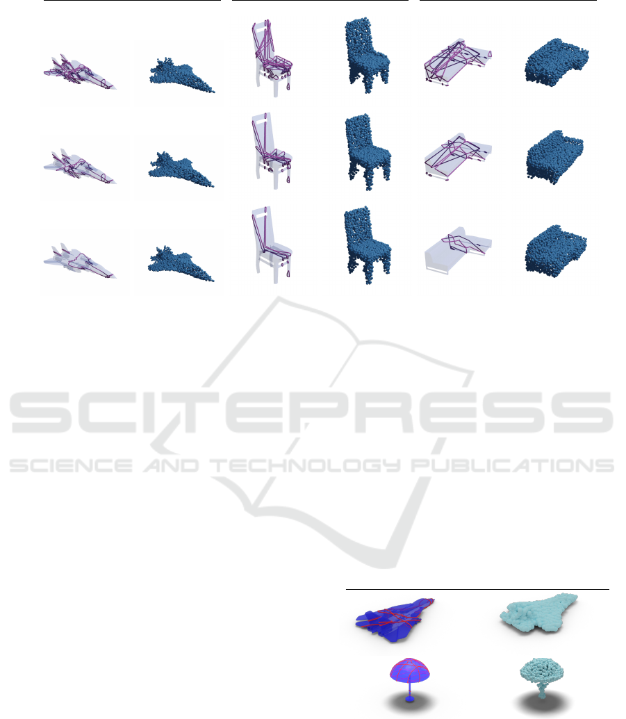
10 cross-sections5 cross-sections2 cross-sections
Figure 4: (Left) Comparison of reconstruction quality with an increasing number of cross-sections. Input to the network is
the set of cross-sections (red) belonging to the ground truth mesh (blue).
pair {G, D} we pass a ground truth point cloud P
gt
containing 2048 points through the encoder to gener-
ate an embedding, En(P
gt
). For a set of input parame-
terized cross-sections C, we create the piece-wise ad-
jacency matrix A
p
for each cross-section and a cross-
section adjacency matrix A
c
.
The generator is trained to generate an embedding
using the cross-section set C and the two adjacency
matrices for the point cloud. The generator loss is
given by
L
G
=log(1 − D (G (C, A
p
, A
c
),C, A
p
, A
c
))+
L
ch
(De(G(C, A
p
, A
c
)), De(En (P
gt
)))+
L
mse
(G(C, A
p
, A
c
), En (P
gt
)),
where L
ch
is the Chamfer loss between the point
clouds generated using the embedding estimated by
the generator and the embedding of the ground truth
point cloud. L
mse
is the mean squared error between
the embedding estimated by the generator and the em-
bedding of the ground truth point cloud. The discrim-
inator loss can be formulated as
L
D
=(1 − log (D (G (C, A
p
, A
c
),C, A
p
, A
c
)))+
log(D(En (P
gt
),C, A
p
, A
c
)),
where the discriminator is conditioned on the input
cross-section graph. The generator and discriminator
are trained in an adversarial manner (see (Goodfellow
et al., 2020)).
4 RESULTS AND DISCUSSION
We evaluate our approach on different classes of the
ShapeNet dataset. We perform an experimental pro-
cedure similar to DeepSDF where we divide the mod-
els into known shapes, i.e. shapes that were in the
training set and testing set referred to as unknown
shapes. We test our method in both single-class and
multi-class settings.
We show some samples for single-class training as
well in Figure 5. However, our key focus is on multi-
class training and its analysis is covered further.
Ground Truth with GCN output
cross-sections
Aircraft
Lamp
Figure 5: Results of the proposed model trained only on a
single class of objects. Input to the network are the cross-
sections (red) belonging to the ground truth mesh (blue).
We perform the training in a multi-class setting.
For the multiclass setting, we test on 4 classes - air-
plane (4K models), chair (6K models), lamp (2K
models), and sofa (3K models). Our implementation
GRAPP 2025 - 20th International Conference on Computer Graphics Theory and Applications
144

Table 1: Per-class Chamfer distance corresponding to varia-
tion in the number of cross-sections. Results for both under-
sampled and oversampled (> 10) cross-sections are shown
for a model trained on all aforementioned classes.
# cross- Per-class Chamfer distance Mean
sections Airplane Chair Lamp Sofa
2 0.4050 0.1765 2.7306 0.3770 0.9223
5 0.0493 0.0872 0.2394 0.0772 0.1133
10 0.0395 0.0829 0.0958 0.0728 0.0728
11 0.0385 0.0824 0.0927 0.0724 0.0715
15 0.0378 0.0813 0.0909 0.0715 0.0704
20 0.0374 0.0807 0.0898 0.0709 0.0697
25 0.0370 0.0803 0.0896 0.0704 0.0693
source code has been made available on Github. We
do not perform any class balancing techniques and
directly train on the ShapeNet dataset. We use py-
torch geometric (Fey and Lenssen, 2019) for this. We
demonstrate the impact of these attentions via an ab-
lative study in Table 2. We test inference time on
NVIDIA GTX 1070. The model takes ∼0.19 sec. for
generating point clouds from 10 cross-sections.
4.1 Cross-Section Dependence
We compare the mean Chamfer loss obtained across
the different classes for different numbers of input
cross-sections (5, 10, 11, 15, 20, and 25) provided
as input in Table 1. We observe results for the Cham-
fer distance obtained after training are shown in Table
1. We observe that the number of cross-sections pro-
vided as input has a vital control on the output of the
generated point cloud surface, as can be seen from
Table 1. We show the results of the proposed model
trained on four classes: Airplane, Chair, Lamp, and
Sofa with a different number of input parameterized
cross-sections in Figure 4. The even column displays
the ground truth mesh used to sample the ground truth
point cloud with cross-sections, and the odd column
shows the reconstruction with our method.
We discuss these trends and perform the t-SNE of
the embeddings and demonstrate how the distinguish-
ing capabilities of the network improve further with
increasing the number of cross-sections. Further, in
Figure 4, we show that despite the sharp reduction
in the number of cross-sections, the network still gen-
erates a reliable general shape for the class and can
distinguish between the classes of parametric forms.
4.2 Impact of Adjacency
We show the impact of different kinds of attention
mechanisms and study the empirical changes in Ta-
ble 2. Firstly, we use ring adjacency strictly for the
nodes, and secondly, we change the adjacency at the
higher levels. This is done with the intuition that the
network should be able to view all the nodes during
attention operation since nodes that are similar would
share similar embeddings at higher levels given that
they share similar local neighborhoods. Thirdly, we
provide a complete graph adjacency throughout all
the levels and allow the network to deduce the re-
lationships itself. In Table 2 summarizes the results
for different connectivity information that is fed to the
network. We observe that despite providing the exact
neighbor information in the form of ring adjacency,
the network performs best for a complete graph adja-
cency; we suspect that this is due to better information
capture since each neighbor of a node is no longer re-
stricted to the adjacent nodes in the cross-section but
can also accumulate information from nodes that are
not directly linked allowing the network to get a better
information gain thus reducing the impact of informa-
tion bottleneck that graph neural networks suffer from
as the depth of network increases.
Table 2: Impact of different Adjacency-based attentions.
Approach Chamfer Loss (mean)
Change in loss with different attention strategies
Attention Cross-section level only 0.33693247
Attention Piece level only 1.10052492
Without Attention 9.02284977
Change in loss with different connectivity
Complete Graph from first layer 0.86106642
Complete Graph at attention layers 5.80743287
Maintaining Ring Adjacency 9.57172529
4.3 Comparisons
This is a non-trivial task for many reconstruction
methods, as they often struggle to generate missing
structures from limited cross-sectional information.
Consequently, our approach holds practical value, as
it excels in accurately capturing the shape of objects
in scenarios where cross-section data is sparse.
We compare our method against 4 methods:
VIPSS (Huang et al., 2019) method for variational
surface reconstruction from cross-sections, surface
reconstruction from non-parallel curve networks (Liu
et al., 2008), a state of the art deep learning based
method P2P-Net (Yin et al., 2018) and the recent
OReX (Sawdayee et al., 2022) and show results in
Figure 6. Most of these methods suffer from holes
and instabilities for sparse cross-sections; therefore,
to be fair, we sample more cross-sections in those
cases. However, we restrict our method to 10 cross-
sections. VIPSS, OReX, and Liu’s method require
careful sampling and sometimes tend to fail randomly
for sparse cross-sections. We show the best-case re-
sults for these methods. VIPSS is very sensitive to λ
Curvy: A Parametric Cross-Section Based Surface Reconstruction
145
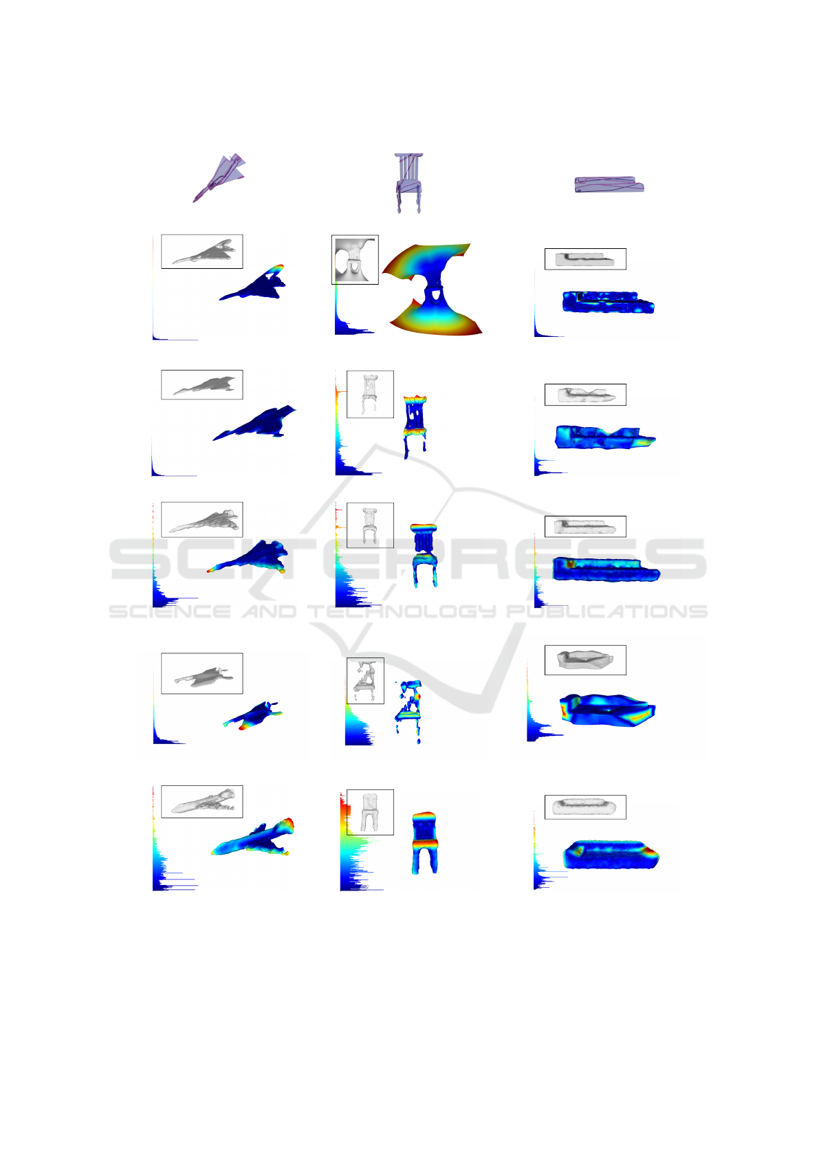
GT Mesh + Input
VIPSS (Huang et al., 2019)
d
H
: 0.032574 d
H
: 0.056161 d
H
: 0.001533
Liu et. al (Liu et al., 2008)
d
H
: 0.005765 d
H
: 0.039835 d
H
: 0.010035
P2P Net (Yin et al., 2018)
d
H
: 0.023185 d
H
: 0.032854 d
H
: 0.012473
OReX (Sawdayee et al., 2022)
d
H
: 0.022027 d
H
: 0.049031 d
H
: 0.015033
Ours
d
H
: 0.032111 d
H
: 0.049031 d
H
: 0.019826
Figure 6: Comparison with the state-of-the-art methods. The inset shows point-wise surface error compared with the GT. The
blue regions indicate areas of low error while brighter areas indicate higher error.
and requires a large number ∼ 80 of cross-sections for
faithful reconstruction due to failure due to openness
in cross-sections; however, we still notice artifacts.
We checked the reconstruction with the method
GRAPP 2025 - 20th International Conference on Computer Graphics Theory and Applications
146
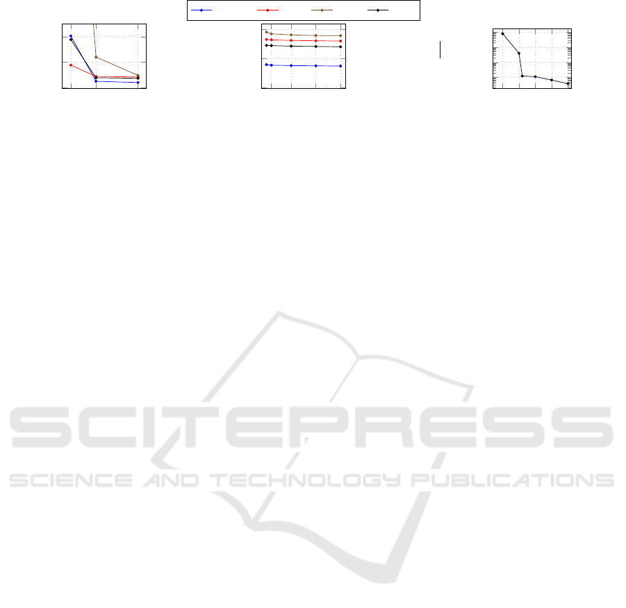
2
5
10
0
0.2
0.4
Number of cross-sections
L
ch
11
15
20
25
0
0.05
0.1
Number of cross-sections
L
ch
Aircraft Chair
Lamp
Sofa
2
5
10
15
20
25
10
−3
10
−2
10
−1
10
0
Number of cross-sections
−∆L
ch
(a) (b) (c)
Figure 7: Dependence of Chamfer loss L
ch
on the number of cross-sections. (a) Undersampling conditions, (b) Oversampling
conditions, (c) Negative change in mean Chamfer loss (log-scale).
proposed in (Liu et al., 2008), however, the avail-
able implementation discards many cross-sections
that lead to incorrect results. We show results for
the cases where we did not observe this issue for a
fair comparison. For OReX (Sawdayee et al., 2022)
as well, we observe that it performs really well when
cross-sections are dense; however, it fails in the case
of sparse cross-sections. Therefore, for some sam-
ples, we show results in cases where it performs rea-
sonably well.
We further compare our method against a state-of-
the-art deep learning-based method called P2P-Net.
We modify P2P Net and train it on points sampled
from our cross-sections. We notice that in some cases,
despite performing better in terms of metrics, there
are still completion issues in several samples, such as
the chair shown in Figure 6. Our method generates
symmetric structures leading to higher loss value but
better perception quality and semantically correct dif-
ferent structures such as the right-hand rest of the sofa
and missing leg in the chair. This also highlights a
weakness of our method pertaining to the lack of strict
adherence to the cross-sections since our method re-
lies on embedding decoded by the pre-trained de-
coder. However, we believe that can be circumvented
by better pre-training schemes since the performance
of the pre-trained decoder forms the lower bound of
the reconstruction error and can be swapped with any
of the better-performing point cloud generators.
In order to visualize the error in reconstruction
from our method and P2P-Net, we perform surface
meshing of our resulting point cloud with Poisson Re-
construction (Kazhdan et al., 2006) , by computing
normals from the ground truth mesh for the best-case
scenario. For VIPSS, we also modified the method
and provided normals from the GT mesh. We show
similar histograms for the surfaces obtained from
other methods. We also note the Hausdorff distance
(d
H
) obtained for different methods in Figure 6. We
notice that during the generation of the point cloud
since our method does not have hard constraints for
precise overlap with input, the shift in point cloud can
lead to a relative rise in the Hausdorff distance, as can
be seen in the case of the chair in Figure 6. However,
it outperforms the other methods in both qualitative
and quantitative comparisons in several cases.
4.4 Changes in Embedding
Since the graph embedding also varies as the num-
ber of cross-sections changes, we try to reason how
the class information of embedding varies as we in-
crease the number of cross-sections. In order to do
so, we compute the t-SNE (Van der Maaten and Hin-
ton, 2008) from the embedding vectors of 200 sam-
ples of each class in the multi-class setting and plot
them to see how the cluster distance varies with cross-
sections. From Figure 8 we observe that in the under-
sampling conditions the overlap between the clusters
increases, thus making it difficult for the network to
implicitly predict the class of the object, whereas as
the number of cross-sections is increased, the overlap
of clusters reduces. However, we also note that some
shapes exhibit a well-separated cluster even when the
number of cross-sections is less such as airplane in
this case. We also note that classes chair (denoted by
green) and sofa (denoted by grey), since these classes
are similar in shape, show weaker disentanglement in
the embedding space of cross-sections.
4.5 Loss Trends
In Figure 7(a) we see the case for undersampling,
as expected we observe that as the number of cross-
sections are reduced the amount of information sup-
plied to the network reduces, and hence the recon-
struction quality degrades. We also note that there is
a sharp dip in Chamfer loss when the cross-sections
are increased to 5, which is the minimum number
of cross-sections on which the network is trained.
Increasing the number of cross-sections to 10 im-
proves the reconstruction quality visually; however,
the changes in empirical values are not particularly
significant, with most variations occurring on the or-
Curvy: A Parametric Cross-Section Based Surface Reconstruction
147
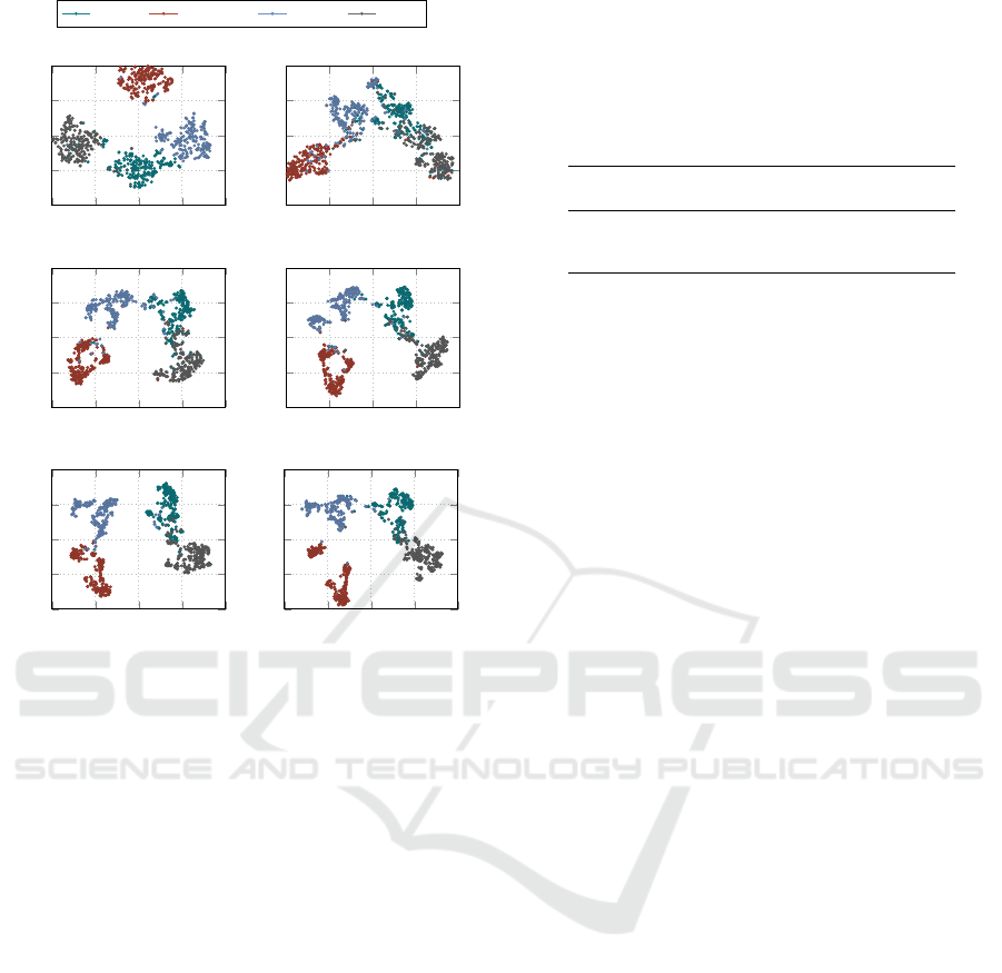
Chair Airplane
Lamp
Sofa
−40 −20 0 20 40
−40
−20
0
20
40
GT Embedding t-SNE
−40 −20 0 20 40
−40
−20
0
20
40
2 cross-sections
−40 −20 0 20 40
−40
−20
0
20
40
5 cross-sections
−40 −20 0 20 40
−40
−20
0
20
40
8 cross-sections
−40 −20 0 20 40
−40
−20
0
20
40
10 cross-sections
−40 −20 0 20 40
−40
−20
0
20
40
20 cross-sections
Figure 8: Changes in the t-SNE embedding clusters with
respect to the number of cross-sections.
der of 1e-3. This is evident in Figure 7(c), which de-
picts the case for oversampling when the number of
cross-sections is increased in the range of 15–25. In
the oversampling scenario, as shown in Figure 7(b),
a pronounced decline in the Chamfer distance is ob-
served up to 15 cross-sections. Beyond this point, fur-
ther increases in the number of cross-sections result in
minimal changes to the Chamfer distance. Nonethe-
less, the Chamfer distance continues to decrease grad-
ually as more information is provided to the network.
4.6 Variance in Loss
Further in Table 3, we show the standard deviations
for the losses across 20 different objects for vary-
ing cross-sections. We sample n ∈ {2, 5, 10} cross-
sections, randomly from the 100 cross-sections gen-
erated from the mesh as in our original experiment
setup and repeat this 40 times thus obtaining 40 ran-
dom samples for each object for a given n. We do this
to measure the standard deviation for the losses com-
puted for varying sampling of cross-sections. We first
compute the standard deviation obtained across dif-
ferent samples for the same object for a given value of
n. Then we compute the mean over the standard devi-
ations obtained across different objects for the given
n. This helps us to understand further the variations
for loss across cross-sections for each object.
Table 3: In the above table we demonstrate a similar trend of
reducing standard deviation in the chamfer losses obtained
for varying cross-sections for 20 different objects sampled
40 times each.
No. Airplane Lamp Sofa Chair
of cross-sections
2 0.09262 0.6465 0.0634 0.1131
5 0.01925 0.1060 0.0165 0.0243
10 0.00675 0.0253 0.0105 0.00985
We observe in Table 3 that similar to the reduction
in mean Chamfer Losses in Table 1 in the paper, the
standard deviations vary across classes and across the
number of cross-sections. If the mean for a particular
class is low so is the variance in the loss since the
model is able to faithfully reconstruct the shape given
any given set of cross-sections. Further, as the cross-
sections increase the amount of information provided
to the network increases thus the standard deviations
reduce across the same object sampled multiple times.
4.7 Failure Cases
This is a non-trivial task for many reconstruction
methods, as they often struggle to generate missing
structures from limited cross-sectional information.
In some cases, the failure of reconstruction is much
higher depending on the number of samples of a par-
ticular shape of the object the network sees and the
information in the cross-sections supplied. For ex-
ample, in Figure 10, in an airplane object, the cross-
sections do not contain sufficient information, leading
to a completely different object being created, though
it must be noted that the class of the reconstructed ob-
ject reconstructed is correct. We observe that in the
case of a failure, the network reconstructs a coarse
object of the correct class.
Further, we also notice a deterioration in the sam-
ples containing holes, such as chairs and lamps. For
example, in the case of the chair, the reconstruction
does not accurately maintain the genus of the object
for some samples.
5 CONCLUSION AND FUTURE
SCOPE
With this work, we open a new direction for the ex-
citing domain of cross-section-based reconstruction.
We generate a new dataset that can be used for multi-
ple tasks. The ability to use parametric cross-sections
directly in a learning-based setting exempts the use
GRAPP 2025 - 20th International Conference on Computer Graphics Theory and Applications
148
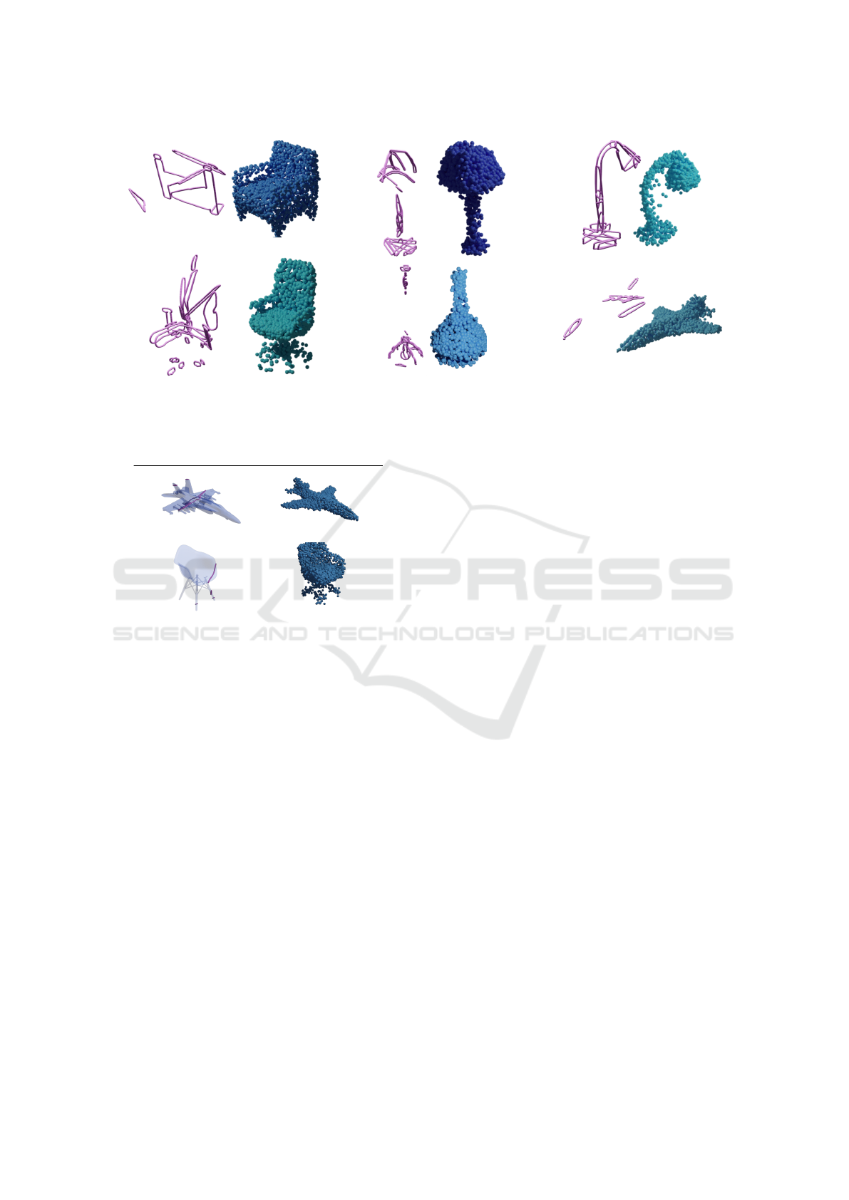
Figure 9: In above figure who show additional results consisting of the cross-sections (pink) and the corresponding point
clouds generated.
Ground Truth Predicted
Figure 10: Failure cases resulting in incorrect shapes. Input
to the network are cross-sections (red) belonging to the GT
mesh (white).
of any sampling-based restrictions in deep learning-
based methods. The complete information of the
curve is encapsulated in the coefficients of the para-
metric representation. Further, we utilize GCNs at
scale and demonstrate their effectiveness for para-
metric curves and the ability of the GCNs to capture
neighborhood information, which helps deduce bet-
ter relationships among the cross-sections using atten-
tion, adding to the explainability with the flexibility to
use any models trained on point cloud generation. We
show empirical evidence to analyze the changes in re-
construction, both in terms of the embedding space
representation and point cloud reconstruction, to un-
derstand the changes with respect to the variation in
the amount of information provided to the network.
This builds a strong motivation and opens up the field
to further research such as the disentanglement of la-
tent features and information-theoretic and in-depth
analysis of the cross-sections themselves which we
hope to cover in future works.
REFERENCES
Achlioptas, P., Diamanti, O., Mitliagkas, I., and Guibas, L.
(2018). Learning representations and generative mod-
els for 3D point clouds. In International conference
on machine learning, pages 40–49. PMLR.
Atzmon, M. and Lipman, Y. (2020). Sal: Sign agnostic
learning of shapes from raw data. In Proceedings of
the IEEE/CVF Conference on Computer Vision and
Pattern Recognition, pages 2565–2574.
Bajaj, C. L., Coyle, E. J., and Lin, K.-N. (1996). Arbi-
trary topology shape reconstruction from planar cross
sections. Graphical models and image processing,
58(6):524–543.
Boissonnat, J.-D. and Memari, P. (2007). Shape reconstruc-
tion from unorganized cross-sections. In Symposium
on geometry processing, pages 89–98. Citeseer.
Boyd, S. and Vandenberghe, L. (2018). Introduction to
applied linear algebra: vectors, matrices, and least
squares. Cambridge university press.
Brüel-Gabrielsson, R., Ganapathi-Subramanian, V., Skraba,
P., and Guibas, L. J. (2020). Topology-aware surface
reconstruction for point clouds. In Computer Graph-
ics Forum, volume 39, pages 197–207. Wiley Online
Library.
Chang, A. X., Funkhouser, T., Guibas, L., Hanrahan,
P., Huang, Q., Li, Z., Savarese, S., Savva, M.,
Song, S., Su, H., et al. (2015). ShapeNet: An
information-rich 3D model repository. arXiv preprint
arXiv:1512.03012.
Douglas, D. H. and Peucker, T. K. (1973). Algorithms for
the reduction of the number of points required to rep-
resent a digitized line or its caricature. Cartographica:
the international journal for geographic information
and geovisualization, 10(2):112–122.
Fan, H., Su, H., and Guibas, L. J. (2017). A point set gener-
ation network for 3D object reconstruction from a sin-
gle image. In Proceedings of the IEEE conference on
Curvy: A Parametric Cross-Section Based Surface Reconstruction
149

computer vision and pattern recognition, pages 605–
613.
Fey, M. and Lenssen, J. E. (2019). Fast graph represen-
tation learning with PyTorch Geometric. In ICLR
Workshop on Representation Learning on Graphs and
Manifolds.
Floater, M. S. and Surazhsky, T. (2006). Parameterization
for curve interpolation. In Studies in Computational
Mathematics, volume 12, pages 39–54. Elsevier.
Gadelha, M., Wang, R., and Maji, S. (2018). Multireso-
lution tree networks for 3D point cloud processing.
In Proceedings of the European Conference on Com-
puter Vision (ECCV), pages 103–118.
Goodfellow, I., Pouget-Abadie, J., Mirza, M., Xu, B.,
Warde-Farley, D., Ozair, S., Courville, A., and Ben-
gio, Y. (2020). Generative adversarial networks. Com-
munications of the ACM, 63(11):139–144.
Hamilton, W. L., Ying, R., and Leskovec, J. (2017). In-
ductive representation learning on large graphs. In
Proceedings of the 31st International Conference on
Neural Information Processing Systems, pages 1025–
1035.
Han, Z., Wang, X., Liu, Y.-S., and Zwicker, M. (2019).
Multi-angle point cloud-VAE: Unsupervised feature
learning for 3D point clouds from multiple angles by
joint self-reconstruction and half-to-half prediction. In
2019 IEEE/CVF International Conference on Com-
puter Vision (ICCV), pages 10441–10450. IEEE.
Huang, J. and Menq, C. (2002). Combinatorial manifold
mesh reconstruction and optimization from unorga-
nized points with arbitrary topology. Computer-Aided
Design, 34(2):149–165.
Huang, Z., Carr, N., and Ju, T. (2019). Variational implicit
point set surfaces. ACM Transactions on Graphics
(TOG), 38(4):1–13.
Huang, Z., Zou, M., Carr, N., and Ju, T. (2017). Topology-
controlled reconstruction of multi-labelled domains
from cross-sections. ACM Transactions on Graphics
(TOG), 36(4):1–12.
Kazhdan, M., Bolitho, M., and Hoppe, H. (2006). Poisson
surface reconstruction. In Eurographics.
Kipf, T. N. and Welling, M. (2017). Semi-supervised classi-
fication with graph convolutional networks. In 5th In-
ternational Conference on Learning Representations,
ICLR 2017.
Kuhn, H. W. and Tucker, A. W. (2014). Nonlinear program-
ming. In Traces and emergence of nonlinear program-
ming, pages 247–258. Springer.
Lazar, R., Dym, N., Kushinsky, Y., Huang, Z., Ju, T., and
Lipman, Y. (2018). Robust optimization for topo-
logical surface reconstruction. ACM Transactions on
Graphics (TOG), 37(4):1–10.
Lin, C.-H., Kong, C., and Lucey, S. (2018). Learning ef-
ficient point cloud generation for dense 3D object re-
construction. In proceedings of the AAAI Conference
on Artificial Intelligence, volume 32.
Liu, L., Bajaj, C., Deasy, J. O., Low, D. A., and Ju,
T. (2008). Surface reconstruction from non-parallel
curve networks. In Computer Graphics Forum, vol-
ume 27, pages 155–163. Wiley Online Library.
Memari, P. and Boissonnat, J.-D. (2008). Provably good 2D
shape reconstruction from unorganized cross-sections.
In Computer Graphics Forum, volume 27, pages
1403–1410. Wiley Online Library.
Park, J. J., Florence, P., Straub, J., Newcombe, R., and
Lovegrove, S. (2019). DeepSDF: Learning continuous
signed distance functions for shape representation. In
The IEEE Conference on Computer Vision and Pattern
Recognition (CVPR).
Peng, S., Jiang, C., Liao, Y., Niemeyer, M., Pollefeys, M.,
and Geiger, A. (2021). Shape as points: A differen-
tiable poisson solver. Advances in Neural Information
Processing Systems, 34:13032–13044.
Sarmad, M., Lee, H. J., and Kim, Y. M. (2019). RL-GAN-
Net: A reinforcement learning agent controlled gan
network for real-time point cloud shape completion.
In Proceedings of the IEEE/CVF Conference on Com-
puter Vision and Pattern Recognition, pages 5898–
5907.
Sawdayee, H., Vaxman, A., and Bermano, A. H.
(2022). Orex: Object reconstruction from planner
cross-sections using neural fields. arXiv preprint
arXiv:2211.12886.
Sharma, O. and Agarwal, N. (2017). Signed distance based
3D surface reconstruction from unorganized planar
cross-sections. Computers & Graphics, 62:67–76.
Van der Maaten, L. and Hinton, G. (2008). Visualizing data
using t-SNE. Journal of machine learning research,
9(11).
Vaswani, A., Shazeer, N., Parmar, N., Uszkoreit, J., Jones,
L., Gomez, A. N., Kaiser, Ł., and Polosukhin, I.
(2017). Attention is all you need. In Advances in
neural information processing systems, pages 5998–
6008.
Velickovic, P., Cucurull, G., Casanova, A., Romero, A., Liò,
P., and Bengio, Y. (2018). Graph attention networks.
In 6th International Conference on Learning Repre-
sentations, ICLR 2018.
Wen, X., Li, T., Han, Z., and Liu, Y.-S. (2020). Point cloud
completion by skip-attention network with hierarchi-
cal folding. In Proceedings of the IEEE/CVF Con-
ference on Computer Vision and Pattern Recognition,
pages 1939–1948.
Yin, K., Huang, H., Cohen-Or, D., and Zhang, H. (2018).
P2p-net: Bidirectional point displacement net for
shape transform. ACM Transactions on Graphics
(TOG), 37(4):1–13.
Zhou, K., Huang, X., Li, Y., Zha, D., Chen, R., and Hu, X.
(2020). Towards deeper graph neural networks with
differentiable group normalization. Advances in Neu-
ral Information Processing Systems, 33:4917–4928.
Zou, M., Holloway, M., Carr, N., and Ju, T. (2015).
Topology-constrained surface reconstruction from
cross-sections. ACM Transactions on Graphics
(TOG), 34(4):1–10.
GRAPP 2025 - 20th International Conference on Computer Graphics Theory and Applications
150
